Fractals/Iterations in the complex plane/def cqp

Definitions

Order is not only alphabetical but also by topic so use find (Ctrl-f)

See also

• Pictures_of_Julia_and_Mandelbrot_Sets - Terminology
• Index of Mu-Ency from Robert Munafo's home pages on HostMDS   © 1996-2020 Robert P. Munafo.

Address

 "Internal addresses encode kneading sequences in human-readable form, when extended to angled internal addresses they distinguish hyperbolic components in a concise and meaningful way. The algorithms are mostly based on Dierk Schleicher's paper Internal Addresses Of The Mandelbrot Set And Galois Groups Of Polynomials (version of February 5, 2008) http://arxiv.org/abs/math/9411238v2." Claude Heiland-Allen

• 

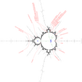
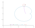
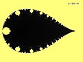
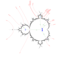  Parameter plane with internal rays (green) used for creating internal addresses

• 

  $1\xrightarrow {4/5} 5\xrightarrow {1/17} 85$

• 

  $1{\xrightarrow {1/3}}3{\xrightarrow {1/7}}21{\xrightarrow {1/13}}273$

• 

  $1\xrightarrow {1/3} 3\xrightarrow {1/3} 9$

• 

  $1\xrightarrow {1/2} 2\xrightarrow {1/3} 6$

types

• finite / infinite
• accesible/non-accesible
• on the parameter plane / on th edynamic plane
• simple/ angled
• for Crossed Renormalizations

Internal

• the internal address of a hyperbolic component A lists the periods of certain components that are “on the way” from the main cardioid to hyperbolic component A
• Internal addresses describe the combinatorial structure of the Mandelbrot set. It is one of the Analytical Naming Systems

 $1\quad {\xrightarrow {\quad }}\ 3\quad {\xrightarrow {\quad }}\ 6$

Internal address:

• is not constant within hyperbolic component. Example: internal address of -1 is 1->2 and internal address of 0.9999 is 1
• of hyperbolic component is defined as a internal address of it's center

angled

Angled internal address is an extension of internal address. The angled internal address of the end of a finite chain of child bulbs $p_{j}/q_{j},j\in 1,2,\ldots ,k$ would be:

$1\xrightarrow {p_{1}/q_{1}} q_{1}\xrightarrow {p_{2}/q_{2}} q_{1}q_{2}\ldots \xrightarrow {p_{k}/q_{k}} \prod _{j=1}^{k}q_{j}$

Examples:

• 

  $1\quad \xrightarrow {4/5} \ 5\quad \xrightarrow {1/17} \ 85\quad$

• $1\quad \xrightarrow {1/3} \ 3\quad \xrightarrow {1/2} \ 6\quad$ describes period 6 component which is a satelite of period 3 component.
• Mandelbrot Artists by Claude Heiland-Allen

Elements

• period of hyperbolic componnet
• angle of internal ray

One can see the adress as:

• sequence of hyperbolic components
• path inside Mandelbrot set

Path inside Mandelbrot set:

• start with center of period 1 ( nucleus)
• internal ray with angle n/m
• root point n/m ( bond)
• internal angle
• center with given period
• ...

Problems

Infinite sequences:

• islands
• infinite sequence of bifurcations

Angle

Types of angle

Principal branch or complex number argument

	external angle	internal angle	plain angle
parameter plane	$arg(\Phi _{M}(c))\,$	$arg(\rho _{n}(c))\,$	$arg(c)\,$
dynamic plane	$arg(\Phi _{c}(z))\,$		$arg(z)\,$

where:

• $\rho _{n}(c)$ is a multiplier map
• $\Phi (c)\,$ is a Boettcher function

external

The external angle is a angle of

• point of set's exterior
• the boundary.

It is:

• the same on all points on the external ray. It is important for proving connectedness of the Mandelbrot set.
• a proper fraction
• an approximation of directional derivative

internal

The internal angle is an angle of point of component's interior

• it is a rational number and proper fraction measured in turns (see multiplier map)
• it is the same for all point on the internal ray
• in a contact point (root point) it agrees with the rotation number
• root point has internal angle 0 (inside child component)
• "The internal angles start at 0, at the cusp, and increase counterclockwise. " Robert Munafo

$\alpha ={\frac {p}{q}}\in \mathbb {Q}$

See also

• binary search for internal angle . From the Mandelbrot Set Glossary and Encyclopedia, by Robert Munafo, (c) 1987-2022.     Mu-ency index

plain

The plain angle is an angle of complex point = its argument

Units

• turns
• degrees
• radians

Number types

Angle (for example, external angle in turns) can be used in different number types

Examples:

the external arguments of the rays landing at z = −0.15255 + 1.03294i are:

$(\theta _{20}^{-},\theta _{20}^{+})=(0.{\overline {00110011001100110100}},0.{\overline {00110011001101000011}})$

where:

$\theta _{20}^{-}=0.{\overline {00110011001100110100}}_{2}=0.{\overline {20000095367522590181913549340772}}_{10}={\frac {209716}{1048575}}={\frac {209716}{2^{20}-1}}$

Bifurcation

• Numerical Bifurcation Analysis of Maps
  • MatCont

Coordinate

Coordinate:

• Fatou coordinate for every repelling and attracting petal (linearization of function near parabolic fixed point)
• Boettcher
• Koenigs

   "The coordinates are the current location, measured on the x-y-z axis. The gradient is a direction to move from our current location" Sadid Hasan

Curves

Types:

• topology:
  • closed versus open
  • simple versus not simple
• other properities:
  • invariant
  • critical

Description

• plane curve = it lies in a plane.
• closed = it starts and ends at the same place.
• simple = it never crosses itself.

closed

Closed curves are curves whose ends are joined. Closed curves do not have end points.

• Simple Closed Curve: A connected curve that does not cross itself and ends at the same point where it begins. It divides the plane into exactly two regions (Jordan curve theorem). Examples of simple closed curves are ellipse, circle and polygons.
• Complex Closed Curve (not simple = non-simple) It divides the plane into more than two regions. Example: Lemniscates.

"non-self-intersecting continuous closed curve in plane" = "image of a continuous injective function from the circle to the plane"

Circle

Unit circle

Unit circle $\partial D\,$ is a boundary of unit disk

$\partial D=\left\{w:abs(w)=1\right\}$

where coordinates of $w\,$ point of unit circle in exponential form are:

$w=e^{i*t}\,$

Critical curves

Diagrams of critical polynomials are called critical curves.

These curves create skeleton of bifurcation diagram. (the dark lines)

dendrit

• a locally connected branched curve
• "Complex 1-variable polynomials with connected Julia sets and only repelling periodic points are called dendritic."
• "a dendrite is a locally connected continuum that does not contain Jordan curves."
• "a locally connected continuum without subsets homeomorphic to a circle"
• connected with no interior

See also:

• Misiurewicz point on the parameter plane
• Dendrite Modeling: Modeling dendrites, including trees, lightning, river systems, and all manner of branching structures, has been frequently undertaken in computer graphics. We propose a new dendritic modeling framework using path planning as the basic operation
• Procedural Branching Texture

Escape lines

Escape line = boundary of escape time's level sets

"If the escape radius is equal to 2 the contour lines have a contact point (c= -2) and cannot be considered as equipotential lines"

geodesic

In geometry, a geodesic is a curve representing in some sense the shortest path (arc) between two points in a surface

Integral

• integral curve is a parameterized curve, whose tangent vectors agree with the vectors from this vector field. In physics, integral curves for an electric field or magnetic field are known as field lines.

Invariant

Types:

• topological
• shift invariants

examples:

• curve is invariant for the map f (evolution function) if images of every point from the curve stay on that curve
• curve is invariant for a system of ordinary differential equations

"Quasi-invariant curves are used in the study of hedgehog dynamics" RICARDO PEREZ-MARCO

Examples:

• field lines
  • external ray
  • internal ray

Isocurves

Isocurve = level curve = curve which consist of points which have the same value (level) of parameter / variable

Equipotential lines

Equipotential lines = Isocurves of complex potential

"If the escape radius is greater than 2 the contour lines are equipotential lines"

Examples

• desmos examples: isovalues by Fabrice

Jordan curve

Illustration of the Jordan curve theorem. The Jordan curve (drawn in black) divides the plane into an "inside" region (light blue) and an "outside" region (pink).

Jordan curve = a simple closed curve that divides the plane into an "interior" region bounded by the curve and an "exterior" region containing all of the nearby and far away exterior points

Lamination

Lamination of the unit disk is a closed collection of chords in the unit disc, which can intersect only in an endpoint of each on the boundary circle

It is a model of Mandelbrot or Julia set.

A lamination, L, is a union of leaves and the unit circle which satisfies:

• leaves do not cross (although they may share endpoints) and
• L is a closed set.

"The pattern of rays landing together can be described by a lamination of the disk. As θ is varied, the diameter defined by θ/2 and (θ +1)/2 is moving and disconnecting or reconnecting chords. " Wolf Jung

Leaf

Chords = leaves = arcs

A leaf on the unit disc is a path connecting two points on the unit circle.

"In Thurston’s fundamental preprint, the two characteristic rays and their common landing point are the “minor leaf” of a “lamination”"

Level curve

LCM = Level Curve Method = method for drawing level curves

Examples:

• equipotential line (the same potential)
• external ray (the same external angle)
• boundary of level set (see Level Set Method = LSM)

Open curve

Curve which is not closed. Examples: line, ray.

Path

• Path in geometr is a curve

Ray

Rays are:

• invariant curves
• dynamic or parameter
• external, internal or extended

Extended

"We prolong an external ray R θ supporting a Fatou component U (ω) up to its center ω through an internal ray and call the resulting set the extended ray E θ with argument θ." Alfredo Poirier

External ray

The closure of an external ray is called a closed ray. If ray lands, then the closure of the ray is the union of the external ray and its landing point.

  "A ray R is said to land or converge, if the accumulation set ${\bar {R}}-R$ is a singleton subset of J.  The conjecture that the Mandelbrot set is locally connected is equivalent to the continuous landing of all external rays."

where:

• ${\bar {R}}$ is a closure of $R$ = the bar is taken to mean the closure rather than the complex conjugate
• MLC = Mandelbrot Local connectivity Conjecture: M is locally connected
• singelton set is a set with exactly one element

 "If the MLC were proved true, the theorem of Caratheodory would give us an extension of the Riemann map $\Phi :D\to Int(M)$ to $S1$, giving a conformal equivalence of M with D. Given the fractal nature of M, this would be a very surprising result.

Internal ray

Definition:

• "The internal rays are the preimages of the radial segments under the coordinate with componenet center corresponding to 0." Alfredo Poirier
• The internal rays of U are the images of radial lines under the Riemann maps.

Internal rays are:

• dynamic (on dynamic plane, inside filled Julia set)
• |parameter (on parameter plane, inside Mandelbrot set) usuning multiplier map

dynamic

• 

  Dynamic internal (blue segment) and external (red ray) rays

For a parameter c with superattracting orbit: for every Fatou component ${\mathit {U}}$ of filled julia set $K_{c}$ there is:

• a unique periodic or pre-periodic point $z_{\mathit {U}}$ of the super-attracting orbit
• a Riemann map that maps:

component to unit disc:

$\varphi _{\mathit {U}}:{\mathit {U}}\to \mathbb {D}$

and point $z_{\mathit {U}}$ to the origin:

$\varphi _{\mathit {U}}(z_{\mathit {U}})=0$

The point $z_{\mathit {U}}$ is called the center of component ${\mathit {U}}$.

For any angle $\vartheta \in \mathbb {R} /\mathbb {Z}$ the pre-image of the radial segment of the unit disc

$\varphi _{\mathit {U}}^{-1}(r^{2\pi \vartheta }):r\in [0,1]$

is called an internal ray of component ${\mathit {U}}$ with well-defined landing point.

where:

• $\mathbb {R} /\mathbb {Z}$ is The quotient group R/Z

See also:

• Hubbard tree

intertwined

The internal rays are the curves that connects endpoints of external rays to the origin (the only pole) by winding in the specific way through the Julia set. Unlike the external rays the internal rays allways cross other internal rays, usually at multiple points, hence they are interwined

parameter

• 
• 

  Uniformization of the interior of Mandelbrot set components using multiplier map: internal rays, internal coordinate

• 

  Method of computing internal ray using explicit equation

• 

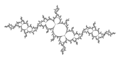
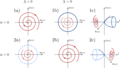
  Wakes near the period 3 island in the Mandelbrot set, internal angles and rays (green) and external angles and rays (red)

Escape route

Escape route is a path inside Mandelbrot set.

Escape route 1/2 <re>Plotting the Escape: An Animation of Parabolic Bifurcations in the Mandelbrot Set by Anne M. Burns. Mathematics Magazine Vol. 75, No. 2 (Apr., 2002), pp. 104-116 </ref>

• is part of the real slice of the mandelbrot set)
• part of the real line x=0

Steps:

• start from center of period 1
• go along internal ray 1/2 to root point of period 2 component
• go along internal ray 0 to the center of period 2 component
• go along internal ray 1/2 to root point of period 4 component
• ...

• escape routes
• 

  1/2

• 

  1/3

Spider

A spider S is a collection of disjoint simple curves called legs (extended rays = external + internal ray) in the complex plane connecting each of the post-critical points to infinity

See:

• spider algorithm
• spider program

Spine

• 

  Rabbit Julia set with spine

• 

  Basilica Julia set with spine

In the case of complex_quadratic_polynomial $f_{c}(z)=z^{2}+c$ the spine $S_{c}\,$ of the filled Julia set $\ K\,$ is defined as arc between $\beta \,$-fixed point and $-\beta \,$,

$S_{c}=\left[-\beta ,\beta \right]\,$

with such properties:

• spine lies inside $\ K\,$. This makes sense when $K\,$ is connected and full
• spine is invariant under 180 degree rotation,
• spine is a finite topological tree,
• Critical point $z_{cr}=0\,$ always belongs to the spine.
• $\beta \,$-fixed point is a landing point of external ray of angle zero ${\mathcal {R}}_{0}^{K}$,
• $-\beta \,$ is landing point of external ray ${\mathcal {R}}_{1/2}^{K}$.

Algorithms for constructing the spine:

• detailed version is described by A. Douady
• Simplified version of algorithm:
  • connect $-\beta \,$ and $\beta \,$ within $K\,$ by an arc,
  • when $K\,$ has empty interior then arc is unique,
  • otherwise take the shortest way that contains $0$.

Curve $R\,$:

$R\ {\overset {\underset {\mathrm {def} }{}}{=}}\ R_{1/2}\ \cup \ S_{c}\ \cup \ R_{0}\,$

divides dynamical plane into two components.

Computing external angle for c from centers of hyperbolic components and Misiurewicz points:

 The spine of K is the arc from beta to minus beta. Mark 0 each time C is above the spine and 1 each time it is below. You obtain the expansion in base 2 of the external argument theta of z by C. This simply comes from the two following facts:  
 *  0 < theta < 1/2 if acces to z is above the spine,   1/2 < theta < 1 if it is below
 * function f doubles the external arguments with respect to K, as well as the potential, since  Riemman map (Booettcher map) conjugates f to $z\to z^{2}$.
 Note that if c and z are real, the tree reduces to the segment [beta',beta] of the real line, and the sequence of 0 and 1 obtained is just the kneading sequence studied by Milnor and Thurston (except for convention: they use 1 and -1). 
 This sequence appears now as the binary expansion of a number which has a geometrical interpretation. " A. Douady

Relation between spine and major leaf of the lamination

Vein

"A vein in the Mandelbrot set is a continuous, injective arc inside in the Mandelbrot set"

"The principal vein $v_{p/q}$ is the vein joining $c_{p/q}$ to the main cardioid" (Entropy, dimension and combinatorial moduli for one-dimensional dynamical systems. A dissertation by Giulio Tiozzo)

Discriminant

In algebra, the discriminant of a polynomial is a polynomial function of its coefficients, which allows deducing some properties of the roots without computing them.

Distance

Distance Function

See also:

• metric
• Algorithm
  • Distance Estimation Method
    • DEM/J
    • DEM/M
  • SDF = Signed Distance Function
• distance fields
  • EDT Euclidean Distance Transform
  • SEDT = squared Euclidean distance transform. Algorithms generating distance fields from boolean fields:
    • Marching Parabolas, a linear-time CPU-amenable algorithm.
    • Min Erosion, a simple-to-implement GPU-amenable algorithm.

Dynamics

• symbolic
• complex
• Arithmetic
• combinatorial
• local/global
• discrete/continous
• parabolic/hyperbolic/eliptic

Examples:

• discrete local complex parabolic dynamics

evolution of dynamics along escape route 0 ( parabolic implosion); Im(c) = 0

parameter c	location of c	Julia set	interior	type of critical orbit dynamics	critical point	fixed points	stability of alfa
c = 0	center, interior	connected = Circle Julia set	exist	superattracting	attracted to alfa fixed point	fixed critical point equal to alfa fixed point, alfa is superattracting, beta is repelling	r = 0
0<c<1/4	internal ray 0, interior	connected	exist	attracting	attracted to alfa fixed point	alfa is attracting, beta is repelling	0 < r < 1.0
c = 1/4	cusp, boundary	connected = cauliflower	exist	parabolic	attracted to alfa fixed point	alfa fixed point equal to beta fixed point, both are parabolic	r = 1
c>1/4	external ray 0, exterior	disconnected = imploded cauliflower	disappears	repelling	repelling to infinity	both finite fixed points are repelling	r > 1

symbolic

"Symbolic dynamics encodes:

• a dynamical system $f:X\to X$ by a shift map on a space of sequences over finite alphabet using Markov partition of the space $X$
• the points of space $X$ by their itineraries with respect to the partition " (Volodymyr Nekrashevych - Symbolic dynamics and self-similar groups)

entropy

• image entropy

equation

differential

differential equations

• exact analytic solutions.
• approximated solution
  • use perturbation theory to approximate the solutions

Field

Field is a region in space where each and every point is associated with a value.

The field types according to the value type:

• scalar field
  • Distance field – Some mapping $R^{n}\to R$, where for any given input the output is the distance to the nearest surface (where the field value is 0).
• vector field, for example gradient field

Function

Derivative

• Derivative of Iterated function (map)
• of the function f with respect to (wrt) variable
• following the derivative

angular

Angular derivative

The Schwarzian Derivative

The Schwarzian Derivative

gradient

the gradient is the generalization of the derivative for the multivariable functions

definitions:

• (field): Gradient field is the vector field with gradient vector
• (function): The gradient of a scalar-valued multivariable function $f(x,y)$ is a vector-valued function denoted $\nabla f$
• (vector): The gradient of the function f at the point (x,y) is defined as the unique vector (result of gradient function) representing the maximum rate of increase of a scalar function (length of the vector) and the direction of this maximal rate (angle of the vector). Such vector is given by the partial derivatives with respect to each of the independent variables
• (operator): Del or nabla is an gradient operator = a vector differential operator

• 

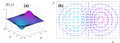  Gradient 2D field with gradient vectors

• 

  one gradient vector (red)

Notations:

$\nabla f(x,y)=[{\frac {\partial f}{\partial x}},{\frac {\partial f}{\partial y}}]={\begin{bmatrix}{\frac {\partial f}{\partial x}}\\{\frac {\partial f}{\partial y}}\end{bmatrix}}={\frac {\partial f}{\partial x}}\mathbf {i} +{\frac {\partial f}{\partial y}}\mathbf {j}$

$\operatorname {grad} f=\nabla f$

See also

• Gradient Descent Algorithm
• Gradient Ascent Algorithm
• image gradient

Jacobian

The Jacobian is the generalization of the gradient for vector-valued functions of several variables

multiplier

The multiplier of a fixed point α is the derivative A′(α) calculated in any local chart around α

Germ

Germ of the function f in the neighborhood of point z is a set of the functions g which are indistinguishable in that neighborhood

$[f]_{z}=\{g:g\sim _{z}f\}.$

See:

• parabolic germ
• the linearization of a germ

map

• differences between map and the function
• Iterated function = map
• an evolution function of the discrete nonlinear dynamical system

$z_{n+1}=f(z_{n})\,$

is called map $f$, examples:

• rational maps
  • Newton maps
  • complex quadratic map: $f_{c}:z\to z^{2}+c.\,$
• exponential maps
• trigonometric maps
• landing map: " A theorem of Caratheodory states that if $K\subset \mathbb {C}$ is a full compact and locally connected set, then external rays land and the landing map $\ell :\mathbb {R} /\mathbb {Z} \to \partial K$ is continuous."

types or names

Brjuno

• Brjuno function

Links:

• Quelle est la régularité de la fonction de Brjuno ?

harmonic

An harmonic or spherical function is a:

• "set of orthogonal functions all of whose curvatures are changing at the same rate."
• "harmonic functions relate two sets of different curves such that the rate of change of their respective curvatures is always equal. " and they are orthogonal
• "One set of curves of the harmonic function expressed the pathways of minimal change in the potential for action, while the other, orthogonal curves expressed the pathways of maximum change in the potential for action."
• "a pair of harmonic conjugate functions, u and v. They satisfy the Cauchy-Riemann equations. Geometrically, this implies that the contour lines of u and v intersect at right angles"

Geometric examples:

• " A set of concentric circles and radial lines comprises an harmonic function because both the circles and the radial lines intersect orthogonally and both have constant curvature."
• "a set of orthogonal ellipses and hyperbolas."

How to find harmonic conjugate function ?

meromorphic

meromorphic maps: Those with NO FINITE, NON-ATTRACTING FIXED POINTS

Polynomial

Critical

Critical polynomial:

$Q_{n}=f_{c}^{n}(z_{cr})=f_{c}^{n}(0)\,$

so

$Q_{1}=f_{c}^{1}(0)=c\,$

$Q_{2}=f_{c}^{2}(0)=c^{2}+c\,$

$Q_{3}=f_{c}^{3}(0)=(c^{2}+c)^{2}+c\,$

These polynomials are used for finding:

• centers of period n Mandelbrot set components. Centers are roots of n-th critical polynomials $centers=\{c:f_{c}^{n}(z_{cr})=0\}\,$ (points where critical curve Qn croses x axis)
• Misiurewicz points $M_{n,k}=\{c:f_{c}^{k}(z_{cr})=f_{c}^{k+n}(z_{cr})\}\,$

post-critically finite

a post-critically finite polynomial = all critical points have finite orbit

Resurgent

"resurgent functions display at each of their singular points a behaviour closely related to their behaviour at the origin. Loosely speaking, these functions resurrect, or surge up - in a slightly different guise, as it were - at their singularities"

J. Écalle, 1980

transformation

In mathematics, a transformation is a function f, usually with some geometrical underpinning, that maps a set X to itself, i.e. f : X → X.

Examples include:

• linear transformations of vector spaces
• geometric transformations
  • projective transformations
  • affine transformations
    • rotations
    • reflections
    • translations

coordinate transformations

There are often many different possible coordinate systems for describing geometrical figures. The relationship between different systems is described by coordinate transformations, which give formulas for the coordinates in one system in terms of the coordinates in another system. For example, in the plane, if Cartesian coordinates (x, y) and polar coordinates (r, θ) have the same origin, and the polar axis is the positive x axis, then the coordinate transformation from polar to Cartesian coordinates is given by x = r cosθ and y = r sinθ.

With every bijection from the space to itself two coordinate transformations can be associated:

• Such that the new coordinates of the image of each point are the same as the old coordinates of the original point (the formulas for the mapping are the inverse of those for the coordinate transformation)
• Such that the old coordinates of the image of each point are the same as the new coordinates of the original point (the formulas for the mapping are the same as those for the coordinate transformation)

For example, in 1D, if the mapping is a translation of 3 to the right, the first moves the origin from 0 to 3, so that the coordinate of each point becomes 3 less, while the second moves the origin from 0 to −3, so that the coordinate of each point becomes 3 more.

glitches

Interior of the Cauliflower Julia set. .The black structure around fixed point and it's preimages is a numerical error (glitch) }}

Definition:

• Incorrect (noisy) parts of renders using perturbation technique
• pixels which dynamics differ significantly from the dynamics of the reference pixel"These can be detected and corrected by using a more appropriate reference."

Examples:

• glitches in perturbation method

graf

Dessin d'enfant

• Wikipedia article: Dessin d'enfant
• commons:Category:Dessins d'enfants (mathematics)

See also:

• Polynomials Invertible in k-Radicals by Y. Burda, A. Khovanskii

Tree

• fractalforums.org: functional-graph-of-modular-arithmetic
• Oleg Ivrii (Tel Aviv University), "Shapes of trees"

Farey tree

Farey tree = Farey sequence as a tree

Hubbard tree

• a simplified, combinatorial model of the Julia set (MARY WILKERSON)
• "Hubbard trees are finite planar trees, equipped with self-maps, which classify postcritically finite polynomials as holomorphic dynamical systems on the complex plane."
• " Hubbard trees are invariant trees connecting the points of the critical orbits of post-critically finite polynomials. Douady and Hubbard showed in the Orsay Notes that they encode all combinatorial properties of the Julia sets. For quadratic polynomials, one can describe the dynamics as a subshift on two symbols, and itinerary of the critical value is called the kneading sequence." Henk Bruin and Dierk Schleicher

Rooted tree

rooted tree of preimages:

$T_{f}:=\bigsqcup _{n\geq 0}f^{-n}(t),$

where a vertex $z\in f^{-n}(t)$ is connected by an edge with $f(z)\in f^{-(n-1)}(t)$.

Iteration

Iteration

Magnitude

• magnitude of the point (complex number in 2D case) = it's distance from the origin
• radius is the absolute value of complex number (compare to arguments or angle)

Map

description

types

• The map f is hyperbolic if every critical orbit converges to a periodic orbit.

Complex quadratic map

Forms

c form: $z^{2}+c$

quadratic map

• math notation: $f_{c}(z)=z^{2}+c\,$
• Maxima CAS function:

f(z,c):=z*z+c;

(%i1) z:zx+zy*%i;
(%o1) %i*zy+zx
(%i2) c:cx+cy*%i;
(%o2) %i*cy+cx
(%i3) f:z^2+c;
(%o3) (%i*zy+zx)^2+%i*cy+cx
(%i4) realpart(f);
(%o4) -zy^2+zx^2+cx
(%i5) imagpart(f);
(%o5) 2*zx*zy+cy

Iterated quadratic map

• math notation

$\ f_{c}^{(0)}(z)=z=z_{0}$

$\ f_{c}^{(1)}(z)=f_{c}(z)=z_{1}$

...

$\ f_{c}^{(p)}(z)=f_{c}(f_{c}^{(p-1)}(z))$

or with subscripts:

$\ z_{p}=f_{c}^{(p)}(z_{0})$

• Maxima CAS function:

fn(p, z, c) :=
  if p=0 then z
  elseif p=1 then f(z,c)
  else f(fn(p-1, z, c),c);

zp:fn(p, z, c);

lambda form: $z^{2}+\lambda z$

More description Maxima CAS code (here m not lambda is used):

(%i2) z:zx+zy*%i;
(%o2) %i*zy+zx
(%i3) m:mx+my*%i;
(%o3) %i*my+mx
(%i4) f:m*z+z^2;
(%o4) (%i*zy+zx)^2+(%i*my+mx)*(%i*zy+zx)
(%i5) realpart(f);
(%o5) -zy^2-my*zy+zx^2+mx*zx
(%i6) imagpart(f);
(%o6) 2*zx*zy+mx*zy+my*zx

Switching between forms

Start from:

• internal angle $\theta ={\frac {p}{q}}$
• internal radius r

Multiplier of fixed point:

$\lambda =re^{2\pi \theta i}$

When one wants change from lambda to c:

$c=c(\lambda )={\frac {\lambda }{2}}\left(1-{\frac {\lambda }{2}}\right)={\frac {\lambda }{2}}-{\frac {\lambda ^{2}}{4}}$

or from c to lambda:

$\lambda =\lambda (c)=1\pm {\sqrt {1-4c}}$

Example values:

$\theta$	r	c	fixed point alfa $z_{c}$	$\lambda$	fixed point $z_{\lambda }$
1/1	1.0	0.25	0.5	1.0	0
1/2	1.0	-0.75	-0.5	-1.0	0
1/3	1.0	0.64951905283833*i-0.125	0.43301270189222*i-0.25	0.86602540378444*i-0.5	0
1/4	1.0	0.5*i+0.25	0.5*i	i	0
1/5	1.0	0.32858194507446*i+0.35676274578121	0.47552825814758*i+0.15450849718747	0.95105651629515*i+0.30901699437495	0
1/6	1.0	0.21650635094611*i+0.375	0.43301270189222*i+0.25	0.86602540378444*i+0.5	0
1/7	1.0	0.14718376318856*i+0.36737513441845	0.39091574123401*i+0.31174490092937	0.78183148246803*i+0.62348980185873	0
1/8	1.0	0.10355339059327*i+0.35355339059327	0.35355339059327*i+0.35355339059327	0.70710678118655*i+0.70710678118655	0
1/9	1.0	0.075191866590218*i+0.33961017714276	0.32139380484327*i+0.38302222155949	0.64278760968654*i+0.76604444311898	0
1/10	1.0	0.056128497072448*i+0.32725424859374	0.29389262614624*i+0.40450849718747	0.58778525229247*i+0.80901699437495

One can easily compute parameter c as a point c inside main cardioid of Mandelbrot set:

$c=c_{x}+c_{y}*i$

of period 1 hyperbolic component (main cardioid) for given internal angle (rotation number) t using this c / cpp code by Wolf Jung

 double InternalAngleInTurns;
 double InternalRadius;
 double t = InternalAngleInTurns *2*M_PI; // from turns to radians
 double R2 = InternalRadius * InternalRadius;
 double Cx, Cy; /* C = Cx+Cy*i */
 // main cardioid
 Cx = (cos(t)*InternalRadius)/2-(cos(2*t)*R2)/4; 
 Cy = (sin(t)*InternalRadius)/2-(sin(2*t)*R2)/4;

or this Maxima CAS code:

 
/* conformal map  from circle to cardioid (boundary
 of period 1 component of Mandelbrot set */
F(w):=w/2-w*w/4;

/* 
circle D={w:abs(w)=1 } where w=l(t,r) 
t is angle in turns ; 1 turn = 360 degree = 2*Pi radians 
r is a radius 
*/
ToCircle(t,r):=r*%e^(%i*t*2*%pi);

GiveC(angle,radius):=
(
 [w],
 /* point of  unit circle   w:l(internalAngle,internalRadius); */
 w:ToCircle(angle,radius),  /* point of circle */
 float(rectform(F(w)))    /* point on boundary of period 1 component of Mandelbrot set */
)$

compile(all)$

/* ---------- global constants & var ---------------------------*/
Numerator :1;
DenominatorMax :10;
InternalRadius:1;

/* --------- main -------------- */
for Denominator:1 thru DenominatorMax step 1 do
(
 InternalAngle: Numerator/Denominator,
 c: GiveC(InternalAngle,InternalRadius),
 display(Denominator),
 display(c),
  /* compute fixed point */
 alfa:float(rectform((1-sqrt(1-4*c))/2)), /* alfa fixed point */
 display(alfa)
 )$

Circle map

Circle map

• irrational rotation

Doubling map

Angle doubling map

$T(x)=(2x){\bmod {1}}$

Feigenbaum map

"the Feigenbaum map F is a solution of Cvitanovic-Feigenbaum equation"

First return map

• definition
• video: Intro to Poincare map (Poincaré), the first return map. This map helps us determine the stability of a limit cycle using the eigenvalues (Floquet multipliers) associated with the map.

"In contrast to a phase portrait, the return map is a discrete description of the underlying dynamics. .... A return map (plot) is generated by plotting one return value of the time series against the previous one "

"If x is a periodic point of period p for f and U is a neighborhood of x, the composition $f^{\circ p}\,$ maps U to another neighborhood V of x. This locally defined map is the return map for x." (W P Thurston: On the geometry and dynamics of Iterated rational maps)

"The first return map S → S is the map defined by sending each x0 ∈ S to the point of S where the orbit of x0 under the system first returns to S."

"way to obtain a discrete time system from a continuous time system, called the method of Poincar´e sections Poincar´e sections take us from: continuous time dynamical systems on (n + 1)-dimensional spaces to discrete time dynamical systems on n-dimensional spaces"

postcritically finite

postcritically finite: maps whose critical orbits are all periodic or preperiodic

  " In the theory of iterated rational maps, the easiest maps to understand are postcritically finite: maps whose critical orbits are all periodic or preperiodic. These maps are also the most important maps for understanding the combinatorial structure of parameter spaces of rational maps. "

A postcritically finite quadratic polynomial fc(z) = z^2+c may be:

• periodic of satellite type
• periodic of primitive type
• critically preperiodic (Misiurewicz type)

Examples are given by:

• the Basilica Q(z) = z^2 − 1
• the Kokopelli
• P(z) = z^2 + i (dendrite)

Critically preperiodic polynomials

• the critical point of fc is strictly preperiodic
• parameter c is from Thurston-Misiurewicz points–values on the boundary of the Mandelbrot set = Misiurewicz point
• Julia set is dendrite

Multiplier map

Mandelbrot set - multiplier map

Multiplier map $\lambda$ associated with hyperbolic component $\mathrm {H}$

• gives an explicit uniformization of hyperbolic component $\mathrm {H}$ by the unit disk $\mathbb {D}$:
• it is (d-1) to one function. Where d is a degree of iterated function

$\lambda _{p}:\mathrm {H} \to \mathbb {D}$

In other words it maps hyperbolic component H to unit disk D.

It maps point c from parameter plane to point b from reference plane:

$\lambda _{p}(c)=b$

where:

• c is a point in the parameter plane
• b is a point in the reference plane. It is also internal coordinate
• $\lambda$ is a multiplier map

Multiplier map is a conformal isomorphism.

It can be computed using:

• Newton method: internal_coordinate by Claude Heiland-Allen
• m-interior function
• First derivative wrt z

Approximation

• Mapping a polar grid onto the Mandelbrot Set on iteration at a time.by Maths town

Riemann map

Riemann mapping theorem says that every simply connected subset U of the complex number plane can be mapped to the open unit disk D

$f:U\to D$

where:

• D is a unit disk $D=\{z\in \mathbf {C} :|z|<1\}.$
• f is Riemann map (function). It is 1to-1 function
• U is subset of complex plane

• 

  Multiplier map

• 

  BDM

• 

  MBDM

• 

  DLD

• 

  SAC

Examples (approximations of Riemann mapping):

• multiplier map on the parameter plane
• binary decomposition
• Böttcher coordinates
  • on the parameter plane the Riemann map for the complement of the Mandelbrot set
  • on dynamic plane
    • for the Fatou component containing a superattracting fixed point for a rational map
    • a Riemann map for the complement of the filled Julia set of a quadratic polynomial with connected Julia: "The Riemann map for the central component for the Basilica was drawn in essentially the same way, except that instead of starting with points on a big circle, I started with sample points on a circle of small radius (e.g. 0.00001) around the origin." Jim Belk

function:

• explicit formula (only in simple cases)
• numerical approximation (in most of the cases)
  • Zipper
    • https://code.google.com/archive/p/zipper/
    • https://sites.math.washington.edu/~marshall/zipper.html
  • " Thurston and others have done some beautiful work involving approximating arbitrary Riemann maps using circle packings. See Circle Packing: A Mathematical Tale by Stephenson."
  • " To some extent, constructing a Riemann map is simply a matter of constructing a harmonic function on a given domain (as well as the associated harmonic conjugate), subject to certain boundary conditions. The solution to such problems is a huge topic of research in the study of PDE's, although the connection with Riemann maps is rarely mentioned." Jim Belk

PDE's approach to construct a Riemann map explicitly on a given domain D

• First, translate the domain so that it contains the origin.
• Next, use a numerical method to construct a harmonic function F satisfying

 $F(z)\;=\;-\log |z|$

for all $z\in \partial D$, and let

 $R(z)=|z|e^{F(z)}$

Then

• $R(0)=0$
• $R|_{\partial D}\equiv 1$
• and $\log R$ is harmonic

so:

• R is the radial component (i.e. modulus) of a Riemann map on D.
• The angular component can now be determined by the fact that its level curves are perpendicular to the level curves of R, and have equal angular spacing near the origin."

"Using the Riemann mapping BM we can define the parameter external rays and equipotentials as the preimages of the straight rays going to ∞ and round circles centered at 0. This gives us two orthogonal foliations in the complement of the Mandelbrot set." 

See

• Commons: Category:Riemann mapping
• A Riemann map on the central component
• Some internal rays of the Basilica
• The Bottcher Map B gives rise to internal angles in each bubble

Rotation map

     "If a is rational, then every point is periodic. If a is irrational, then every point has a dense orbit." David Richeson

rational

Rotation map $R$ describes counterclockwise rotation of point $\theta$ thru ${\frac {p}{q}}$ turns on the unit circle:

 $R_{\frac {p}{q}}(\theta )=\theta +{\frac {p}{q}}$

It is used for computing:

• itinerary

• rotation maps
• 
• 

irrational

• ROTATE IN A CIRCLE WITH A ROTATION by Sylvie Ruette (in fr.)
• Wikipedia: Irrational rotation

Shift map

names:

• bit shift map (because it shifts the bit) = if the value of an iterate is written in binary notation, the next iterate is obtained by shifting the binary point one bit to the right, and if the bit to the left of the new binary point is a "one", replacing it with a zero.
• 2x mod 1 map (because it is math description of its action)

Shift map (one-sided binary left shift) acts on one-sided infinite sequence of binary numbers by

 $\sigma (b_{1},b_{2},b_{3},\ldots )=(b_{2},b_{3},b_{4},\ldots )$

It just drops first digit of the sequence.

  $\sigma ^{2}(S)=\sigma (\sigma (S))$

  $\sigma ^{k}(b_{1}b_{2}\ldots )=b_{k+1}b_{k+2}\ldots$

If we treat sequence as a binary fraction:

 $x=0.b_{1},b_{2},b_{3},\ldots$

then shift map = the dyadic transformation = dyadic map = bit shift map= 2x  mod 1 map = Bernoulli map = doubling map = sawtooth map

 $\sigma (x)=2x{\bmod {1}}$

and "shifting N places left is the same as multiplying by 2 to the power N (written as 2N)" (operator <<)

In Haskell:

 shift k = genericTake q . genericDrop k . cycle  -- shift map

See also:

• How to compute external angles of principal Misiurewicz points of wakes?
• On quotients of the shift associated with dendrite Julia sets of quadratic polynomials by Christopher Penrose Published 1990

Number

complex number

• numerical value: x+y*i
• vector from origin to point (x,y)
• point (x,y) od 2D Cartesion plain

constant

Fegenbaum constant

• first (delta)
• second (alpha)

How to compute:

• Keith Briggs: How to calculate
• octave program by Anton Hendricson
• python program by cdlane
• Rosettacode
• An efficient method for the computation of the Feigenbaum constants to high precision by Andrea Molteni (Submitted on 7 Feb 2016)

degree

It hase many meanings:

• unit of the angle
• degree of a function
  • polynomial
  • rational function

Multiplier

The multiplier of periodic z-point:

• is a complex number
• "The value of $(f^{p})^{\prime }$ is the same at any point in the orbit of a: it is called the multiplier of the cycle."
• The multiplier is invariant under conjugacy
• Linearizability depends on the multiplier

Math notation:

$\lambda _{c}(z)={\frac {df_{c}^{(p)}(z)}{dz}}\,$

Maxima CAS function for computing multiplier of periodic cycle:

m(p):=diff(fn(p,z,c),z,1);

where p is a period. It takes period as an input, not z point.

period	$f^{p}(z)\,$	$\lambda _{c}(z)\,$
1	$z^{2}+c\,$	$2z\,$
2	$z^{4}+2cz^{2}+c^{2}+c$	$4z^{3}+4cz$
3	$z^{8}+4cz^{6}+6c^{2}z^{4}+2cz^{4}+4c^{3}z^{2}+4c^{2}z^{2}+c^{4}+2c^{3}+c^{2}+c$	$8z^{7}+24cz^{5}+24c^{2}z^{3}+8cz^{3}+8c^{3}z+8c^{2}z$

It is used to:

• compute stability index of periodic orbit (periodic point) = $|\lambda |=r$ (where r is a n internal radius)
• multiplier map

"The multiplier of a fixed point gives information about its stability (the behaviour of nearby orbits)"

See also:

• multiplier map
• Buff, Xavier. “VIRTUALLY REPELLING FIXED POINTS.” Publicacions Matemàtiques, vol. 47, no. 1, Universitat Autònoma de Barcelona, 2003, pp. 195–209, http://www.jstor.org/stable/43736773.

Rotation number

The rotation number of the disk (component) attached to the main cardioid of the Mandelbrot set is a proper, positive rational number p/q in lowest terms where:

• q is a period of attached disk (child period) = the period of the attractive cycles of the Julia sets in the attached disk
• p describes fc action on the cycle: fc turns clockwise around z0 jumping, in each iteration, p points of the cycle

Features:

• in a contact point (root point) it agrees with the internal angle
• the rotation numbers are ordered clockwise along the boundary of the componant
• " For parameters c in the p/q-limb, the filled Julia set Kc has q components at the fixed point αc . These are permuted cyclically by the quadratic polynomial fc(z), going p steps counterclockwise " Wolf Jung

Winding number

• of the map (iterated function)
  • "the winding number of the dynamic ray at angle a around the critical value, which is defined as follows: denoting the point on the dynamic a-ray at potential t greater or equal to zero by zt and decreasing t from +infinity to 0, the winding number is the total change of arg(zt - c) (divided by 2*Pi so as to count in full turns). Provided that the critical value is not on the dynamic ray or at its landing point, the winding number is well-defined and finite and depends continuously on the parameter. " DIERK SCHLEICHER
  • "the winding number of the dynamic ray at angle ϑ around the critical value, which is defined as follows: denoting the point on the dynamic ϑ-ray at potential t ≥ 0 by zt and decreasing t from +∞ to 0, the winding number is the total change of arg(zt − c) (divided by 2π so as to count in full turns). Provided that the critical value is not on the dynamic ray or at its landing point, the winding number is well-defined and finite and depends continuously on the parameter. When the parameter c moves in a small circle around c0 and if the winding number is defined all the time, then it must change by an integer corresponding to the multiplicity of c as a root of z(c) − c. However, when the parameter returns back to where it started, the winding number must be restored to what it was before. This requires a discontinuity of the winding number, so there are parameters arbitrarily close to c0 for which the critical value is on the dynamic ray at angle ϑ, and c0 is a limit point of the parameter ray at angle ϑ. Since this parameter ray lands, it lands at c0."

• of the curve
  • the winding number of a curve is the number of complete rotations, in the counterclockwise sense, of the curve around the point(0, 0).
  • w(γ, x) = number of times curve γ winds round point x. The winding number is signed: + for counterclockwise, − for clockwise.

Computing winding number of the curve (which is not crossing the origin) using:

• numerical integration
• computational geometry

The discrete winding number = winding number of polygon approximating curve

Orbit

Orbit is a sequence of points

• phase space trajectories of dynamical systems
• The orbit of periodic point is finite and it is called a cycle.

Critical

Critical orbit is forward orbit of a critical point.

Homoclinic / heteroclinic

• 

  homoclinic orbit

• 

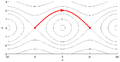  Heteroclinic orbit

Inverse

Inverse = Backward

skipped

• set containing first n iterations of initial point without initial point and its k iterations
• number of elements = n - k

${\mathcal {O}}_{n,k}(z)=\{z_{n-k},z_{n-k+1},\ldots z_{n}\}$

It is used in the average colorings

truncated

• set containing initial point and first n iterations of initial point
• number of elements = n+1

${\mathcal {O}}_{n}(z)=\{z,f(z),\ldots f^{n}(z)\}=\{z_{0},z_{1},\ldots z_{n}\}$

Parameter

Parameter

• point of the parameter plane " is renormalizable if restriction of some of its iterate gives a polinomial-like map of the same or lower degree. "
• parameter of the function

Period

Period of point $z_{0}$ under the iterarted function f is the smallest positive integer value p for which this equality

$f^{p}(z_{0})=z_{0}$

holds is the period of the orbit.

$z_{0}$ is a point of periodic orbit (limit cycle) $\{z_{0},\dots ,z_{p-1}\}$.

More is here

Plane

Planes

Douady’s principle: “sow in dynamical plane and reap in parameter space”.

2-sphere

In topology: two-dimensional sphere = 2-sphere = the two-dimensional surface of a three-dimensional ball

Geometrically, the set of extended complex numbers is referred to as the Riemann sphere or extended complex plane.

partition

Examples:

• Markow
• Yoccoz puzzle

Kneading partition of the dynamic plane

In case of critically preperiodic polynomials the partition of the dynamic plane used in the definition of the kneading sequence.

Partition is formed by the dynamic rays at angles:

• t/2
• (t + 1)/2

which land together at the critical point.

Angle t is angle which lands on the critical value:

$z=c$

• 

  t = 1/4 preperiod = 2 period = 1

• 

  t = 1/6 preperiod = 1 and period = 2

• 

  t = 9/56 preperiod = 3 and period = 3

Spine partition of the dynamic plane

Curve $R\,$:

$R\ {\overset {\underset {\mathrm {def} }{}}{=}}\ R_{1/2}\ \cup \ S_{c}\ \cup \ R_{0}\,$

where:

• R is an dynamic external ray
• S is the spine of Julia set

divides dynamical plane into two components.

• 

  Plane paritition in case of Rabbit Julia set

• 

  Plane paritition in case of Basilica Julia set

crossing/noncrossing

noncrossing: "A partition of a (finite) set is just a subdivision of the set into disjoint subsets. If the set is represented as points on a line (or around the edge of a disc), we can represent the partition with lines connecting the dots. The lines usually have lots of crossings. When the partition diagram has no crossing lines, it is called a non-crossing partition. ... They have a lot of beautiful algebraic structure, and are related to lots of old enumeration problems. More recently (and importantly), they turn out to be a crucial tool in understanding how the eigenvalues of large random matrices behave." Todd Kemp (UCSD)

Key words:

• Enumerative combinatorics

types

• slit plane = plane with the slit deleted: Let S be the "slit plane" $S=\mathbb {C} -\{t\in \mathbb {R} :t\leq 0\}$
• chessboard or checkerboards

types in case of discrete dynamical system

Dynamic plane or phase space

• z-plane for fc(z)= z^2 + c
• z-plane for fm(z)= z^2 + m*z

Parameter plane

See:

Types of the parameter plane:

• c-plane (standard plane)
• exponential plane (map)
• flatten' the cardiod (unroll) = "A region along the cardioid is continuously blown up and stretched out, so that the respective segment of the cardioid becomes a line segment. .." (Figure 4.22 on pages 204-205 of The Science Of Fractal Images)
• transformations

• 

  c-plane

• 

  inverted c plane = 1/c plane

• 

  unrolled

• 

  lambda plane

Points

Band-merging

the band-merging points are Misiurewicz points

Biaccessible

If there exist two distinct external rays landing at point we say that it is a biaccessible point.

blowup point

blowup point = parameter for which the critical orbits map to ∞, so the Julia set is the entire sphere

Buried

" a point of the Julia set is buried if it is not in the boundary of any Fatou component."

polynomials do not have buried points

some rational Julia sets have (Residual Julia Set = Buried Points)

Center

Nucleus or center of hyperbolic component

A center of a hyperbolic component H is a parameter $c_{0}\in H\,$ (or point of parameter plane) such that

• the corresponding periodic orbit has multiplier= 0."
• it has a superstable periodic orbit

Synonyms:

• Nucleus of a Mu-Atom

How to find center/s ?

Center of Siegel Disc

Center of Siegel disc is a irrationally indifferent periodic point.

Mane's theorem:

"... appart from its center, a Siegel disk cannot contain any periodic point, critical point, nor any iterated preimage of a critical or periodic point. On the other hand it can contain an iterated image of a critical point."

Critical

A critical point of $f_{c}\,$ is a point $z_{cr}\,$ in the dynamical plane such that the derivative vanishes:

$f_{c}'(z_{cr})=0.\,$

A critical value is an image of critical point

complex quadratic polynomial

For the complex quadratic polynomial in the c form

$f_{c}'(z)={\frac {d}{dz}}f_{c}(z)=2z$

implies

$z_{cr}=0\,$

we see that the only (finite) critical point of $f_{c}\,$ is the point $z_{cr}=0\,$.

$z_{0}$ is an initial point for Mandelbrot set iteration.

Cut

The "neck" of this eight-like figure is a cut-point.

Cut points in the San Marco Basilica Julia set. Biaccessible points = landing points for 2 external rays

Cut point k of set S is a point for which set S-k is dissconected (consist of 2 or more sets). This name is used in a topology.

Examples:

• root points of Mandelbrot set
• Misiurewicz points of boundary of Mandelbrot set
• cut points of Julia sets (in case of Siegel disc critical point is a cut point)

These points are landing points of 2 or more external rays.

Point which is a landing point of 2 external rays is called biaccesible

Cut ray is a ray which converges to landing point of another ray. Cut rays can be used to construct puzzles.

Cut angle is an angle of cut ray.

fixed

Periodic point when period = 1

Feigenbaum

• 

  Zoom toward Feigenbaum point

• 

  The Feigenbaum point (red arrow) is limit of the bifurcation point

The Feigenbaum Point is a:

• point c of parameter plane
• is the limit of the period doubling cascade of bifurcations
• the accumulation point of the period-doubling cascade in the real-valued x^2+c mapping
• an infinitely renormalizable parameter of bounded type
• boundary point between chaotic (-2 < c < MF) and periodic region (MF< c < 1/4)

$MF^{(n)}({\tfrac {p}{q}})=c$

Generalized Feigenbaum points are:

• the limit of the period-q cascade of bifurcations
• landing points of parameter ray or rays with irrational angles

Examples:

• $MF^{(0)}=MF^{(1)}({\tfrac {1}{2}})=c=-1.401155$
• -.1528+1.0397i)

The Mandelbrot set is conjectured to be self- similar around generalized Feigenbaum points when the magnification increases by 4.6692 (the Feigenbaum Constant) and period is doubled each time

n	Period = 2^n	Bifurcation parameter = cn	Ratio $={\dfrac {c_{n-1}-c_{n-2}}{c_{n}-c_{n-1}}}$
1	2	-0.75	N/A
2	4	-1.25	N/A
3	8	-1.3680989	4.2337
4	16	-1.3940462	4.5515
5	32	-1.3996312	4.6458
6	64	-1.4008287	4.6639
7	128	-1.4010853	4.6682
8	256	-1.4011402	4.6689
9	512	-1.401151982029
10	1024	-1.401154502237
infinity		-1.4011551890 ...

Bifurcation parameter is a root point of period = 2^n component. This series converges to the Feigenbaum point c = −1.401155

The ratio in the last column converges to the first Feigenbaum constant.

" a "Feigenbaum point" (an infinitely renormalizable parameter of bounded type, such as the famous Feigenbaum value which is the limit of the period-2 cascade of bifurcations), then Milnor's hairiness conjecture, proved by Lyubich, states that rescalings of the Mandelbrot set converge to the entire complex plane. So there is certainly a lot of thickness near such a point, although again this may not be what you are looking for. It may also prove computationally intensive to produce accurate pictures near such points, because the usual algorithms will end up doing the maximum number of iterations for almost all points in the picture." Lasse Rempe-Gillen

Fibonacci

Fibonacci point

infinity

The point at infinity " is a superattracting fixed point, but more importantly its immediate basin of attraction - that is, the component of the basin containing the fixed point itself - is completely invariant (invariant under forward and backwards iteration). This is the case for all polynomials (of degree at least two), and is one of the reasons that studying polynomials is easier than studying general rational maps (where e.g. the Julia set - where the dynamics is chaotic - may in fact be the whole Riemann sphere). The basin of infinity supports foliations into "external rays" and "equipotentials", and this allows one to study the Julia set. This idea was introduced by Douady and Hubbard, and is the basis of the famous "Yoccoz puzzle"." Lasse Rempe-Gillen

Mandelbrot set at Fibonacci point

Misiurewicz

Misiurewicz point = " parameters where the critical orbit is pre-periodic.

Myrberg-Feigenbaum

MF = the Myrberg-Feigenbaum point is the different name for the Feigenbaum Point.

Parabolic point

parabolic points: this occurs when two singular points coalesce in a double singular point (parabolic point)

"the characteristic parabolic point (i.e. the parabolic periodic point on the boundary of the critical value Fatou component) of fc"

Periodic

Point z has period p under f if:

$z:\ f^{p}(z)=z$

In other words point is periodic

See also:

• fixed point
• stability of periodic point
  • attracting
  • repelling
  • indifferent
• multiplier of periodic cycle

Pinching

"Pinching points are found as the common landing points of external rays, with exactly one ray landing between two consecutive branches. They are used to cut M or K into well-defined components, and to build topological models for these sets in a combinatorial way. " (definition from Wolf Jung program Mandel)

other names

• pinch points
• cut points

See for examples:

• period 2 = Mandel, demo 2 page 3.
• period 3 = Mandel, demo 2 page 5

Pool

"A point in the dendrite is called a pool if it is the landing point for two external rays, both of whose angles are of the form

${\frac {k}{12*2^{n}}}$

for some k, n ∈ N, where k ≡ 1 mod 6.

...

central pool ... it is geometrically the center of the dendrite; a one half rotation around this point maps the dendrite to itself."

post-critical

A post-critical point is a point

$z=f(f(f(...(z_{cr}))))$

where $z_{cr}$ is a critical point.

See also:

• post-critical set

precritical

precritical points, i.e., the preimages of the critical point

reference point

Reference point of the image:

• its orbit (reference orbit) is computed with arbitrary precision and saved
• orbits of the other points of the image (no-reference points) are computed from reference orbit using standard precision (with hardware floating point numbers) = faster then using arbitrary precision

renormalizable

point of the parameter plane " is renormalizable if restriction of some of its iterate gives a polinomial-like map of the same or lower degree. "

infinitely renormalizable

" a "Feigenbaum point" (an infinitely renormalizable parameter of bounded type, such as the famous Feigenbaum value which is the limit of the period-2 cascade of bifurcations), then Milnor's hairiness conjecture, proved by Lyubich, states that rescalings of the Mandelbrot set converge to the entire complex plane. So there is certainly a lot of thickness near such a point, although again this may not be what you are looking for. It may also prove computationally intensive to produce accurate pictures near such points, because the usual algorithms will end up doing the maximum number of iterations for almost all points in the picture." Lasse Rempe-Gillen

IMMEDIATE RENORMALIZATION

" A cubic polynomial P with a non-repelling fixed point b is said to be immediately renormalizable if there exists a (connected) quadratic-like invariant filled Julia set K∗ such that b ∈ K∗ . In that case exactly one critical point of P does not belong to K∗."

repelling

Virtually repelling

virtually repelling fixed points

root or bond

The root point of the hyperbolic component of the Mandelbrot set:

• A point where two mu-atoms meet
• has a rotational number 0
• it is a biaccesible point (landing point of 2 external rays)

Names:

• bond

singular

the singular points of a dynamical system

In complex analysis there are four classes of singularities:

• Isolated singularities: Suppose the function f is not defined at a, although it does have values defined on U \ {a}.
  • The point a is a removable singularity of f if there exists a holomorphic function g defined on all of U such that f(z) = g(z) for all z in U \ {a}. The function g is a continuous replacement for the function f.
  • The point a is a pole or non-essential singularity of f if there exists a holomorphic function g defined on U with g(a) nonzero, and a natural number n such that f(z) = g(z) / (z − a)ⁿ for all z in U \ {a}. The least such number n is called the order of the pole. The derivative at a non-essential singularity itself has a non-essential singularity, with n increased by 1 (except if n is 0 so that the singularity is removable).
  • The point a is an essential singularity of f if it is neither a removable singularity nor a pole. The point a is an essential singularity if and only if the Laurent series has infinitely many powers of negative degree.
• Branch points are generally the result of a multi-valued function, such as ${\sqrt {z}}$ or $\log(z)$ being defined within a certain limited domain so that the function can be made single-valued within the domain. The cut is a line or curve excluded from the domain to introduce a technical separation between discontinuous values of the function. When the cut is genuinely required, the function will have distinctly different values on each side of the branch cut. The shape of the branch cut is a matter of choice, however, it must connect two different branch points (like $z=0$ and $z=\infty$ for $\log(z)$) which are fixed in place.

tip

• from Mu-Ency: "the point in a primary filament that has the simplest external angle; this is the point that you get by appending FS[(1/2B1)] an infinite number of times to the primary filament's name." This is also the "limit" of the ... series.
• Misurewicz point

• 

  tip of the main antenna (1/2 wake) $c=M_{1,1}$

• 

triple

"A point in the dendrite is called a triple point if its removal separates the dendrite into three connected components. Such a point is the landing point for three external rays, whose angles all have of the form

${\frac {k}{7*2^{n}}}$

for some k, n ∈ N, where k is congruent to 1, 2 or 4, mod 7." Will Smith in Thompson-Like Groups for Dendrite Julia Sets

Portrait

orbit portrait

types

There are two types of orbit portraits: primitive and satellite. If $v$ is the valence of an orbit portrait ${\mathcal {P}}$ and $r$ is the recurrent ray period, then these two types may be characterized as follows:

• Primitive orbit portraits have $r=1$ and $v=2$. Every ray in the portrait is mapped to itself by $f^{n}$. Each $A_{j}$ is a pair of angles, each in a distinct orbit of the doubling map. In this case, $r_{\mathcal {P}}$ is the base point of a baby Mandelbrot set in parameter space.
• Satellite (non-primitive) orbit portraits have $r=v\geq 2$. In this case, all of the angles make up a single orbit under the doubling map. Additionally, $r_{\mathcal {P}}$ is the base point of a parabolic bifurcation in parameter space.

Critical

Critical orbit portrait = portrait of the critical orbit

... for the polynomial $z\to z^{2}+i$ we may note the critical orbit portrait:

$0\to i\to -1+i\to -i\to -1+i$

for this map, or we may double the angles of external rays and record the locations of landing points in order to observe the same behavior."

Precision

Precision of:

• data type used for computation. Measured in bits (width of significant (fraction) = number of binary digits) or in decimal digits
• input values
• result (number of significant figures)

See:

• Numerical Precision: " Precision is the number of digits in a number. Scale is the number of digits to the right of the decimal point in a number. For example, the number 123.45 has a precision of 5 and a scale of 2."
• error

Principle

Douady’s principle

Douady’s principle: “sow in dynamical plane and reap in parameter space”.

Problem

small divisor problem

Types

• One-Dimensional Small Divisor Problems (On Holomorphic Germs and Circle Diffeomorphisms)
• linearization problem in complex dimension one dynamical systems: "Given a fixed point of a differentiable map, seen as a discrete dynamical system, the linearization problem is the question whether or not the map is locally conjugated to its linear approximation at the fixed point. Since the dynamics of linear maps on finite dimensional real and complex vector spaces is completely understood, the dynamics of a map on a finite dimensional phase space near a linearizable fixed point is tractable."

Where it can be found:

• stability in mechanics, particularly in celestial mechanics
• relations between the growth of the entries in the continued fraction expansion of t and the behaviour of f around z=0 under iteration.

See:

• Linearization in scholarpedia

Processes or transformations and phenomenona

Aliasing and antialiasing

• aliasing

Conjugation

Topological conjugacy

two functions are said to be topologically conjugate if there exists a homeomorphism that will conjugate the one into the other. Topological conjugacy also known as topological equivalence is important in the study of iterated functions and more generally dynamical systems, since, if the dynamics of one iterative function can be determined, then that for a topologically conjugate function follows trivially.

To illustrate this directly: suppose that $f$ and $g$ are iterated functions, and there exists a homeomorphism $h$ such that

$g=h^{-1}\circ f\circ h,$

so that $f$ and $g$ are topologically conjugate. Then one must have

$g^{n}=h^{-1}\circ f^{n}\circ h,$

and so the iterated systems are topologically conjugate as well. Here, $\circ$ denotes function composition.

Commutative square diagram

• a collection of maps
• square diagram that commutes = all map compositions starting from the same set A and ending with the same set D give the same result

Examples

• The logistic map and the tent map are topologically conjugate.
• The logistic map of unit height and the Bernoulli map are topologically conjugate.^{[citation needed]}
• For certain values in the parameter space, the Hénon map when restricted to its Julia set is topologically conjugate or semi-conjugate to the shift map on the space of two-sided sequences in two symbols.

Contraction and dilatation

• the contraction z → z/2
• the dilatation z → 2z.

convolution

In the digital image processing: image convolution Convolution is used to

• extract certain features from an input image, like edge

Image convolutions by dimensions of the kernel array:

• 1D
  • LIC
• 2D
  • Gaussian blur (Gaussian smoothing)
  • Sobel filter

See also

• feature detection (Feature extraction)
  • edge detection
  • Ridge detection
  • Motion detection
  • Blob detection

differentiation

Method of computing the derivative of a mathematical function

types:

• symbolic differentiation
• Automatic Differentiation (AD)
• numeric differentiation = the method of finite differences

Discretizations

• discretization and its reverse
• discretize/homogenize in the DDG (Discrete Differential Geometry)

Discretization is the process of transferring continuous functions, models, variables, and equations into discrete counterparts.

Examples:

• Cartesian coordinate system ( regular grid ) of continous space

distorsion

• distorsion of the plane = plane transformation
• distortion of Mandelbrot set island

Implosion and explosion

Explosion (above) and implosion (below)

Implosion is:

• the process of sudden change of quality fuatures of the object, like collapsing (or being squeezed in)
• the opposite of explosion

Example:

• parabolic implosion in complex dynamics (${\mathbf {C}}$)
  • when filled Julia for complex quadratic polynomial set looses all its interior (when c goes from 0 along internal ray 0 thru parabolic point c=1/4 and along extrnal ray 0 = when c goes from interior, crosses the boundary to the exterior of Mandelbrot set)
  • " We can see that $J_{{\frac {1}{4}}+.0005}$ looks somewhat like $J_{\frac {1}{4}}$ from the "outside", but on the "inside" there are curlicues; pairs of them are vaguely reminiscent of "butterflies". As t→0, these butterflies persist and remain uniformly large. We think of t as representing time, which decreases to 0. The fact that they suddenly disappear for t=0 is the phenomenon called "implosion". Or, if we think of time starting at t=0, then the instantaneous appearance of large "butterflies" for t>0 may be thought of as "explosion". "
  • the Julia set implodes when under small perturbations (epsilon) near parabolic parameter (like c = 1/4)
• Semi-parabolic implosion in ${\mathbf {C}}^{2}$

• Implosion: from circle thru cauliflower to imploded cauliflower
• 
• 
• 

Explosion is a:

• sudden change of quality fuatures of the object in an extreme manner,
• the opposite of implosion

Example: in exponential dynamics when λ> 1/e, the Julia set of $E_{\lambda }(z)=\lambda e^{z}$ is the entire plane.

integrating

• integrating along some vector field means finding a solution curve. Example: finding extrrernal ray using Runge-Kutta method for numerical integration

Linearization

• changing from non-linear to linear
• " ... turn the perturbated linear map $f:\lambda z+z^{2}\mapsto \lambda z$ into the exactly linear map $y\mapsto \lambda y$ (it linearizes $f$)" Jean-Christophe Yoccoz
• linearization in english wikipedia
• Linearization in scholarpedia
• "System is linearizable at the origin if and only if there exists a change of coordinates which linearizes the system, that is, all the coefficients of the normal form vanish."

Linearization with inverse function

Examples:

• Parabolic Linearization

Mating

Mating

Normalization

Normalize

• normalize = transformation to the model
• " normalize this vector so it has modulus one " A Cheritat
• move fixed point to the origin (z = 0)
• mapping the range of variable to standard range
  • [0.0, 1.0]
  • [0,255], like rgb values
• converting closed curve to unit circle
• converting closed curves to concentric circles with center at the origin

See also:

• uniformization
• renormalization

Parametrization

• Parametrization is the process of finding parametric equations of a curve

Perturbation

• Perturbation technque for fast rendering the deep zoom images of the Mandelbrot set
• perturbation of parabolic point
• use perturbation theory to approximate the solutions of the differential equations
• perturbation of point x: $x\to x+\epsilon$ where epsilon is absolute value of approximation error
• adding some small value ( epsilon denoted by Greek letter $\epsilon$) to the constant value to see how function changes near hard to analyze values

Separation

• "the double fixed point 0 of $f_{\epsilon }$ usually splits into two fixed points. ... These points separate at some speed" ( PARABOLIC IMPLOSION. A MINI-COURSE by ARNAUD CHERITAT )

Renormalization

"to any quadratic map f we can associate a canonical sequence of periods p1 < p2 <... for which f is renormalizable.

Depending on whether the sequence is:

• empty
• finite
• infinite

the map f is called respectively:

• non-renormalizable
• at most finitely renormalizable
• infinitely renormalizable"

"Sectorial renormalizations are useful in the nonlinearizable situation. " Ricardo Pérez-Marco

The self-similarity is a result of something called "renormalization" (which as far as I know is not related to the concept with the same name in quantum field theory). Jim Belk

Examples:

• Near parabolic renormalization for unicritical holomorphic maps
• how theories change as we move to more or less detailed descriptions is known as renormalization. by Simon DeDeo

Surgery

• surgery in differential topology
• regluing

• 

  Surgery on the circle

• 

  Surgery on the sphere

Links:

• http://mathoverflow.net/questions/tagged/surgery-theory

Tuning

• definition
• examples
  • subwake
  • island

Uniformization

Uniformization of 

• Hyperbolic Components of Mandelbrot set to the unit disc = multiplier map
• basin of superattractive fixed point - Bottcher map (The Bottcher uniformization theorem)

property or feature

behavior

• local behavior is the behavior of a complex analytic function near some point (fixed, periodic) = Local theory of periodic orbits = local dynamics
• global behavior

Density

density of the image

Dense image

• downsaling with gamma correction
• path finding
• supersampling: "ots of detail but fractal fades away as you get more accurate, as n increases in nxn supersampling" TGlad

Hyperbolic/parabolic/eliptic

The meaning of the terms "elliptic, hyperbolic, parabolic" in different disciplines in mathematics

• PDE (Linear Second Order PDE’s in two Independent Variables):
• Moebius transformations:
• Discrete local complex dynamics
• Conic section
• Quadratic form
• Probability distributions.

Invariant

sth is invariant with respect to the transformation = non modified, steady

Topological methods for the analysis of dynamical systems

Invariants type

• metric invariants
• dynamical invariants,
• topological invariants.

dynamical

Dynamical invariants = invariants of the dynamical system

• periodic points
  • fixed point
• invariant curve
  • periodic ray
    • external: fixed curves near fixed point
    • internal

Dynamical Invariants Derived from Recurrence Plots

Orientation

• A compass rose: Notice that the convention for measuring angles is different to the convention we used in the unit circle definition of the trigonometric functions.
  • Firstly 0o is North, rather than the x axis.
  • Secondly the direction in which angles increase is clockwise rather than counter-clockwise.
• Unit circle :
  • the direction in which angles increase is counter-clockwise
  • angle zero is the x axis direction
• Cartesian coordinate system

• 
• 
• 

smooth

smooth = changing without visible (noticeable) edges

use:

• smooth gradient

similar:

• continuous

compare:

• discrete

Stability

• stability of quasiperiodic motion under small perturbation. In the celestial mechanics dynamics of 3 bodies around sun is described by the system of differential equations. In such case it "becomes fantastically complicated and remains largely mysterious even today." See KAM = Kolmogorov–Arnold–Moser theorem and small divisor problem
• stability of the fixed point under small perturbation
• there is equivalence (for |f′(0)| ≤ 1) of stability (a topological notion) and linearizability (an analytical notion)

Compare with:

• shadowing lemma
• Sensitive dependence on initial conditions - Butterfly effect

Radius

Radius of complex number

The absolute value or modulus or magnitude or radius of a complex number

Conformal radius

Conformal radius of Siegel Disk

Escape radius (ER)

Escape radius (ER) or bailout value is a radius of circle centered at origin (z=0). This set is used as a target set in the bailout test (escape time method = ETM)

Minimal

Minimal Escape Radius should be grater or equal to 2:

$ER=max(2,|c|)\,$

Better estimation is:

$ER={\frac {1}{2}}+{\sqrt {{\frac {1}{4}}+|c|}}$

crossing

How to choose parameters for which level curves cross critical point (and its preimages)? Choose escape radius equal to n=th iteration of critical value.

• level curves cross at critical point
• 

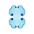  not cross

• 

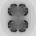  cross

• 

  cross

// find such ER for LSM/J that level curves croses critical point and it's preimages
double GiveER(int i_Max){

	complex double z= 0.0; // critical point
	int i;
	 ; // critical point escapes very fast here. Higher valus gives infinity
	for (i=0; i< i_Max; ++i ){
		z=z*z +c; 
	 
	 }
	 
	 return cabs(z);
	
	
}

Another way: choose the parameter c such that it is on an escape line, then the critical value will be on an escape line as well.

Inner radius

Inner radius of Siegel Disc

• radius of inner circle, where inner circle with center at fixed point is the biggest circle inside Siegel Disc.
• minimal distance between center of Siel Disc and critical orbit

Internal radius

Internal radius is a:

• absolute value of multiplier $r=|\lambda |$

See also: the N-2 rule

Sequences

A sequence is an ordered list of objects (or events).

A series is the sum of the terms of a sequence of numbers. Some times these names are not used as in above definitions.

Itinerary

$S(x)$ is an itinerary of point x under the map f relative to the paritirtion.

It is a right-infinite sequence of zeros and ones

 $S(x)=s_{1}s_{2}s_{3}...s_{n}$

where

Examples:

• internal angle and wake

For rotation map $R_{p/q}$ and invariant interval $I$ (circle):

$I=(0,1]$

one can compute $x_{c}$:

 $x_{c}=1-{\frac {p}{q}}$

and split interval into 2 subintervals (lower circle partition):

$I_{0}=(0,x_{c}]$

$I_{1}=(x_{c},1]$

then compute s according to it's relation with critical point:

$s_{n}={\begin{cases}0:x_{n}<x_{c}\\1:x_{n}>x_{c}\end{cases}}$

Itinerary can be converted to point $x\in [0,1]$

$\gamma (S_{n})=0.s_{1}s_{2}s_{3}...s_{n}=\sum _{n=0}^{n-1}{\frac {s_{n}}{2^{n}}}=x_{n}$

kneading sequence

• "the kneading sequence of an external angle ϑ (here ϑ = 1/6) is defined as the itinerary of the orbit of ϑ under angle doubling, where the itinerary is taken with respect to the partition formed by the angles ϑ/2, and (ϑ + 1)/2 "
• The itinerary ν = ν1ν2ν3 . . . of the critical value is called the kneading sequence. One can start from the critical point but neglect the initial symbol. Such sequence is computed with the Hubbard tree

• Paritition of dynamic plane related with kneading sequence
• 

  1/4

• 

  1/6 preperiod = 1 and period = 2

• 

  9/56 preperiod = 3 and period = 3

• 

  129/16256

See also:

• kneading theory
• Milnor–Thurston_kneading_theory in wikipedia
• combinatorial dynamics

Thue–Morse sequence

Thue–Morse sequence

• how to compute it

Orbit

Orbit can be:

• forward = sequence of points
• backward (inverse)
  • tree in case of multivalued function
  • sequence

Series

A series is the sum of the terms of a sequence of numbers. Some times these names are not used as in above definitions.

Taylor

• Taylor series and Mandelbrot set
• The Existence and Uniqueness of the Taylor Series of Iterated Functions

Set

Attracting set

Informal definition:

  "an attracting set for a dynamical system is a closed subset A of its phase space such that for "many" choices of initial point the system will evolve towards A ." John W Milnor

Continuum

definition

Band

chaotic band

Chaotic bands from B0 to B10

period-$2^{n}$ chaotic band $B_{n}$

• is between Misiurewicz points (primary separators) $m_{n}$ and $m_{n+1}$
• it's biggest midget has period $3*2^{n}$
• contains Sharkovsky subsequence: sequence of islands for periods: $(2k+1)\cdot 2^{n}$ for k = 1, 2, ..... (in the increasing order = increasing from left to right). These are first appearance of hyperbolic components with such period in Sharkowsky ordering
• is on n-place in Sharkowsky ordering

$m_{n}\prec B_{n}\prec m_{n+1}$

$m_{n}\prec (2k+1)\cdot 2^{n}\prec m_{n+1}$

$m_{n}\prec (2+1)\cdot 2^{n}\prec (4+1)\cdot 2^{n}\prec (6+1)\cdot 2^{n}\prec ...\prec m_{n+1}$

${\begin{array}{cccccccc}3&5&7&9&11&\ldots &(2n+1)\cdot 2^{0}&\ldots \\3\cdot 2&5\cdot 2&7\cdot 2&9\cdot 2&11\cdot 2&\ldots &(2n+1)\cdot 2^{1}&\ldots \\3\cdot 2^{2}&5\cdot 2^{2}&7\cdot 2^{2}&9\cdot 2^{2}&11\cdot 2^{2}&\ldots &(2n+1)\cdot 2^{2}&\ldots \\3\cdot 2^{3}&5\cdot 2^{3}&7\cdot 2^{3}&9\cdot 2^{3}&11\cdot 2^{3}&\ldots &(2n+1)\cdot 2^{3}&\ldots \\\vdots \\MF\end{array}}$

Dwell bands

"Dwell bands are regions where the integer iteration count is constant, when the iteration count decreases (increases) by 1 then you have passed a dwell band going outwards (inwards). " Other names:

• level sets of integer escape time

Basin

Basin can consist of

• one component, like basin of infinity

of attraction

definitions:

• An attractor's basin of attraction is the region of the phase space, over which iterations are defined, such that any point (any initial condition) in that region will asymptotically be iterated into the attractor
• The collection of all points whose iterates under f converge to the attractor

immediate basin of attraction

the component of the basin containing the periodic point itself

Examples

• basin of infinity (whole basin = one component)

$$A_{f}(\infty )\ {\overset {\underset {\mathrm {def} }{}}{=}}\ \{z\in \mathbb {C} :f^{(k)}(z)\to \infty \ as\ k\to \infty \}.$$

• 

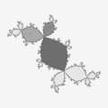  1/3

• 

  3/17

Component

Components of parameter plane

Names:

• mu-atom
• ball
• bud
• bulb
• decoration: "A decoration of the Mandelbrot set M is a part of M cut off by two external rays landing at some tip of a satellite copy of M attached to the main cardioid."
• lake
• lakelet.

filament

from Mu-Ency: "Any contiguous subset of the Mandelbrot Set which consists of the infinitely convoluted and branching structures that connect the island mu-molecules to each other."

Some colloquial names for filaments:

• antenna
  • main antenna
• spike
• spoke.

 "A filament consists of a) minibrots and b) limit points of sequences of those minibrots. The latter include Misiurewicz points (rational external angles, one for filament termini and two or more for interior points such as multi-armed spiral centers) and other points (with irrational external angles).
 My intuition says if you zoom to a succession of smaller minis along a filament, if this is done in a pattern for infinitely long you tend to a Misiurewicz point, and if it's done randomly for infinitely long you tend to an irrational point. But I have no proof of this. 
 Other noninterior points on filaments mostly belong to individual minibrots: cardioid cusps (two rational external angles, odd denominator) and minibrot-filament branch tips (Misiurewicz points, two rational external angles, even denominator). 
 There is one last point: the exact base of the filament where it attaches to something (minibrot or main set). This point has irrational external angles. The Feigenbaum point at the base of the spike is one of these." pauldelbrot

Islands

Names:

• mini Mandelbrot set
• 'baby'-Mandelbrot set
• island mu-molecules = embedded copy of the Mandelbrot Set
• Bug
• Island
• Mandelbrotie
• Midget

List of islands:

• http://mrob.com/pub/mu-data/largest-islands.txt
• http://mrob.com/pub/muency/largestislands.html
• http://www.math.cornell.edu/~rperez/Documents/maximals.pdf
• http://fraktal.republika.pl/mset_external_ray_mini.html
• http://mathr.co.uk/mandelbrot/feature-database.csv.bz2 (a database of all islands up to period 16, found by tracing external rays): period, islandhood, angled internal address, lower external angle numerator, denominator, upper numerator, denominator, orientation, size, centre realpart, imagpart

features of island

• period
• symbolic sequence
• angled internal address
• lower and upper external angle of rays landing on it's root
• center (
• root
• orientation
• size
• distortion
• tip (Misiurewicz point,
  • c value
  • period and preperiod
  • lower and upper external angle of rays landing on it

Primitive and satellite

"Hyperbolic components come in two kinds, primitive and satellite, depending on the local properties of their roots."

• primitive (non-satellite)
  • the root of component is not on the boundary of another component = "it was born from another hyperbolic component by the period increasing bifurcation"
  • ones that have a cusp likes the main cardioid, when the little Julia sets are disjoint
• satellite
  • ones that don't have a cusp
  • it's root is on the boundary of another hyperbolic component
  • when the little Julia sets touch at their β-fixed point

Child (Descendant) and the parent (ancestor)

• ancestor of hyperbolic component
• descendant of hyperbolic component = child

Hyperbolic component of Mandelbrot set

Boundaries of hyperbolic components of Mandelbrot set

Domain is an open connected subset of a complex plane.

"A hyperbolic component H of Mandelbrot set is a maximal domain (of parameter plane) on which $f_{c}\,$ has an attracting periodic orbit.

A center of a H is a parameter $c_{0}\in H\,$ (or point of parameter plane) such that the corresponding periodic orbit has multiplier= 0."

A hyperbolic component is narrow if it contains no component of equal or lesser period in its wake

features of hyperbolic component

• period
• islandhood (shape = cardiod or circle)
• angled internal address
• lower and upper external angle of rays landing on it's root
• center (
• root
• orientation
• size

Abreviations:

• LAHCs = the last appearance HCs placed in the chaotic region

Limb

• The part of the Mandelbrot set contained in the wake together with the root $c_{H}$ is called the limb $L_{H}$ of the Mandelbrot set originated at H (hyperbolic component of the Mandelbrot set)

13/34 limb and wake on the left image

p/q-limb is a part of Mandelbrot set contained inside p/q-wake

For every rational number ${\tfrac {p}{q}}$, where p and q are relatively prime, a hyperbolic component of period q bifurcates from the main cardioid. The part of the Mandelbrot set connected to the main cardioid at this bifurcation point is called the p/q-limb. Computer experiments suggest that the diameter of the limb tends to zero like ${\tfrac {1}{q^{2}}}$. The best current estimate known is the Yoccoz-inequality, which states that the size tends to zero like ${\tfrac {1}{q}}$.

A period-q limb will have q − 1 "antennae" at the top of its limb. We can thus determine the period of a given bulb by counting these antennas.

In an attempt to demonstrate that the thickness of the p/q-limb is zero, David Boll carried out a computer experiment in 1991, where he computed the number of iterations required for the series to converge for z = $-{\tfrac {3}{4}}+i\epsilon$ ($-{\tfrac {3}{4}}$ being the location thereof). As the series doesn't converge for the exact value of z = $-{\tfrac {3}{4}}$, the number of iterations required increases with a small ε. It turns out that multiplying the value of ε with the number of iterations required yields an approximation of π that becomes better for smaller ε. For example, for ε = 0.0000001 the number of iterations is 31415928 and the product is 3.1415928.

Types:

• The limbs attached to the main cardioid are called primary.
• Let H be a hyperbolic component attached to the main cardioid. The limbs attached to such a component are called secondary
• We refer to a truncated limb if we remove from it a neighborhood of its root

molecule

• The main molecule is the union of all hyperbolic components attached to the main cardioid through a chain of finitely many components.
• island mu-molecule = island mu-unit

shrub

• "what emerges from Myrrberg-Feigenbaum point is what we denominate a shrub due to its shape" M Romera
• filament,
• chaotic part of the p/q limb: "The chaotic region is made up of an infinity of hyperbolic components mounted on an infinity of shrub branches in each one of the infinity shrubs of the family."

Examples

• main antenna is a shrub of $F_{1/2}$ family

spokes

"Colloquial term for a filament, specifically one of the "arms" radiating from a branch point." - from Mu-Ency

Wake

Wakes of Mandelbrot Set to Period 10

p/q-wake is the region of parameter plane enclosed by two external rays landing on the same root point on the boundary of main cardioid (period 1 hyperbolic component).

Angles of the external rays that land on the root point one can find by:

• Combinatorial algorithm = Devaney's method
• book program by Claude Heiland-Allen
• wake function from program Mandel by Wolf Jung

p/q-Subwake of W is a wake of a p/q-satellite component of W

Wake 1/3 (bounded by 2 external rays) and internal ray 1/3

wake is named after:

• rotation number p/q (as above)
• angles of external rays landing in it's root point: "If two M-rays $R_{M}(\theta \pm )$ land at the same point $c_{0}$ we denote by wake $(\theta \pm )$ the component of $\mathbb {C} \setminus R_{M}(\theta +)\cup R_{M}(\theta -)\cup \{c_{0}\}$ which does not contain 0."

Components of dynamical plane

• Fatou set components
• components of interior of Julia sets

• 

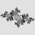  superattracting

• 

  parabolic

• 

  Inverse iteration of Siegel disc component

In case of Siegel disc critical orbit is a boundary of component containing Siegel Disc.

For a quadratic polynomial with a parabolic orbit, the unique Fatou component containing the critical value will be called the characteristic Fatou component; (Dierk Schleicher in Rational Parameter Rays of the Mandelbrot Set)

 "for rational maps (iterating maps of the form f(x)=p(x)/q(x) where p,q are polynomials) result in 1, 2 or infinitely many components."

See also:

• interior and exterior of filled Julia set for polynomials
• immediate basin of attraction

Domain

Domain in mathematical analysis it is an open connected set

Jordan domain

"A Jordan domain J is the homeomorphic image of a closed disk in E2. The image of the boundary circle is a Jordan curve, which by the Jordan Curve Theorem separates the plane into two open domains, one bounded, the other not, such that the curve is the boundary of each."

Examples:

• Petal of the Leau-Fatou flower

Flower

Lea-Fatu flower

Interval

a partition of an interval into subintervals

• Markov partition

Invariant

sth is invariant if it does't change under transformation

"A subset S of the domain Ω is an invariant set for the system (7.1) if the orbit through a point of S remains in S for all t ∈ R. If the orbit remains in S for t > 0, then S will be said to be positively invariant. Related definitions of sets that are negatively invariant, or locally invariant, can easily be given"

Examples:

• invariant set
• invariant point = fixed point
• invariant cycle = periodic point
• invariant curve
  • invariant circle
• petal = invariant planar set

Julia set

Feigenbaum Julia set

Julia set for Feigenbaum parameter c

Successive zooms lead to a Julia set which grows more and more hairs. (Similarly, the Mandelbrot set gains more decorations while limiting on the Feigenbaum point.)
This leads to the natural question: Does the Julia set of the Feigenbaum quadratic polynomial have positive or zero measure?
If zero, is its Hausdorff dimension less than 2?

Level set

• a level set of a real-valued function f (see also dwell band)
• Level set methods (LSM)
  • on the dynamic plane

in case of:

• dynamic plane
• integer escape time
• target set: exterior of the circle (used in the escaping test)

attracting case

On the dynamic plane level set is defined:

$L_{n}=\{z_{0}:abs(z_{n-1})<ER<abs(z_{n})\}\,$

Boundaries of level sets (lemniscates) are

 $B_{n}=\{z_{0}:abs(z_{n-1})=ER\}\,$   

On the parameter plane

$B_{n}=\{c:\operatorname {abs} (z_{n})=ER\}\,$

where

• $ER\,$ is Escape Radius, bailout value, radius of circle which is used to measure if orbit of $z_{0}\,$ is bounded; it is integer number
• $z,c\,$ are complex numbers (points of 2-D planes)
• $z\,$ is point of dynamical plane (z-plane)
• $c\,$ is point of parameter plane (c-plane)
• $c=x+y*i\,$
• $z_{n+1}=f_{c}(z_{n})\,$
• $f_{c}(z)=z^{2}+c\,$
• $z_{0}=0\,$ critical point of $f_{c}\,$

Then:

$B_{1}=\{c:\operatorname {abs} (c)=ER\}=\{(x+y*i):\operatorname {sqrt} (x^{2}+y^{2})=ER\}\,$

$B_{2}=\{c:\operatorname {abs} (c^{2}+c)=ER\}=\{(x+y*i):\operatorname {sqrt} ((-y^{2}+x^{2}+x)^{2}+(2*x*y+y)^{2})=ER\}\,$

$B_{3}=\{c:\operatorname {abs} ((c^{2}+c)^{2}+c)=ER\}=\{(x+y*i):\operatorname {sqrt} ((y^{4}-6*x^{2}*y^{2}-6*x*y^{2}-y^{2}+x^{4}+2*x^{3}+x^{2}+x)^{2}+(-4*x*y^{3}-2*y^{3}+4*x^{3}*y+6*x^{2}*y+2*x*y+y)^{2})=ER\}\,$

...

$B_{1}\,$ is a circle,

$B_{2}\,$ is an Cassini oval,

$B_{3}\,$ is a pear curve.

These curves tend to boundary of Mandelbrot set as n goes to infinity.

• If ER < 2 they are inside Mandelbrot set.
• If ER = 2 curves meet together (have common point) c = −2. Thus they can't be equipotential lines.
• If ER ≥ 2 they are outside of Mandelbrot set. They can also be drawn using Level Curves Method.
• If ER >> 2 they approximate equipotential lines (level curves of real potential, see CPM/M).

• LSM/M
• 

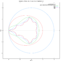  lemniscates of Mandelbrot set

• 

  LCM/J; ER=1000

• 

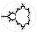  LCM/J but better algorithm, ER = 2

• 

  LSM/J B&W; ER = 1000

• 

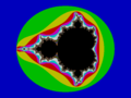  LSM/J colour (probably made with Fractint); ER = 2

parabolic case

• 

$\left|z_{n}-z_{f}\right|=d$

Where:

• d is a diameter of circle
  • through 2 points: $z_{n}$ and $z_{f}$
  • radius r is half of diameter: $r=d/2$
• $z_{n}=f^{p*n}(z_{cr})$ is n*p iteration of critical point
• fixed point of p iteration of f function $z_{f}:z_{f}=f^{p}(z_{f})$
• p is a period of the cycle

Locus

Cantor

The Cantor locus is the unique hyperbolic component, in the moduli space of quadratic rational maps rat2, consisting of maps with totally disconnected Julia sets

Connectedness

In one-dimensional complex dynamics, the connectedness locus is a subset of the parameter space of rational functions, which consists of those parameters for which the corresponding Julia set is connected. the Mandelbrot set is a subset of the complex plane that may be characterized as the connectedness locus of a family of polynomial maps.

Planar set

a non-separating planar set is a set whose complement in the plane is connected.

postsingular

"The postsingular set P(f) of a meromorphic function f is the closure of the union of forward iterates of the singular set S(f):"

${\overline {\cup _{n=0}^{\infty }f^{n}(S(f))}}$

post-critical

• the iterates of the critical set
• "For a rational map of the Riemann sphere f, the post-critical set PC(f) is defined as closure of orbits of all critical points of f. It is proved by Lyubich [Ly83b] that the post-critical set of a rational map is the measure theoretic attractor of points in the Julia set of that map. That is, for every neighborhood of the post-critical set, orbit of almost every point in the Julia set eventually stays in that neighborhood"
• "The postcritical set P(f) of a rational map f is the smallest forward invariant subset of that contains the critical values of f."
• "The analysis of the post-critical set plays a central role in the dynamics of rational maps, mainly because of the following two properties:
  • the set of attracting cycles is always finite for rational maps f
  • every attracting cycle attracts the orbit of a critical point of f."

region

• Shell-Thron region

Sepal

Sepal

Singular set

"The singular set S(f) of a meromorphic function f : C → Cˆ is the collection of values w at which one can not define all branches of the inverse f −1 in any neighborhood of w. If f is rational, then S(f) coincides with the collection of critical values of f. If f is transcendental meromorphic, f −1 may also fail to be defined in a neighborhood of an asymptotic value"

Target set

Target set

• trap for forward orbit
• it is a set which captures any orbit tending to fixed / periodic point

Trap

Trap is another name of the target set

Test

Bailout test or escaping test

Two sets after bailout test: escaping white and non-escaping black

Distance to fixed point for various types of dynamics

It is used to check if point z on dynamical plane is escaping to infinity or not. It allows to find 2 sets:

• escaping points (it should be also the whole basing of attraction to infinity)
• not escaping points (it should be the complement of basing of attraction to infinity)

In practice for given IterationMax and Escape Radius:

• some pixels from set of not escaping points may contain points that escape after more iterations then IterationMax (increase IterMax)
• some pixels from escaping set may contain points from thin filaments not choosed by maping from integer to world (use DEM)

If $z_{n}$ is in the target set $T\,$ then $z_{0}$ is escaping to infinity (bailouts) after n forward iterations (steps).

The output of test can be:

• boolean (yes/no)
• integer: integer number (value of the last iteration)

Types of bailout test:

• in Fractalzoom
• other description
• kf - p-norm with weights

Criterion

criterion = an algorithm which will always give an answer

Theorem

• The Douady-Hubbard landing theorem for periodic external rays of polynomial dynamics: "for a complex polynomial f with bounded postcritical set, every periodic external ray lands at a repelling or parabolic periodic point, and conversely every repelling or parabolic point is the landing point of at least one periodic external ray."