Fractals/Iterations in the complex plane/boettcher

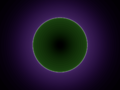
The Böttcher function of which maps the complement of the Mandelbrot set ( Julia set) conformally to the complement of the closed unit disk.

Complex potential on the parameter plane

Gradient of the potential

Complex potential

Complex potential on dynamical plane

Let $p(z)$ be a polynomial with degree d and $\ln ^{+}(x)=\max\{0,ln(x)\}.$ Then Green's function $G_{p}$ for polynomial p is:

$G_{p}(z):=\lim _{n\to \infty }{\frac {1}{d^{n}}}\ln ^{+}|p^{\circ n}|$

Exterior or complement of filled-in Julia set is :

• a basin of attraction of infinity ( superattracting fixed point) so dynamics in ttah basin is the same for all polynomials !!!
• one of components of the Fatou set

$A_{f_{c}}(\infty )=K(f_{c})^{C}=F_{\infty }$

It can be analysed using

• escape time (simple but gives only radial values = escape time ) LSM/J,
• distance estimation ( more advanced, continuus, but gives only radial values = distance ) DEM/J
• Boettcher coordinate or complex potential ( the best )

" The dynamics of polynomials is much better understood than the dynamics of general rational maps" due to the Bottcher’s theorem

Superattracting fixed points

For complex quadratic polynomial there are many superattracting fixed point ( with multiplier = 0 ):

• infinity ( It is always is superattracting fixed point for polynomials ). In this case exterior of Julia set is superattracting basin
• interior of Julia set is a superattracting basin when c is a center ( nucleus) of any hyperbolic component of Mandelbrot set
  • $z_{s}=0\,$ is finite superattracting fixed point for map $f_{0}\,$
  • $z_{s}=0\,$ and $z_{s}=-1\,$ are two finite superattracting fixed points for map $f_{-1}\,$
  • other centers

• Julia set for centers
• 
  p = 1
• 
  p=2
• 
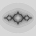
  p=3 rabbit
• 
  p=3 airplane
• 
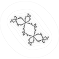
  p=4 rabbit
• 
  p=17

Description

Near super attracting fixed point (for example infinity) the behaviour of discrete dynamical system :

$z_{n+1}=f_{c}(z_{n})=z_{n}^{2}+c\,$

based on complex quadratic polynomial $f_{c}(z)=z^{2}+c\,$ is similar to

$w_{n+1}=f_{0}(w_{n})=w_{n}^{2}\,$

based on $f_{0}(w)=w^{2}\,$

It can be treated as one dynamical system viewed in two coordinate systems :

• easy ( w )
• hard to analyse( z )

In other words map $f_{c}\,$ is conjugate to map $f_{0}\,$ near infinity.

Names

• $w\,$ is Boettcher coordinate
• $\Phi _{c}\,$ is Boettcher function
• Boettcher Functional Equation:

 $\Phi _{c}(f_{c}(z))=\Phi _{c}(z)^{2}\,$

where :

 $w=\Phi _{c}(z)\,$

Complex potential or Boettcher coordinate has :

• radial values ( real potential ) LogPhi = CPM/J = value of the Green's function
• angular values ( external angle ) ArgPhi

Both values can be used to color with 2D gradient.

Computation

numerical solution

Methods

• Basic complex dynamicsA computational approach by Mark McClure see

Original approach

The Boettcher functional equation:

$F(f(z))=(F(z))^{m}$

where:

• f is a given function which is analytic in a neighborhood of its fixed point x
• F is the Boettcher's function

When the fixed point x is superattracting:

$f(z)=x+{\frac {(z-x)^{m}}{m!}}f^{m}(x)+{\frac {(z-x)^{m+1}}{(m+1)!}}f^{m+1}(x)+\ldots$

a “basic algorithm”:

$R(z)=\lim _{n\rightarrow \infty }{\sqrt[{m^{n}}]{fn(z)-z}}$

Let $\Xi (z)$ be a function such that

$\Xi (f(z))=\Xi (z)$

Then the general solution to the functional equation is given by:

$Q^{\Xi (z)(logR(z))}$

where Q is an arbitrary constant.

Mathemathica

Formula from Mathemathica

$w=B(c,z)=\lim _{n\to \infty }z_{n}^{\frac {1}{2^{n}}}\,$

To compute Boettcher coordinate $w\,$ use this formula

$w=\Phi _{c}(z)=z*\prod _{n=1}^{\infty }\left({\frac {f_{c}^{n}(z)}{f_{c}^{n}(z)-c}}\right)^{1/2^{n}}\,$

It looks "simple", but :

• square root of complex number gives two values so one have to choose one value
• more precision is needed near Julia set

PDE's approach

To construct a Riemann map explicitly on a given domain $D$ use the following PDE's approach

• first, translate the domain so that it contains the origin
• next, use a numerical method to construct a harmonic function $F$ satisfying $F(z)\;=\;-\log |z|$ for all $z\in \partial D$ , and let $R(z)=|z|e^{F(z)}.$

Then $R(0)=0$, $R|_{\partial D}\equiv 1$, and $\log R$ is harmonic, so $R$ is the radial component (i.e. modulus) of a Riemann map on $D$.

The angular component can now be determined by the fact that its level curves are perpendicular to the level curves of $R$, and have equal angular spacing near the origin.

Examples

The Basilica Julia set

• $c=-1$ is a center of period 2 hyperbolic component of Mandelbrot set
• fixed point $z=\alpha _{c}\,$
• superattracting 2-point cycle (limit cycle) :$\left\{z_{0}=0,z_{1}=f_{c}(z_{0})=c=-1\right\}\,$ ( period is 2 )
• 2 external rays : ${\mathcal {R}}_{\frac {1}{3}},{\mathcal {R}}_{\frac {2}{3}}$ which land on fixed point $z=\alpha _{c}\,$, which is a root point of the component of filled Julia set with center z=-1
• The pinch points for the Basilica are points have external rays at angles that are rational numbers of the form ${\frac {3k-1}{3*2^{n}}}$ and ${\frac {3k+1}{3*2^{n}}}$ for some k,n∈Nk, n ∈ Nk,n∈N.

Central component

Basilica lamination

Description

• the central bounded Fatou component
• large central component, which contains the origin of the complex plane
• it is a quotient of the central gap in the Basilica lamination, i.e. the gap containing the center point of the disk
• "It is obtained from the central gap by collapsing each of the infinitely many central arcs that surround this gap. We can label these central arcs using the dyadic rationals. Each central arc corresponds to a single point in the boundary ∂C of C the central component. These points are dense in ∂C, the labeling of the central arcs by dyadics induces a well-defined homeomorphism from ∂C to the unit circle"

Points:

• alpha fixed point and it's preimages

Boettchers equation

$f(z)=z^{2}-1$

Maxima CAS src code :

(%i1) kill(all);
(%o0)                                done
(%i1) remvalue(all);
(%o1)                                 []
(%i2) display2d:false;

(%o2) false
(%i3) define(f(z), z^2-1);

(%o3) f(z):=z^2-1
(%i4) a:factor(f(f(z)));

(%o4) z^2*(z^2-2)
(%i5) 
 taylor(a,z,0,14);

(%o5) (-2*z^2)+z^4

It gives Böttcher's functional equation:

${\mathcal {B}}(h(z))=g({\mathcal {B}}(z))$
 
${\mathcal {B}}(z^{4}-2*z^{2})=({\mathcal {B}}(z))^{2}$

Solve above functional equation for the Boettcher map ${\mathcal {B}}(z)$

The Riemann map for the central component for the Basilica

methods by James M. Belk for:

• drawing external rays
• Riemann map on the central component of Basilica

Description

• choose starting points with known Bottcher coordinates: the dyadic points on the boundary of central component
• compute a very large number of inverse images of these points
• draw curves through the right sequences of points

Here is a summary of the procedure for drawing equipotentials for a quadratic Julia set:

• Start with a large number (say 3 * 2^13) of equally spaced sample points on a circle of large radius (say R = 2^16) centered at the origin. Note that this circle is basically an equipotential for the Julia set, since the radius is so large.
• Compute an equal number of points on the inverse image of this circle (which is again basically an equipotential whose radius is the square root of R). Note that each of the original points has two preimages, so it must be worked out in each case which preimage to use.
• Iterate step 2 to produce sample points on a large number (say 50) of equipotentials that converge to the Julia set.

If you want to draw the external rays, it works to draw a piecewise-linear path between corresponding points on different equipotentials. Of course, the resulting external rays will be straight between the sample points, but you can fix this by using more than one orbit of equipotentials.

The Riemann map for the central component for the Basilica was drawn in essentially the same way, except that instead of starting with points on a big circle, I started with sample points on a circle of small radius (e.g. 0.00001) around the origin.

The Bubble bath Julia set

the Bottcher map is well defined (up to a choice of which ray to map to the angle zero) by the theorem on the previous page pp. 42

For the Bubble bath Julia set  :

$f(z)={\frac {1-z^{2}}{z^{2}}}$ 

A commutative diagram ( the picture describing function composition):

${\begin{array}{lcl}&U&{\overset {h}{\longrightarrow }}&U&\\&{\mathcal {B}}\downarrow &&\downarrow {\mathcal {B}}\\&D^{2}&{\underset {g}{\longrightarrow }}&D^{2}&\\\end{array}}$

Here:

• $U$ is the middle bubble ( component), whose center is z=0
• $D^{2}$ is the open unit disc, whose center is w=0
• $g$ is the function which maps unit disk to itself $g:D^{2}\to D^{2}$ and it's equation is $g(z)=z^{4}$
• $h$ is the function which maps middle bubble to itself $h:U\to U$ and it's equation is $h(z)=f^{3}(z)={\frac {z^{4}(z^{4}-4z^{2}+2)}{(2z^{2}-1)^{2}}}\approx 2z^{4}+4z^{6}+9z^{8}+20z^{10}+44z^{12}+96z^{14}$
• ${\mathcal {B}}$ is the Boettcher map which maps middle buble to unit disk ${\mathcal {B}}:U\to D^{2}$

Maxima CAS code

a:factor(f(f(f(z))));

(%o10)(z^4*(z^4-4*z^2+2))/(2*z^2-1)^2

 taylor(a,z,0,14);

(%o11) 2*z^4+4*z^6+9*z^8+20*z^10+44*z^12+96*z^14

In the above square diagram, commutativity of the diagram means:

${\mathcal {B}}\circ h=g\circ {\mathcal {B}}$.

It gives Böttcher's functional equation:

${\mathcal {B}}(h(z))=g({\mathcal {B}}(z))$
 
${\mathcal {B}}(2z^{4}+4z^{6}+9z^{8}+20z^{10}+44z^{12}+96z^{14})=({\mathcal {B}}(z))^{4}$

Solve above functional equation for the Boettcher map ${\mathcal {B}}(z)$

explicit closed form solution

• power maps $z\to z^{d}$
• Chebyshev polynomials

c = -2

Polar coordinate system and $\Psi _{c}$ for $c=-2$.

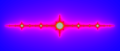
For c = -2 Julia set is a horizontal segment between -2 and 2 on the real axis:

$\ K_{-2}\ {\overset {\underset {\mathrm {def} }{}}{=}}\ \{z\in \mathbb {C} :-2\leq \operatorname {Re} (z)\leq 2,\operatorname {Im} (z)=0\}$

Now:

• equipotential lines are elipses
• field lines are hyperbolas
• Boettcher map and it's inverse have explicit equations ( closed-form expression ):

$\Phi _{-2}(z)={\frac {z+{\sqrt {z^{2}-4}}}{2}}\,$

$\Phi ^{-1}(w)=w+{\frac {1}{w}}\,$

where branch cut is taken to coincide with $\ K_{-2}$

See also:

• charged line segment
• Joukowsky transformation
• math.stackexchange question: explicitly-calculating-greens-function-in-complex-dynamics

History

In 1904 LE Boettcher:

• solved Schröder functional equation in case of supperattracting fixed point
• "proved the existence of an analytic function $\phi (z)\sim z$ near $\infty$ which conjugates the polynomial with $z^{d}$, that is $\phi \circ p(z)=\phi (z)^{d}$" ( Alexandre Eremenko )

LogPhi - Douady-Hubbard potential - real potential - radial component of complex potential

Aproximates distance to the fractal

• it is smooth
• it is 0 at the fractal and log|z| at infinity

The potential function and the real iteration number

The Julia set for $f(z)=z^{2}$ is the unit circle, and on the outer Fatou domain, the potential function φ(z) is defined by φ(z) = log|z|. The equipotential lines for this function are concentric circles. As $|f(z)|=|z|^{2}$ we have

$\varphi (z)=\lim _{k\to \infty }{\frac {\log |z_{k}|}{2^{k}}},$

where $z_{k}$ is the sequence of iteration generated by z. For the more general iteration $f(z)=z^{2}+c$, it has been proved that if the Julia set is connected (that is, if c belongs to the (usual) Mandelbrot set), then there exist a biholomorphic map ψ between the outer Fatou domain and the outer of the unit circle such that $|\psi (f(z))|=|\psi (z)|^{2}$. This means that the potential function on the outer Fatou domain defined by this correspondence is given by:

$\varphi (z)=\lim _{k\to \infty }{\frac {\log |z_{k}|}{2^{k}}}.$

This formula has meaning also if the Julia set is not connected, so that we for all c can define the potential function on the Fatou domain containing ∞ by this formula. For a general rational function f(z) such that ∞ is a critical point and a fixed point, that is, such that the degree m of the numerator is at least two larger than the degree n of the denominator, we define the potential function on the Fatou domain containing ∞ by:

$\varphi (z)=\lim _{k\to \infty }{\frac {\log |z_{k}|}{d^{k}}},$

where d = m − n is the degree of the rational function.

If N is a very large number (e.g. 10¹⁰⁰), and if k is the first iteration number such that $|z_{k}|>N$, we have that

${\frac {\log |z_{k}|}{d^{k}}}={\frac {\log(N)}{d^{\nu (z)}}},$

for some real number $\nu (z)$, which should be regarded as the real iteration number, and we have that:

$\nu (z)=k-{\frac {\log(\log |z_{k}|/\log(N))}{\log(d)}},$

where the last number is in the interval [0, 1).

For iteration towards a finite attracting cycle of order r, we have that if z* is a point of the cycle, then $f(f(...f(z^{*})))=z^{*}$ (the r-fold composition), and the number

$\alpha ={\frac {1}{\left|(d(f(f(\cdots f(z))))/dz)_{z=z^{*}}\right|}}\qquad (>1)$

is the attraction of the cycle. If w is a point very near z* and w' is w iterated r times, we have that

$\alpha =\lim _{k\to \infty }{\frac {|w-z^{*}|}{|w'-z^{*}|}}.$

Therefore the number $|z_{kr}-z^{*}|\alpha ^{k}$ is almost independent of k. We define the potential function on the Fatou domain by:

$\varphi (z)=\lim _{k\to \infty }{\frac {1}{(|z_{kr}-z^{*}|\alpha ^{k})}}.$

If ε is a very small number and k is the first iteration number such that $|z_{k}-z^{*}|<\epsilon$, we have that

$\varphi (z)={\frac {1}{(\varepsilon \alpha ^{\nu (z)})}}$

for some real number $\nu (z)$, which should be regarded as the real iteration number, and we have that:

$\nu (z)=k-{\frac {\log(\varepsilon /|z_{k}-z^{*}|)}{\log(\alpha )}}.$

If the attraction is ∞, meaning that the cycle is super-attracting, meaning again that one of the points of the cycle is a critical point, we must replace α by

$\alpha =\lim _{k\to \infty }{\frac {\log |w'-z^{*}|}{\log |w-z^{*}|}},$

where w' is w iterated r times and the formula for φ(z) by:

$\varphi (z)=\lim _{k\to \infty }{\frac {\log(1/|z_{kr}-z^{*}|)}{\alpha ^{k}}}.$

And now the real iteration number is given by:

$\nu (z)=k-{\frac {\log(\log |z_{k}-z^{*}|/\log(\varepsilon ))}{\log(\alpha )}}.$

For the colouring we must have a cyclic scale of colours (constructed mathematically, for instance) and containing H colours numbered from 0 to H−1 (H = 500, for instance). We multiply the real number $\nu (z)$ by a fixed real number determining the density of the colours in the picture, and take the integral part of this number modulo H.

The definition of the potential function and our way of colouring presuppose that the cycle is attracting, that is, not neutral. If the cycle is neutral, we cannot colour the Fatou domain in a natural way. As the terminus of the iteration is a revolving movement, we can, for instance, colour by the minimum distance from the cycle left fixed by the iteration.

CPM/J

Potential of filled Julia set

Diagram of potential computed with 2 methods : simple and full

Note that potential inside Kc is zero so :

Pseudocode version :

if (LastIteration==IterationMax)
 then potential=0    /* inside  Filled-in Julia set */
 else potential= GiveLogPhi(z0,c,ER,nMax); /* outside */

It also removes potential error for log(0).

Full version

Math (full) notation :

$LogPhi_{c}(z)=ln|z|+\sum _{n=1}^{\infty }{\frac {1}{2^{n}}}ln|1+{\frac {c}{(f_{c}^{n-1}(z))^{2}}}|$

Maxima (full) function :

GiveLogPhi(z0,c,ER,nMax):=
block(
 [z:z0,
 logphi:log(cabs(z)),
 fac:1/2,
 n:0],
 while n<nMax and abs(z)<ER do
 (z:z*z+c,
 logphi:logphi+fac*log(cabs(1+c/(z*z))),
 n:n+1
 ),
 return(float(logphi))
)$

Simplified version

The escape rate function of a polynomial f is defined by :

$G_{f}(z)=\lim _{n\rightarrow \infty }{\frac {1}{2^{n}}}log^{+}|f^{n}(z)|\,$

where :

$log^{+}=max(log,0)$

"The function Gp is continous on C and harmonic on the complement of the Julia set. It vanishes identically on K(f) and as it has a logarithmic pole at infinity, it is a it is the Green's function for C/ K(f)." ( Laura G. DeMarco)

Math simplified formula :

$SLogPhi_{c}(z)={\frac {log(f^{n}(z))}{2^{n}}}\,$

Maxima function :

GiveSLogPhi(z0,c,e_r,i_max):=
 block(
  [z:z0,
   logphi,
   fac:1/2,
   i:0
  ],
  while i<i_max and cabs(z)<e_r do
  (z:z*z+c,
    fac:fac/2,
    i:i+1
  ),
 logphi:fac*log(cabs(z)),
 return(float(logphi))
)$

If you don't check if orbit is not bounded ( escapes, bailout test) then use this Maxima function :

GiveSLogPhi(z0,c,e_r,i_max):=
block(
 [z:z0, logphi, fac:1/2, i:0],
  while i<i_max and cabs(z)<e_r do
   (z:z*z+c,
    fac:fac/2,
    i:i+1 ),
   if i=i_max
    then logphi:0
    else logphi:fac*log(cabs(z)),
   float(logphi) 
)$

C version :

double jlogphi(double zx0, double zy0, double cx, double cy)
/* this function is based on function by W Jung http://mndynamics.com */
{ 
 int j; 
 double 
 zx=zx0,
 zy=zy0,
 s = 0.5, 
 zx2=zx*zx,
 zy2=zy*zy,
 t;
 for (j = 1; j < 400; j++)
 { s *= 0.5; 
  zy = 2 * zx * zy + cy;
  zx = zx2 - zy2 + cx; 
  zx2 = zx*zx; 
  zy2 = zy*zy;
  t = fabs(zx2 + zy2); // abs(z)
  if ( t > 1e24) break; 
 } 
return s*log2(t);  // log(zn)* 2^(-n)
}//jlogphi

Euler version by R. Grothmann ( with small change : from z^2-c to z^2+c) :

function iter (z,c,n=100) ...

h=z;
loop 1 to n;
h=h^2+c;
if totalmax(abs(h))>1e20; m=#; break; endif;
end;
return {h,m};
endfunction

x=-2:0.05:2; y=x'; z=x+I*y;
{w,n}=iter(z,c);
wr=max(0,log(abs(w)))/2^n;

Level Sets of potential = pLSM/J

Here is Delphi function which gives level of potential :

Function GiveLevelOfPotential(potential:extended):integer;
 var r:extended;
 begin
    r:= log2(abs(potential));
    result:=ceil(r);
 end;

Level Curves of potential = equipotential lines = pLCM/J

The continuous potential formula doesn't align properly with iteration bands

ArgPhi - External angle (angular component of complex potential) and external ray

One can start with binary decomposition of basin of attraction of infinity.

The second step can be using $\Psi _{c}\,$

period of angle under doubling map

How to find period of external angle measured in turns under doubling map :

Here is Common Lisp code :

(defun give-period (ratio-angle)
  "gives period of angle in turns (ratio) under doubling map"
  (let* ((n (numerator ratio-angle))
	 (d (denominator ratio-angle))
	 (temp n)) ; temporary numerator
    
    (loop for p from 1 to 100 do 
	  (setq temp  (mod (* temp 2) d)) ; (2 x n) modulo d = doubling)
	  when ( or (= temp n) (= temp 0)) return p )))

Maxima CAS code :

doubling_map(n,d):=mod(2*n,d);

/* catch-throw version by Stavros Macrakis, works */
GivePeriodOfAngle(n0,d):=
catch(
      block([ni:n0],
          for i thru 200 do if (ni:doubling_map(ni,d))=n0 then throw(i),
          0 ) )$

/* go-loop version, works */
GiveP(n0,d):=block(
[ni:n0,i:0],
block(
  loop,
  ni:doubling_map(ni,d),
  i:i+1,
  if i<100 and not (n0=ni) then go(loop)
),
if (n0=ni) 
	then i 
	else 0
);

/* Barton Willis while version without for loop , works */
GivePeriod(n0,d):=block([ni : n0,k : 1],
  while (ni : doubling_map(ni,d)) # n0 and k < 100 do (
    k : k + 1),
  if k = 100 then 0 else k)$

Computing external angle

External angle (argument) is argument of Boettcher coordinate $w\,$

$arg_{c}(z)=arg(w)=arg(\Phi _{c}(z))\,$

Because Boettcher coordinate is a product of complex numbers

$w=\Phi _{c}(z)=z*\prod _{n=1}^{\infty }\left({\frac {f_{c}^{n}(z)}{f_{c}^{n}(z)-c}}\right)^{1/2^{n}}\,$

so argument of product is :

$arg_{c}(z)=arg(z)+\sum _{n=1}^{\infty }\left({\frac {1}{2^{n}}}*arg\left({\frac {f_{c}^{n}(z)}{f_{c}^{n}(z)-c}}\right)\right)\,$

dynamic external rays

Dynamic external rays description

Lamination of dynamical plane

Lamination of rabbit Julia set

Here is long description

See also

• complex potential on parameter plane
• precision - how important it is

References

• Ricardo A. Oliva: On the Combinatorics of External Rays in the Dynamics of the Complex Henon Map.
• A Thompson-Like Group for the Bubble Bath Julia Set by Jasper Weinrich-Burd Boettcher map and internal rays
• Fixed curves near fixed points by Alastair Fletcher
• Mandelson set area via the Böttcher series by Geoffrey Irving and colab doc description