Fractals/Computer graphic techniques/2D/algorithms

Algorithms

postprocessing = modification of the image = graphic algorithms = image processing

Algorithms by graphic type

• raster algorithms
• vector algorithms

Five classes of image processing algorithms:

• image restoration
• image analysis
• image synthesis
• image enhancement
• image compression.

List:

• Color Theory: Color gradient
• 2D Plane transformations
  • 2D to 3D
    • heightmaps
    • slope

• Morphological operations on binary images
  • morphological closing = dilation followed by erosion
  • morphological opening = erosion followed by dilation

Postprocessing

• Two types of edge detection
• Pseudo-3D projections
• Star field generator
• Random dot stereograms (aka Magic Eye)
• Motion blur for animations
• Interlacing
• Embossing
• Antialiasing
• Palette emulation to allow color cycling on true-color displays
• True color emulation that provides dithering on 256-color display

Algorithms:

• coloring after and independently of the fractal creation using gradient maps
  • histogram colorings
• gamma correction of dense images
• Histogram equalization in wikipedia
• (matrix) convolution ( = discrete convolution) is an element-wise multiplication of two matrices followed by a sum
  • image convolution
    • LIC

types

range

The image processing operators ( algorithms) can be classified into the 4 categories

• pixel algorithms = pixel processing: the point operator acts on individual pixels : g = H(f)
  • add two images: g(x)=f1(x)+f2(x)
  • the histogram
  • look-up table (LUT)
  • windowing
• local algorithms = kernaling = local processing: "A local operator calculates the pixel value g(x) based not only on the value in the same position in the input image, i.e. f(x) , but it used several values in nearby points f(x+y). Local operators are at the heart of almost all image processing tasks."
  • spatial location filtering (convolution),
  • spatial frequency filtering using high- and low-pass digital filters,
  • the unsharp masking technique
• geometric processing = geometric transformations: "Whereas a point operator changes the value of all pixels a geometrical operator doesn’t change the value but instead it ‘moves’ a pixel to a new position."
• Global Operators: "A global operator (potentially) needs al pixel values in the input image to calculate the value for just one pixel in the output image."

Libraries

• DGtal = Digital Geometry Tools and Algorithms Library in C++
• CGAL - The Computational Geometry Algorithms Library in C++
• Habrador - Computational-geometry in C#
• Manipulation and analysis of geometric objects in Python

Digital topology

• HIPR --- The Hypermedia Image Processing Reference by R. Fisher, S. Perkins, A. Walker and E. Wolfart.
• Topological tools for discrete shape analysis by John Chaussard

geometry

• hyperbolic
  • hyperbolic

light

• image-based-lighting by Mikael Hvidtfeldt Christensen
• Global Illumination Compendium September 29, 2003 by Philip Dutré

• 
  Light sources

gamma correction

• gamma-correction by Mikael Hvidtfeldt Christensen

dense image

Dense image

• downscaling with gamma correction
• path finding
• aliasing
• changing algorithm ( representation function) from discrete to continous, like from level set method of escape time to continous ( DEM )

  "the denser the area, the more heavy the anti-aliasing have to be in order to make it look good."  knighty

  "the details are smaller than pixel spacing, so all that remains is the bands of colour shift from period-doubling of features making it even denser"  claude

tiling

• tiling editor
• Tiling Bot by Roice Nelson
• draw the Wythoff construction of uniform tilings in hyperbolic plane
• EPINET = Euclidean Patterns In Non-Euclidean Tilings

path finding

path finding

• old fractal forums : pathfinding-in-the-mandelbrot-set/
• fractalforums.org : pathfinding-in-the-mandelbrot-set-revisited
• 5-ways-to-find-the-shortest-path-in-a-graph by Johannes Baum
• mathreference - graph

Algorithms

• Depth-First Search (DFS) = the simplest algorithm
• Breadth-First Search (BFS)
• Bidirectional Search
• Dijkstra's algorithm (or Dijkstra's Shortest Path First algorithm, SPF algorithm)
  • programiz : dijkstra-algorithm
  • dyclassroom : dijkstra-algorithm-finding-shortest-path
• Bellman-Ford Algorithm

size

• how to opern big image
  • vliv: The principle behind Vliv (only load parts of the image that is visible, and leverage the TIFF format - tiled pyramidal images) can be implemented on any OS. The API for plugins consists only of 5 functions, see the vlivplugins repo for examples.

resizing

Methods:

• Image Magic resize
• FF
• 2^x Image Super-Resolution
  • Final2x
  • image-super-resolution

polygons

• geometric operations for two-dimensional polygons

How to tell whether a point is to the right or left side of a line ?

/* 
  How to tell whether a point is to the right or left side of a line ?

 http://stackoverflow.com/questions/1560492/how-to-tell-whether-a-point-is-to-the-right-or-left-side-of-a-line

  a, b = points
  line = ab
 pont to check = z

  position = sign((Bx - Ax) * (Y - Ay) - (By - Ay) * (X - Ax))
  It is 0 on the line, and +1 on one side, -1 on the other side.

*/

double CheckSide(double Zx, double Zy, double Ax, double Ay, double Bx, double By)
{
  return ((Bx - Ax) * (Zy - Ay) - (By - Ay) * (Zx - Ax));

}

Testing if point is inside triangle

• description
• javascript code

/* 
c console program 
gcc t.c -Wall
./a.out

*/

# include <stdio.h>

// 3 points define triangle 
double Zax = -0.250000000000000;
double Zay = 0.433012701892219;
// left when y
double Zlx = -0.112538773749444;  
double Zly = 0.436719687479814 ;

double Zrx = -0.335875821657728;
double Zry = 0.316782798339332;

// points to test 
// = inside triangle 
double Zx = -0.209881783739630;
double Zy =   +0.4;

// outside triangle 
double Zxo = -0.193503885412548  ;
double Zyo = 0.521747636163664;

double Zxo2 = -0.338750000000000;
double Zyo2 = +0.440690927838329;

// ============ http://stackoverflow.com/questions/2049582/how-to-determine-a-point-in-a-2d-triangle
// In general, the simplest (and quite optimal) algorithm is checking on which side of the half-plane created by the edges the point is.
double sign (double  x1, double y1,  double x2, double y2, double x3, double y3)
{
    return (x1 - x3) * (y2 - y3) - (x2 - x3) * (y1 - y3);
}

int  PointInTriangle (double x, double y, double x1, double y1, double x2, double y2, double x3, double y3)
{
    double  b1, b2, b3;

    b1 = sign(x, y, x1, y1, x2, y2) < 0.0;
    b2 = sign(x, y, x2, y2, x3, y3) < 0.0;
    b3 = sign(x, y, x3, y3, x1, y1) < 0.0;

    return ((b1 == b2) && (b2 == b3));
}

int Describe_Position(double Zx, double Zy){
if (PointInTriangle( Zx, Zy, Zax, Zay, Zlx, Zly, Zrx, Zry))
  printf(" Z is inside \n");
  else printf(" Z is outside \n");

return 0;
}

// ======================================

int main(void){

Describe_Position(Zx, Zy);
Describe_Position(Zxo, Zyo);
Describe_Position(Zxo2, Zyo2);

return 0;
}

Orientation and area of the triangle

Orientation and area of the triangle : how to do it ?

// gcc t.c -Wall
// ./a.out
# include <stdio.h>

// http://ncalculators.com/geometry/triangle-area-by-3-points.htm
double GiveTriangleArea(double xa, double ya, double xb, double yb, double xc, double yc)
{
return ((xb*ya-xa*yb)+(xc*yb-xb*yc)+(xa*yc-xc*ya))/2.0;
}

/*

wiki Curve_orientation
[http://mathoverflow.net/questions/44096/detecting-whether-directed-cycle-is-clockwise-or-counterclockwise]

The orientation of a triangle (clockwise/counterclockwise) is the sign of the determinant

matrix = { {1 , x1, y1}, {1 ,x2, y2} , {1,  x3, y3}}

where 
(x_1,y_1), (x_2,y_2), (x_3,y_3)$ 
are the Cartesian coordinates of the three vertices of the triangle.

:<math>\mathbf{O} = \begin{bmatrix}

1 & x_{A} & y_{A} \\
1 & x_{B} & y_{B} \\
1 & x_{C} & y_{C}\end{bmatrix}.</math>

A formula for its determinant may be obtained, e.g., using the method of [[cofactor expansion]]:
:<math>\begin{align}
\det(O) &= 1\begin{vmatrix}x_{B}&y_{B}\\x_{C}&y_{C}\end{vmatrix}
-x_{A}\begin{vmatrix}1&y_{B}\\1&y_{C}\end{vmatrix}
+y_{A}\begin{vmatrix}1&x_{B}\\1&x_{C}\end{vmatrix} \\
&= x_{B}y_{C}-y_{B}x_{C}-x_{A}y_{C}+x_{A}y_{B}+y_{A}x_{C}-y_{A}x_{B} \\
&= (x_{B}y_{C}+x_{A}y_{B}+y_{A}x_{C})-(y_{A}x_{B}+y_{B}x_{C}+x_{A}y_{C}).
\end{align}
</math>

If the determinant is negative, then the polygon is oriented clockwise.  If the determinant is positive, the polygon is oriented counterclockwise.  The determinant  is non-zero if points A, B, and C are non-[[collinear]].  In the above example, with points ordered A, B, C, etc., the determinant is negative, and therefore the polygon is clockwise.

*/

double IsTriangleCounterclockwise(double xa, double ya, double xb, double yb, double xc, double yc)
{return  ((xb*yc + xa*yb +ya*xc) - (ya*xb +yb*xc + xa*yc)); }

int DescribeTriangle(double xa, double ya, double xb, double yb, double xc, double yc)
{
 double t = IsTriangleCounterclockwise( xa,  ya, xb,  yb,  xc,  yc);
 double a = GiveTriangleArea( xa,  ya, xb,  yb,  xc,  yc);
 if (t>0)  printf("this triangle is oriented counterclockwise,     determinent = %f ; area = %f\n", t,a);
 if (t<0)  printf("this triangle is oriented clockwise,            determinent = %f; area = %f\n", t,a);
 if (t==0) printf("this triangle is degenerate: colinear or identical points, determinent = %f; area = %f\n", t,a);

 return 0;
}

int main()
{
 // clockwise oriented triangles 
 DescribeTriangle(-94,   0,  92,  68, 400, 180); // https://www-sop.inria.fr/prisme/fiches/Arithmetique/index.html.en
 DescribeTriangle(4.0, 1.0, 0.0, 9.0, 8.0, 3.0); // clockwise orientation https://people.sc.fsu.edu/~jburkardt/datasets/triangles/tex5.txt
 
 //  counterclockwise oriented triangles
 DescribeTriangle(-50.00, 0.00, 50.00,  0.00, 0.00,  0.02); // a "cap" triangle. This example has an area of 1.
 DescribeTriangle(0.0,  0.0, 3.0,  0.0, 0.0,  4.0); // a right triangle. This example has an area of (?? 3 ??)  =  6
 DescribeTriangle(4.0, 1.0, 8.0, 3.0, 0.0, 9.0);  //      https://people.sc.fsu.edu/~jburkardt/datasets/triangles/tex1.txt
 DescribeTriangle(-0.5, 0.0,  0.5,  0.0, 0.0,  0.866025403784439); // an equilateral triangle. This triangle has an area of sqrt(3)/4.

 // degenerate triangles 
 DescribeTriangle(1.0, 0.0, 2.0, 2.0, 3.0, 4.0); // This triangle is degenerate: 3 colinear points. https://people.sc.fsu.edu/~jburkardt/datasets/triangles/tex6.txt
 DescribeTriangle(4.0, 1.0, 0.0, 9.0, 4.0, 1.0); //2 identical points 
 DescribeTriangle(2.0, 3.0, 2.0, 3.0, 2.0, 3.0); // 3 identical points

 return 0; 
}

Testing if point is inside polygon

• stackoverflow
• description by W Muła
• point_in_polygon by Patrick Glauner
  • A Simple and Correct Even-Odd Algorithm for the Point-in-Polygon Problem for Complex Polygons by Michael Galetzka, Patrick O. Glauner
  • c code
• PNPOLY - Point Inclusion in Polygon Test - W. Randolph Franklin (WRF)

Point_in_polygon_problem : image and source code

/*

gcc p.c -Wall
./a.out

----------- git --------------------
cd existing_folder
git init
git remote add origin git@gitlab.com:adammajewski/PointInPolygonTest_c.git
git add .
git commit
git push -u origin master

*/

#include <stdio.h>

#define LENGTH 6

/*

Argument	Meaning
nvert	Number of vertices in the polygon. Whether to repeat the first vertex at the end is discussed below.
vertx, verty	Arrays containing the x- and y-coordinates of the polygon's vertices.
testx, testy	X- and y-coordinate of the test point.

https://www.ecse.rpi.edu/Homepages/wrf/Research/Short_Notes/pnpoly.html
PNPOLY - Point Inclusion in Polygon Test
W. Randolph Franklin (WRF)

	

I run a semi-infinite ray horizontally (increasing x, fixed y) out from the test point, 
and count how many edges it crosses. 
At each crossing, the ray switches between inside and outside. 
This is called the Jordan curve theorem.
The case of the ray going thru a vertex is handled correctly via a careful selection of inequalities. 
Don't mess with this code unless you're familiar with the idea of Simulation of Simplicity. 
This pretends to shift the ray infinitesimally down so that it either clearly intersects, or clearly doesn't touch. 
Since this is merely a conceptual, infinitesimal, shift, it never creates an intersection that didn't exist before, 
and never destroys an intersection that clearly existed before.

The ray is tested against each edge thus:

Is the point in the half-plane to the left of the extended edge? and
Is the point's Y coordinate within the edge's Y-range?
Handling endpoints here is tricky.

I run a semi-infinite ray horizontally (increasing x, fixed y) out from the test point, 
and count how many edges it crosses. At each crossing, 
the ray switches between inside and outside. This is called the Jordan curve theorem.
The variable c is switching from 0 to 1 and 1 to 0 each time the horizontal ray crosses any edge. 
So basically it's keeping track of whether the number of edges crossed are even or odd. 
0 means even and 1 means odd.

*/

int pnpoly(int nvert, double *vertx, double *verty, double testx, double testy)
{
  int i, j, c = 0;
  for (i = 0, j = nvert-1; i < nvert; j = i++) {
    if ( ((verty[i]>testy) != (verty[j]>testy)) &&
	 (testx < (vertx[j]-vertx[i]) * (testy-verty[i]) / (verty[j]-verty[i]) + vertx[i]) )
       c = !c;
  }

  return c;
}

void CheckPoint(int nvert, double *vertx, double *verty, double testx, double testy){

int flag;

flag =  pnpoly(nvert, vertx, verty, testx, testy);

 switch(flag){
   case 0  : printf("outside\n"); break;
   case 1  : printf("inside\n"); break;
   default : printf(" ??? \n");
 }
}

int main (){

// values from http://stackoverflow.com/questions/217578/how-can-i-determine-whether-a-2d-point-is-within-a-polygon
// number from 0 to (LENGTH-1)
double zzx[LENGTH] = { 13.5,  6.0, 13.5, 42.5, 39.5, 42.5};
double zzy[LENGTH] = {100.0, 70.5, 41.5, 56.5, 69.5, 84.5};

CheckPoint(LENGTH, zzx, zzy, zzx[4]-0.001, zzy[4]);
CheckPoint(LENGTH, zzx, zzy, zzx[4]+0.001, zzy[4]);

return 0;
}

curve

types:

• closed/open
• with/without multiple points

methods

• tracing /drawing : Generating Discrete Curves
• sketching
• sampling
• Pathfinding or pathing is the plotting, by a computer application, of the shortest route between two points
• clipping
• Approximation of digitized curves (with cubic Bézier splines )
• curve fitting
• Mending broken lines
• edge detection

Examples

• line
  • bresenhams-drawing-algorithms
  • antyaliasing

• circle

Morton codes

• libmorton C++ header-only library with methods to efficiently encode/decode Morton codes in/from 2D/3D coordinates
• aavenel mortonlib

morphing

• Interpolations from a circle to a triangle in p5.js by Golan Levin

curve simplifying

reduce the number of points, but still keep the overall shape of the curve = PolyLine Reduction

• Ramer–Douglas–Peucker_algorithm
  • JS interactive maps library by Vladimir Agafonkin, It uses a combination of Douglas-Peucker and Radial Distance algorithms.
• Visvalingam–Whyatt algorithm
  • Permafacture: Py-Visvalingam-Whyatt ( Python code)

curve fitting

• my curve fit: online curve fitting

thick line drawing

thick line

• The Beauty of Bresenham's Algorithm by Alois Zingl
• Murphy's Modified Bresenham Line Drawing Algorithm
• stackoverflow question: how-do-i-create-a-line-of-arbitrary-thickness-using-bresenham

curve drawing

• Curve-Drawing Algorithms for Raster Displays by JERRY VAN AKEN and MARK NOVAK
• A Rasterizing Algorithm for Drawing Curves by Alois Zingl Wien, 2012
• Curve-Drawing Algorithms for Raster Displays by JERRY VAN AKEN and MARK NOVAK
• A* Pathfinding for Beginners By Patrick Lester (Updated July 18, 2005)
• Max K. Agoston Computer Graphics and Geometric Modeling Implementation and Algorithms
• libspiro is the creation of Raph Levien. It simplifies the drawing of beautiful curves
• spiro An interpolating spline based on spirals

neighborhood variants of 2D algorithms:

• 8-way stepping (8WS) for 8-direction neighbors of a pixel p(x, y)
• 4-way stepping (4WS) 4-direction neighbors of a pixel p(x, y)

• 2D neighborhood
• 
  4
• 
  8

curve sampling

• uniform = gives equidistant points
• adaptive. " an adaptive method for sampling the domain with respect to local curvature. Samples concentration is in proportion to this curvature, resulting in a more efficient approximation—in the limit, a flat curve is approximated by merely two endpoints."

• ocaml-curve-sampling by Christophe Troestler
• xahlee : adaptive_sampling_plot_math_curve

Field lines

Field line

• Vector fied : Field line computing
• external rays
  • parameter
  • dynamic
• gravitational field lines by Chris Thomasson. Images and AS3 code

Tracing

Tracing a curve on a triangular grid

Tracing curve

Methods

• general, (analytic or systematic) = curve sketching
• local method

Task: draw a 2D curve when

• there is no equaation of the line
• there are all the numerical values for the line within a certain range

trace an external ray for angle t in turns, which means ( description by Claude Heiland-Allen)

• starting at a large circle (e.g. r = 65536, x = r cos(2 pi t), y = r sin(2 pi t))
• following the escape lines (like the edges of binary decomposition colouring with large escape radius) in towards the Mandelbrot set.

this algorithm is O(period^2), which means doubling the period takes 4x as long, so it's only really feasible for periods up to a few 1000.

Three Curve Tracing Models

• Pixel-by-Pixel tracing
• brute force: If your line is short enough (less than 10^6 points), you can do this by calculating the distance from point p to each point in your discretized line, and take the minimum of these distances.
• The bipartite receptive field operator
• The zoom lens operator

Images

• Images in category Curve tracing from commons

Problems:

• intersection and Breadth-first search

Examples

• Numerical Methods for Particle Tracing in Vector Fields by Kenneth I. Joy

Curve rasterisation

Ray

Ray can be parametrised with radius (r)

Closed curve

Simple closed curve ("a connected curve that does not cross itself and ends at the same point where it begins" = having no endpoints) can be parametrized with angle (t).

Border, boundary, contour, edge

• Filling contour
• Finds contours in a binary image
• CavalierContoursWebDemo aand code

contour models

• snakes = active contour models

border tracing

• Contour tracing algorithms by Abeer George Ghuneim
• Tracing Boundaries in 2D Images by V. Kovalevsky
• wikipedia : Boundary tracing
• Calculating contour curves for 2D scalar fields
  • the marching squares algorithm for tracing contour curves on a scalar 2D field
• Smooth Contours
• contour polygons
• boundary in C++ by Shawn Halayka - 2019 and new code
• opencv_contour in C++ by Shawn Halayka
• CONREC A Contouring Subroutine Written by Paul Bourke July 1987 ( using triangulation)

Filling contour

• 
  Filling contour - simple procedure in c

Edge detection

• Boundary scanning method for Julia set - BSM/J
• Boundary scanning method for Mandelbrot set - BSM/M
• edge detection in Matlab
• Marching squares algorithm to generate contour lines
• The Roberts cross operator is used in image processing and computer vision for edge detection.

• 
  Level curves - edge detection (2 filters)
• 
  Edge detection of boundaries of level sets of escape time

Sobel filter

Short introduction

Sobel filter G consist of 2 kernels (masks):

• Gh for horizontal changes.
• Gv for vertical changes.

Sobel kernels

8-point neighborhood on a 2D grid

2D Convolution Animation

The Sobel kernel contains weights for each pixel from the 8-point neighbourhood of a tested pixel. These are 3x3 kernels.

There are 2 Sobel kernels, one for computing horizontal changes and other for computing vertical changes. Notice that a large horizontal change may indicate a vertical border, and a large vertical change may indicate a horizontal border. The x-coordinate is here defined as increasing in the "right"-direction, and the y-coordinate is defined as increasing in the "down"-direction.

The Sobel kernel for computing horizontal changes is:

$\mathbf {H} ={\begin{bmatrix}H_{1}&H_{2}&H_{3}\\H_{4}&H_{5}&H_{6}\\H_{7}&H_{8}&H_{9}\end{bmatrix}}={\begin{bmatrix}-1&0&+1\\-2&0&+2\\-1&0&+1\end{bmatrix}}$

The Sobel kernel for computing vertical changes is:

$\mathbf {V} ={\begin{bmatrix}-1&-2&-1\\\ \ 0&\ \ 0&\ \ 0\\+1&+2&+1\end{bmatrix}}$

Note that:

• sum of weights of kernels are zero

$\sum _{i=1}^{9}H_{i}=0$

$\sum _{i=1}^{9}V_{i}=0$

• One kernel is simply the other rotated by 90 degrees.
• 3 weights in each kernal are zero.

Pixel kernel

Pixel kernel A containing central pixel $A_{5}$ with its 3x3 neighbourhood:

$\mathbf {A} ={\begin{bmatrix}A_{1}&A_{2}&A_{3}\\A_{4}&A_{5}&A_{6}\\A_{7}&A_{8}&A_{9}\end{bmatrix}}$

Other notations for pixel kernel:

$\mathbf {A} ={\begin{bmatrix}A_{1}&A_{2}&A_{3}\\A_{4}&A_{5}&A_{6}\\A_{7}&A_{8}&A_{9}\end{bmatrix}}={\begin{bmatrix}ul&um&ur\\ml&mm&mr\\ll&lm&lr\end{bmatrix}}$

where:

unsigned char ul, // upper left
unsigned char um, // upper middle
unsigned char ur, // upper right
unsigned char ml, // middle left
unsigned char mm, // middle = central pixel
unsigned char mr, // middle right
unsigned char ll, // lower left
unsigned char lm, // lower middle
unsigned char lr, // lower right

Pixel 3x3 neighbourhood (with Y axis directed down)

In array notation it is:

$\mathbf {A} ={\begin{bmatrix}A[x-1][y+1]&A[x][y+1]&A[x+1][y+1]\\A[x-1][y]&A[x][y]&A[x+1][y]\\A[x-1][y-1]&A[x][y-1]&A[x+1][y-1]\end{bmatrix}}$

In geographic notation usede in cellular aotomats it is central pixel of Moore neighbourhood.

So central (tested) pixel is:

$A_{5}=mm=A[x][y]\,$

Sobel filters

Compute Sobel filters (where $*$ here denotes the 2-dimensional convolution operation not matrix multiplication). It is a sum of products of pixel and its weights:

$\mathbf {G} _{h}=\mathbf {H} *A=A_{1}H_{1}+A_{2}H_{2}+\cdots +A_{9}H_{9}=\sum _{r=1}^{9}A_{r}H_{r},$

$\mathbf {G} _{v}=\mathbf {V} *A=A_{1}V_{1}+A_{2}V_{2}+\cdots +A_{9}V_{9}=\sum _{r=1}^{9}A_{r}V_{r},$

Because 3 weights in each kernal are zero so there are only 6 products.

short Gh = ur + 2*mr + lr - ul - 2*ml - ll;
short Gv = ul + 2*um + ur - ll - 2*lm - lr;

Result

Result is computed (magnitude of gradient):

$\mathbf {G} (A_{5})={\sqrt {{\mathbf {G} _{h}}^{2}+{\mathbf {G} _{v}}^{2}}}$

It is a color of tested pixel.

One can also approximate result by sum of 2 magnitudes:

$\mathbf {G} (A_{5})=\left|\mathbf {G} _{h}\right|+\left|\mathbf {G} _{v}\right|$

which is much faster to compute.

Algorithm

• choose pixel and its 3x3 neighberhood A
• compute Sobel filter for horizontal Gh and vertical lines Gv
• compute Sobel filter G
• compute color of pixel

Programming

Sobel filters (2 filters 3x3): image and full c code

Skipped pixel - some points from its neighbourhood are out of the image

Lets take array of 8-bit colors (image) called data. To find borders in this image simply do:

for(iY=1;iY<iYmax-1;++iY){ 
    for(iX=1;iX<iXmax-1;++iX){ 
     Gv= - data[iY-1][iX-1] - 2*data[iY-1][iX] - data[iY-1][iX+1] + data[iY+1][iX-1] + 2*data[iY+1][iX] + data[iY+1][iX+1];
     Gh= - data[iY+1][iX-1] + data[iY-1][iX+1] - 2*data[iY][iX-1] + 2*data[iY][iX+1] - data[iY-1][iX-1] + data[iY+1][iX+1];
     G = sqrt(Gh*Gh + Gv*Gv);
     if (G==0) {edge[iY][iX]=255;} /* background */
         else {edge[iY][iX]=0;}  /* boundary */
    }
  }

Note that here points on borders of array (iY= 0, iY = iYmax, iX=0, iX=iXmax) are skipped

Result is saved to another array called edge (with the same size).

One can save edge array to file showing only borders, or merge 2 arrays:

for(iY=1;iY<iYmax-1;++iY){ 
    for(iX=1;iX<iXmax-1;++iX){ if (edge[iY][iX]==0) data[iY][iX]=0;}}

to have new image with marked borders.

Above example is for 8-bit or indexed color. For higher bit colors "the formula is applied to all three color channels separately" (from RoboRealm doc).

Other implementations:

• ImagMagic discussion: using a Sobel operator - edge detection
• Sobel in c from GIMP code
• Cpp code by Aaron Brooks - Brent Bolton - Jason O'Kane
• rosettacode: Image convolution
• C and opencl by royger
• C++ by Glenn Fiedler
• Convolution and Deconvolution
• Sobel Edge Detector by R. Fisher, S. Perkins, A. Walker and E. Wolfart with examples in Java
• Qt and GDI+ versions of the Sobel edge detection algorithm by Ken Earle
• Qt and OpenCV

Problems

Bad edge position seen in the middle of image. Lines are not meeting in good points, like z = 0

Edge position:

In ImageMagick as "you can see, the edge is added only to areas with a color gradient that is more than 50% white! I don't know if this is a bug or intentional, but it means that the edge in the above is located almost completely in the white parts of the original mask image. This fact can be extremely important when making use of the results of the "-edge" operator."

The result is:

• doubling edges; "if you are edge detecting an image containing an black outline, the "-edge" operator will 'twin' the black lines, producing a weird result."
• lines are not meeting in good points.

See also new operators from 6 version of ImageMagick: EdgeIn and EdgeOut from Morphology

Edge thickening

dilation

convert $tmp0 -convolve "1,1,1,1,1,1,1,1,1" -threshold 0 $outfile

SDF Signed Distance Function

• Vector_field SDF

test external tangency of 2 circles

/*
 distance between 2 points 
  z1 = x1 + y1*I
  z2 = x2 + y2*I
  en.wikipedia.org/wiki/Distance#Geometry
 
*/ 
 
double GiveDistance(int x1, int y1, int x2, int y2){
  return sqrt((x1-x2)*(x1-x2) + (y1-y2)*(y1-y2));
}

/*
mutually and externally tangent circles
mathworld.wolfram.com/TangentCircles.html
Two circles are mutually and externally tangent if distance between their centers is equal to the sum of their radii

*/

double TestTangency(int x1, int y1, int r1, int x2, int y2, int r2){
  double distance;

  distance = GiveDistance(x1, y1, x2, y2);
  return ( distance - (r1+r2));
// return should be zero
}

map projections

• Map projections in wikipedia
• Category:Map projections in commons
• commons Category:Map_projections_with_Tissot_s_indicatrix
• jkunimune Map-Projections

Stereographic

Stereographic projection is a map projection obtained by projecting points P on the surface of sphere from the sphere's north pole N to point P' in a plane tangent to the south pole S.

take the north pole N to be the standard unit vector (0, 0, 1) and the center of the sphere to be the origin, so that the tangent plane at the south pole is has equation z = 1. Given a point P = (x, y, z) on the unit sphere which is not the north pole, its image is equal to

$P'=f(P)=({\frac {2x}{1-z}},{\frac {2y}{1-z}})=(u,v)$

• 
• 
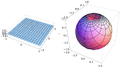  A Cartesian grid on the plane appears distorted on the sphere. The grid lines are still perpendicular, but the areas of the grid squares shrink as they approach the north pole.
• 
  A polar grid on the plane appears distorted on the sphere. The grid curves are still perpendicular, but the areas of the grid sectors shrink as they approach the north pole
• 

cylindrical

Cylindrical projections in general have an increased vertical stretching as one moves towards either of the poles. Indeed, the poles themselves can't be represented (except at infinity). This stretching is reduced in the  Mercator projection by the natural logarithm scaling. 

• 

Mercator projection

• conformal
• cylindrical = the Mercator projection maps from the sphere to an cylinder. Cylinder is cut along y axis and unrolled. It gives rectangle of infinite extent in both y-directions ( see truncation)

• 
  cylindrical
• 
  standard mercator ( cylindrical)
• 
  Comparison of Mercator projections

Two equivalent constructions of standard Mercator projection:

• from sphere to cylinder ( one step)
• 2 steps :
  • project the sphere to an intermediate ( stereographic) plane using the standard stereographic projection, which is conformal
  • by equating the stereographic plane to the complex plane ( the image of this plane under the complex logarithm function, which is everywhere conformal except at the origin (with a branch cut) the

complex logarithm f(z) = ln(z). Effectively, a complex point z with polar coordinates (ρ,θ) is mapped to f(z) = ln(ρ) + iθ. This yields a horizontal strip,

the standard vertical Mercator mapping by rotating 90° afterwards, or equivalently f(z) can be defined as f(z) = i*ln(z).

• 
• 
• 
• 

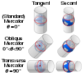
	Normal Mercator		Transverse Mercator
		\

streching

Cylindrical projections in general have an increased vertical stretching as one moves towards either of the poles. Indeed, the poles themselves can't be represented (except at infinity). This stretching is reduced in the  Mercator projection by the natural logarithm scaling. 

truncution

Cylinder is nor finity so Mercator projections give ininite stripes with increasing distorion at poles of sphere. Thus the coordinate y of the Mercator projection becomes infinite at the poles and the map must be truncated ( cropped) at some latitude less than ninety degrees at both ends .

This need not be done symmetrically:

• Mercator's original map is truncated at 80°N and 66°S with the result that European countries were moved toward the centre of the map.

geometry of the earth

earth as sphere

Coordinate systems for the Earth in geography $(\phi ,\lambda )$

• latitude is a coordinate that specifies the north–south position of a point on the surface of the Earth or another celestial body. Latitude is given as an angle that ranges from –90° at the south pole to 90° at the north pole, with 0° at the Equator. is usually denoted by the Greek lower-case letter phi (ϕ or φ). It is measured in degrees, minutes and seconds or decimal degrees, north or south of the equator.
• Longitude is a geographic coordinate that specifies the east–west position of a point on the surface of the Earth. It is an angular measurement, usually expressed in degrees and denoted by the Geek letter lambda (λ).

• 
  A perspective view of the Earth showing how latitude ($\phi$) and longitude ($\lambda$) are defined on a spherical model. The graticule spacing is 10 degrees.

equation

One step method:

Consider a point on the globe of radius R with longitude λ and latitude φ. The value λ₀ is the longitude of an arbitrary central meridian that is usually, but not always, that of Greenwich (i.e., zero). The angles λ and φ are expressed in radians.

Map from point P on the unit sphere $P=(R,\lambda ,\varphi )$ to point on the Cartesian plane $Q=(x,y)$

${\begin{matrix}x=R(\lambda -\lambda _{0})\\y=R\ln \left[\tan \left({\frac {\pi }{4}}+{\frac {\varphi }{2}}\right)\right]\end{matrix}}$

Two step method

• stereographic
• complex log

The spherical form of the stereographic projection is usually expressed in polar coordinates:

${\begin{matrix}r&=2R\tan \left({\frac {\pi }{4}}-{\frac {\varphi }{2}}\right)\\\theta &=\lambda \end{matrix}}$

where $R$ is the radius of the sphere, and $\varphi$ and $\lambda$ are the latitude and longitude, respectively.

rectangular coordinates

Assumption: A, B, C, and D are real numbers such that $A^{2}+B^{2}+C^{2}\neq 0$.

Definitions

• $\Sigma$ is defined to be the unit sphere in the Euclidean space, i.e.

  $\Sigma :={\big \{}(x,y,z)\in \mathbb {R} ^{3}:x^{2}+y^{2}+z^{2}=1{\big \}}.$

• $N$ is defined to be the northern pole of the unit sphere, i.e. $N:=(0,0,1)$.
• $S$ is defined to be the stereographic projection, i.e. the function $S:\Sigma \setminus \{N\}\rightarrow \mathbb {R} ^{2}$ satisfying

  $Q=S{\big (}(x,y,z){\big )}={\Big (}{\frac {x}{1-z}},{\frac {y}{1-z}}{\Big )}$

for every $(x,y,z)\in \Sigma \setminus \{N\}$.

Cylindrical coordinates

Cylindrical coordinates (axial radius ρ, azimuth φ, elevation z) may be converted into spherical coordinates (central radius r, inclination θ, azimuth φ), by the formulas

$${\begin{aligned}r&={\sqrt {\rho ^{2}+z^{2}}},\\\theta &=\arctan {\frac {\rho }{z}}=\arccos {\frac {z}{\sqrt {\rho ^{2}+z^{2}}}},\\\varphi &=\varphi .\end{aligned}}$$

Conversely, the spherical coordinates may be converted into cylindrical coordinates by the formulae

$${\begin{aligned}\rho &=r\sin \theta ,\\\varphi &=\varphi ,\\z&=r\cos \theta .\end{aligned}}$$

These formulae assume that the two systems have the same origin and same reference plane, measure the azimuth angle φ in the same senses from the same axis, and that the spherical angle θ is inclination from the cylindrical z axis.

Code

• chinhsuanwu: 360-converter ( A C/C++ toolkit of 360 image conversions )

Signal processing

Filter Linear continuous-time filters

• The frequency response can be classified into a number of different bandforms describing which frequency bands the filter passes (the passband) and which it rejects (the stopband):
  • Low-pass filter – low frequencies are passed, high frequencies are attenuated.
  • High-pass filter – high frequencies are passed, low frequencies are attenuated.
  • Band-pass filter – only frequencies in a frequency band are passed.
  • Band-stop filter or band-reject filter – only frequencies in a frequency band are attenuated.
  • Notch filter – rejects just one specific frequency - an extreme band-stop filter.
  • Comb filter – has multiple regularly spaced narrow passbands giving the bandform the appearance of a comb.
  • All-pass filter – all frequencies are passed, but the phase of the output is modified.
• Cutoff frequency is the frequency beyond which the filter will not pass signals. It is usually measured at a specific attenuation such as 3 dB.
• Roll-off is the rate at which attenuation increases beyond the cut-off frequency.
• Transition band, the (usually narrow) band of frequencies between a passband and stopband.
• Ripple is the variation of the filter's insertion loss in the passband.
• The order of a filter is the degree of the approximating polynomial and in passive filters corresponds to the number of elements required to build it. Increasing order increases roll-off and brings the filter closer to the ideal response.

time series

smoothing time series data

• Smoothing with a moving average. A moving average filter is sometimes called a boxcar filter, especially when followed by decimation.
  • Exponential smoothing
• Category:Smoothing_(time_series) in commons
• smoothish js program by Eamonn O'Brien-Strain

Ripple voltage from a full-wave rectifier, before and after the application of a smoothing capacitor

Smoothing of a noisy sine (blue curve) with a moving average (red curve).

Faq

• faqs.org: graphics algorithms-faq
• The Arcane Algorithm Archive

References

• c programs from GraphicsGems book
• GraphicsGems - Code for the "Graphics Gems" book series
• Code developed for articles in the "Journal of Graphics Tools"
• https://www.geeksforgeeks.org/fundamentals-of-algorithms/#GeometricAlgorithms
• VTK Book
• Algorithms by Jeff Erickson
• immersive linear algebra by J. Ström, K. Åström, and T. Akenine-Möller