Planet Earth/print version

Table of Contents
Front Matter
Section 1: EARTH’S SIZE, SHAPE, AND MOTION IN SPACE
- a. Science: How do we Know What We Know?
- b. Earth System Science: Gaia or Medea?
- c. Measuring the Size and Shape of Earth
- d. How to Navigate Across Earth using a Compass, Sextant, and Timepiece
- e. Earth's Motion and Spin
- f. The Nature of Time: Solar, Lunar and Stellar Calendars
- g. Coriolis Effect: How Earth’s Spin Affects Motion Across its Surface
- h. Milankovitch cycles: Oscillations in Earth’s Spin and Rotation
- i. Time: The Invention of Seconds using Earth’s Motion
Section 2: EARTH’S ENERGY
- a. Energy and the Laws of Thermodynamics
- b. Solar Energy
- c. Electromagnetic Radiation and Black Body Radiators
- d. Daisy World and the Solar Energy Cycle
- e. Other Sources of Energy: Gravity, Tides, and the Geothermal Gradient
Section 3: EARTH’S MATTER
- a. Gas, Liquid, Solid (and other states of matter)
- b. Atoms: Electrons, Protons and Neutrons
- c. The Chart of the Nuclides
- d. Radiometric dating, using chemistry to tell time
- e. The Periodic Table and Electron Orbitals
- f. Chemical Bonds (Ionic, Covalent, and others means to bring atoms together)
- g. Common Inorganic Chemical Molecules of Earth
- h. Mass spectrometers, X-Ray Diffraction, Chromatography and Other Methods to Determine Which Elements are in Things
Section 4: EARTH’S ATMOSPHERE
- a. The Air You Breathe
- b. Oxygen in the Atmosphere
- c. Carbon Dioxide in the Atmosphere
- d. Green House Gases
- e. Blaise Pascal and his Barometer
- f. Why are Mountain Tops Cold?
- g. What are Clouds?
- h. What Makes Wind?
- i. Global Atmospheric Circulation
- j. Storm Tracking
- k. The Science of Weather Forecasting
- l. Earth’s Climate and How it Has Changed
Section 5: EARTH’S WATER
- a. H2O: A Miraculous Gas, Liquid and Solid on Earth
- b. Properties of Earth’s Water (Density, Salinity, Oxygen, and Carbonic Acid)
- c. Earth’s Oceans (Warehouses of Water)
- d. Surface Ocean Circulation
- e. Deep Ocean Circulation
- f. La Nina and El Nino, the sloshing of the Pacific Ocean
- g. Earth‘s Rivers.
- h. Earth’s Endangered Lakes and the Limits of Freshwater Sources
- i. Earth’s Ice: Glaciers, Ice Sheets, and Sea Ice
Section 6: EARTH’S SOLID INTERIOR
- a. Journey to the Center of the Earth: Earth’s Interior and Core
- b. Plate Tectonics: You are a Crazy Man, Alfred Wegener
- c. Earth’s Volcanoes: When Earth Goes Boom!
- d. You Can’t Fake an Earthquake: How to Read a Seismograph
- e. The Rock Cycle and Rock Types (Igneous, Metamorphic and Sedimentary)
- f. Mineral Identification of Hand Samples
- g. Common Rock Identification
- h. Bowen’s Reaction Series
- i. Earth’s Surface Processes: Sedimentary Rocks and Depositional Environments
- j. Earth’s History Preserved in its Rocks: Stratigraphy and Geologic Time
Section 7: EARTH’S LIFE
- a. How Rare is Life in the Universe?
- b. What is Life?
- c. How did Life Originate?
- d. The Origin of Sex
- e. Darwin and the Struggle for Existence
- f. Heredity: Gregor Mendel’s Game of Cards
- g. Earth’s Biomes and Communities
- h. Soil: Living Dirt
- i. Earth’s Ecology: Food Webs and Populations
Section 8: EARTH’S HUMANS AND FUTURE
- a. Ötzi’s World or What Sustainably Looks Like
- b. Rise of Human Consumerism and Population Growth
- c. Solutions for the Future
- d. How to Think Critically About Earth's Future
Section 1: EARTH’S SIZE, SHAPE, AND MOTION IN SPACE
1a. Science: How do we Know What We Know.
The Emergence of Scientific Thought
The term "science" comes from the Latin word for knowledge, scientia, although the modern definition of science only appears during the last 200 years. Between the years of 1347 to 1351, a deadly plague swept across the Eurasian Continent, resulting in the death of nearly 60% of the population. The years that followed the great Black Death, as the plague came to be called, was a unique period of reconstruction which saw the emergence of the field of science for the first time. Science became the pursuit of learning knowledge and gaining wisdom; it was synonymous with the more widely used term of philosophy. It was born in the time when people realized the importance of practical reason and scholarship in the curing of diseases and ending famines, as well as the importance of rational and experimental thought. The plague resulted in a profound acknowledgement of the importance of knowledge and scholarship to hold a civilization together. An early scientist was indistinguishable from being a scholar.
Two of the most well-known scholars to live during this time was Francesco “Petrarch” Petrarca and his good friend Giovanni Boccaccio; both were enthusiastic writers of Latin and early Italian, and they enjoyed a wide readership of their works of poetry, songs, travel writing, letters, and philosophy. Petrarch rediscovered the ancient writings of Greek and Roman figures of history and worked to popularize them into modern Latin, particularly rediscovering the writings of the Roman statesman Cicero, who had lived more than a thousand years before him. This pursuit of knowledge was something new, both Petrarch and Boccaccio proposed the kernel of thought in a scientific ideal that has transcended into the modern age, that the pursuit of knowledge and learning does not conflict with religious teachings as the capacity of intellectual and creative freedom is in itself divine. Secular pursuit of knowledge based on truth complements faith and religious doctrines which are based on belief and faith. This idea manifested during the Age of Enlightenment and eventually in the American Revolution as an aspiration for a clear separation of church and state. This sense of freedom to pursue knowledge and art, unhindered by religious doctrine, led to the Italian Renaissance of the early 1400s.

The Italian Renaissance was fueled as much by this new freedom to pursue knowledge as it was the global and economic shift that brought wealth and prosperity to northern Italy and later in northern Europe and England. This was a result of the fall of the Byzantine Empire, and the rise of a new merchant class of the city-states of northern Italy which took up the abandoned trade routes throughout the Mediterranean and beyond. The patronage of talented artists and scholars arose during this time as wealthy individuals financed not only artists but also the pursuit of science and technology. The first universities, places of learning outside of monasteries and convents, came into fashion for the first time as wealthy leaders of the city states of northern Italy sought talented artists and inventors to support within their own courts. Artists like Leonard da Vinci, Raphael, and Michelangelo received commissions from wealthy patrons, including the church and city-states, to create realistic artworks from the keen observation of the natural world. Science grew out of art, as the direct observation of the natural world led to deeper insights into the creation of realistic paintings and sculptures. This idea of the importance of observation found in Renaissance art transcended into the importance of observation in modern science today. In other words, science should reflect reality by the ardent observation of the natural world.
The Birth of Science Communication
Science and the pursuit of knowledge during the Renaissance was enhanced to a greater extent by the invention of the printing press with moveable type, allowing the widespread distribution of information in the form of printed books. While block and intaglio prints using ink on hand-carved wood or metal blocks predated this period, re-movable type allowed the written word to be printed and copied onto pages much more quickly. The Gutenberg Bible was first printed in 1455, with 800 copies made in just a few weeks. This cheap and efficient way to replicate the written word had a dramatic effect on society, as literacy among the population grew. It was much more affordable to own books and written works than any previous time in history. With a little wealth, the common individual could pursue knowledge through the acquisition of books and literature. Of importance to science was the newfound ease to which you could disseminate information. The printing press led to the first information age and greatly influenced scientific thought during the middle Renaissance in the second half of the 1400s. Many of these early works were published with the mother tongue, the language spoken in the home, rather than the father tongue, the language of civic discourse found in the courts and the churches of the time, which was mostly Latin. These books spawned the early classic works of literature we have today in Italian, French, Spanish, English, and other European languages spoken across Europe and the world.

One of the key figures of this time was Nicolaus Copernicus, who published his mathematical theory that the Earth orbited around the Sun in 1543. The printed book entitled De revolutionibus orbium coelestium (On the Revolutions of the Celestial Spheres), written in the scholarly father tongue of Latin ushered in what historians called the Scientific Revolution. The book was influential because it was widely read by fellow astronomers across Europe. Each individual could verify the conclusions made by the book by carrying out the observations on their own. The Scientific Revolution was not so much what Nicolaus Copernicus discovered and reported (which will be discussed in depth later) but that the discovery and observations he made could be replicated by others interested in the same question. This single book led to one of the most important principles in modern science, that any idea or proposal must be verified through replication. What makes something scientific is that it can be replicated or verified by any individual interested in the topic of study. Science embodied at its core the reproducibility of observations made by individuals, and this principle ushered in the age of experimentation.
During this period of time, such verifications of observations and experiments was a lengthy affair. Printing costs of books and the distribution of that knowledge was very slow and often subjected to censure. This was also the time of the Reformation, first led by Martin Luther who protested corruption within the Catholic Church, leading to the establishment of the Protestant Movement in the early 1500s. This schism of thought and belief brought about primarily by the printing of new works of religious thought and discourse gave rise to the Inquisition. The Inquisition was a reactionary system of courts established by the Catholic Church to convict individuals who showed signs of dissent from the established beliefs sent forth by doctrine. Printed works that hinted at free thought and inquiry were destroyed and their authors imprisoned or executed. Science, which had flourished in the century before, suffered during the years of the Inquisition, but it also brought about one of the most important episodes in the history of science involving of one of the most celebrated scientists of its day, Galileo Galilei.
The Difference between Legal and Scientific Systems of Inquiry

Galileo was a mathematician, physicist, and astronomer who taught at one of the oldest Universities in Europe—the University of Padua. Galileo got into an argument with a fellow astronomer named Orazio Grassi, who taught at the Collegio Romano in Rome. Grassi had published a book in 1619 on the nature of three comets he had observed from Rome, entitled De tribus cometis anni MDCXVIII (On Three Comets in the Year 1618). The book angered Galileo who argued that comets were an effect of the atmosphere and not real celestial bodies. Although Galileo had invented an early telescope for observing the Moon, planets, and comets, he had not made observations of the three comets observed by Grassi. As a rebuttal, Galileo published his response in a book entitled The Assayer which, in a flourish, he dedicated to the Pope living in Rome. The dedication was meant as an appeal to authority, in which Galileo hoped that the Pope would take his side in the argument.
Galileo was following a legal protocol for science, where evidence is presented to a judge or jury, or Pope in this case, and they decide on a verdict based on the evidence presented before them. This appeal to authority was widely in use during the days of the Inquisition,and still practiced in law today. Galileo in his book The Assayer presented the notion that mathematics is the language of science. Or in other words, the numbers don’t lie. Despite being wrong, the Pope sided with Galileo, which emboldened Galileo to take on a topic he was interested in but was considered highly controversial by the church—the idea that Earth rotated around the Sun proposed by Copernicus. Galileo wanted to prove it using his own mathematics.
Before his position at the university, Galileo had served as a math tutor for the son of Christine de Lorraine the Grand Duchess of Tuscany. Christine was wealthy, highly educated, and more open to the idea of a heliocentric view of the Solar System. In a letter to her, Galileo proposed the rationale for undertaking a forbidden scientific inquiry, invoking the idea that science and religion were separate and that biblical writing was meant to be allegorical. Truth could be found in mathematics, even when it contradicted the religious teachings of the church.
In 1632 Galileo published the book Dialogue Concerning the Two Chief World Systems in Italian and dedicated it to Christine's grandson. The book was covertly written in an attempt to bypass the censors of the time who could ban the work if they found that it was heretical to the teachings of the church. The book was written as a dialogue between three men (Simplicio, Salviati, and Sagredo), who over the course of four days debate and discuss the two world systems. Simplicio argues that the Sun rotates around the Earth, while Salviati argues that the Earth rotates around the Sun. The third man Sagredo, is neutral, and he listens and responds to the two theories as an independent observer. While the book was initially allowed to be published, it raised alarm among members of the clergy, and charges of heresy were brought forth against Galileo after its publication. The book was banned as well as all the previous writings of Galileo. The Pope, who had previously supported Galileo, saw himself as the character Simplicio, the simpleton. Furthermore, a letter to Christine was uncovered and brought forth during the trial. Galileo was found guilty of heresy and excommunicated from the church and placed under house arrest for the rest of his life. Galileo’s earlier appeal to authority appeared to be revoked as he faced these new charges. The result of Galileo’s ordeal was that fellow scientists felt that he had been wrongfully convicted and that the authority, whether religious or governmental, was not the determiner of truth in scientific inquiry.
Galileo’s ordeal established the important principle of the independence of science from authority in the determination of truth in science. The notion of appealing to authority figures should not be a principle of scientific inquiry. Unlike the practice of law, science was governed not by judges or juries, who could be fallible and wrong, nor was it governed through popular public opinion or even voting.
This led to an existential crisis in scientific thought. How can one define truth, especially if you can’t appeal to authority figures in leadership positions to judge what is true?
Scientific Deduction and How to Become a Scientific Expert

The first answer came from a contemporary of Galileo, René Descartes, a French philosopher who spent much of his life in the Dutch Republic. Descartes coined the motto, cogito, ergo sum, I think therefore I am, which was taken from his well-known preface entitled, (Discourse on the Method), published in both French and Latin in 1637. The essay is an exploration of how one can determine truth, and it is a very personal exploration of how he himself determines what is true or not. René Descartes argued for the importance of two principles in seeking truth.
First was the idea that it requires much reading, taking and passing classes, but also exploring the world around you— traveling and learning new cultures and meeting new people. He recommended joining the army, and living not only in books and university classrooms, but also living life in the real world and learning with everything that you do. Truth was based on common sense but only after careful study and work. What Descartes advocated was that expertise in a subject came not only from learning and studying a subject over many years but also practice in the real-world environment. A medical doctor who had never practiced nor read any books on the subject of medicine was a poorer doctor to one who attended many years of classes and kept up to date on the newest discoveries in books and journals and had practiced for many years in a medical office. The expert doctor would be able to discern a medical condition much more readily than a novice. With expertise and learning, one could come closer to knowing the truth.
The second idea was that anyone could obtain this expertise if they worked hard enough. René Descartes basically states that he was a normal average student, but through his experience and enthusiasm for learning more, he was able, over the years, to become expert enough to discern truth from fiction, hence he could claim, I think therefore I am.
What René Descartes advocated was that if you have to appeal to authority, seek experts within the field of study of your inquiry. These two principles of science should be a reminder that in today’s age of mass communication (Twitter, Facebook, Instagram) for everyone, much falsehood is perpetrated by novices in the spread of lies unknowingly, and to combat these lies or falsehoods, one must be educated and well informed through an exploration of written knowledge, educational institutions, and life experiences in the real world, and if you don’t have these, then seek experts.
René Descartes’ philosophy had a profound effect on science, although even he would reference this idea to le bon sens (common sense).
Descartes’ philosophy went further to answer the question of what if the experts are wrong? If two equally experienced experts disagree, how do we know who is right if there is no authority we can call upon to decide? How can one uncover truth through their own inquiry? Descartes’ answer was to use deduction. Deduction is where you form an idea and then test that idea with observation and experimentation. An idea is true until it is proven false.
The Idols of the Mind and Scientific Eliminative Induction
.jpg)
This idea was flipped on its head by a man so brilliant that rumors exist that he wrote William Shakespeare’s plays in his own free time. Although no evidence exists to prove these rumors true, they illustrate how widely regarded he was considered, even today. The man’s name was Francis Bacon, and he advanced the method of scientific inquiry that today we call the Baconian approach.
Francis Bacon studied at Trinity College in Cambridge England, and rose up the ranks to become Queen Elizabeth’s legal advisor, thus becoming the first Queen’s Counsel. This position led Francis Bacon to hear many court cases and take a very active role in interpreting the law on behalf of the Queen’s rule. Hence, he had to devise a way to determine truth on a nearly daily basis. In 1620 he published his most influential work, Novum Organum, (New Instrument). It was a powerful book.
Francis Bacon contrasted his new method of science from those advocated by René Descartes by stating that even experts could be wrong and that most ideas were false rather than true. According to Bacon, falsehood among experts comes from four major sources, or in his words, idols of the mind.
First was the personal desire to be right—the common notion that you consider yourself smarter than anyone else, this he called idola tribus. And it extended to the impression you might have that you are on the right track or had some brilliant insight even if you are incorrect in your conclusion. People cling to their own ideas and value them over others, even if they are false. This could also come from a false idea that your mother, father, or grandparent told you was true, and you held onto this idea more than others because it came from someone you respect.
The second source of falsehood among experts comes from idola specus. Bacon used the metaphor of a cave where you store all that you have learned, but we can use a more modern metaphor, watching YouTube videos or following groups on social media. If you consume only videos or follow writers with a certain worldview you will become an expert on something that could be false. If you read only books claiming that the world is flat, then you will come to a false conclusion that the world is flat. Bacon realized that as you consume information about the world around you, you are susceptible to false belief due to the random nature in what you learn and where you learn those things from.
The third source of falsehood among experts come from what he called idola fori. Bacon said that falsehood resulted from the misunderstanding of language and terms. He said that science, if it seeks truth should clearly define the words that it uses, otherwise even experts will come to false conclusions by their misunderstandings of a topic. Science must be careful to avoid ill-defined jargon, and it should define all terms it uses clearly and explicitly. Words can lie and when used well, can cloak falsehood as truth.
The final source of falsehood among experts results from the spectacle of idola theatri. Even if the idea makes a great story, it may not be true. Falsehood comes within the spectacle of trending ideas or widely held public opinions, which of course come and go based on fashion or popularity. Just because something is widely viewed or, in the modern sense, gone viral on the Internet, does not mean that it is true. Science and truth are not popularity contests nor does it depend on how many people come to see it in theaters, nor how fancy the computer graphics are in the science documentary you watched last night, nor how persuasive the Ted Talk was delivered. Science and truth should be unswayed by public perception and spectacle. Journalism is often engulfed within the spectacle of idola theatri, reporting stories that invoke fear and anxiety to increase viewership and outrage, and often they are untrue.
These four idols of the mind led Bacon to the conclusion that knowing the truth was an impossibility, that in science we can get closer to the truth, but we can never truly know what we know. We all fail at achieving truth. Bacon warned that truth was an artificial construct formed by the limitations of our perceptions and that it is easily cloaked or hidden in falsehood, principally by the Idols of the Mind.
So if we can’t know absolute truth, how can we get closer to the truth? Bacon proposed something philosophers call eliminative induction. Start with observations and experimentations, and using that knowledge to look for patterns, eliminate ideas which are not supported by those observations. This style of science, which starts with observations and experiments, resulted in a profound shift in scientific thinking.
Bacon viewed science as focused on the exploration and the documentation of all natural phenomena. The detailed cataloguing of all things observable, all experiments untaken, and the systematic analysis among multitudes of observations and experiments for threads of knowledge that lead to the truth. While previous scientists proposed theories and then sought out confirmation of those theories, Bacon proposed first making observations and then drawing theories which best fit the observations that had been made.
Francis Bacon realized that this method was powerful, and he proposed the idea that “with great knowledge comes great power.” He had seen how North and South American Empires, such as the Aztecs, had been crushed by the Spanish during the mid-1500s and how knowledge of ships, gun powder, cannons, metallurgy, and warfare had resulted in the fall and collapse of whole civilizations of peoples in the Americas. The Dutch utilized the technology of muskets against North American tribes, focusing on the assassination of its leaders. They also produced the wholesale manufacturing of wampum beads, which destroyed North American currencies and the native economies. Science was power because it provided technology that could be used to destroy nations and conquer people.
He foresaw the importance of exploration and scientific discovery if a nation was to remain of importance in a modern world. With Queen Elizabeth’s death in 1603, Francis Bacon encouraged her successor, King James, to colonize the Americas, envisioning the ideal of a utopian society in a new world. He called this utopian society Bensalem in his unfinished science fiction book New Atlantis. This society would be an industry into pure scientific inquiry, where researchers could experiment and document their observations with finer detail, and from those observations, large-scale patterns and theories could emerge that would lead to new technologies.
Francis Bacon’s utopian ideals took hold within his native England, especially within the Parliament of England under the House of Lords who viewed the authority of the King with less respect than any time in its history. The English Civil War and the execution of its King, Charles I, in 1649 tossed the country of England into chaos, and many people fled to the American Colonies in Virginia during the rise of Thomas Cromwell’s dictatorship.
But with the reestablishment of a monarchy in 1660, the ideas laid out by Francis Bacon came to fruition with the founding of the Royal Society of London for Improving Natural Knowledge, or simply the Royal Society. It was the first truly modern scientific society and it still exists today.
Scientific Societies
A scientific society is dedicated to research and sharing of discovery among its members. They are considered an “invisible college” since scientific societies are where experts in the fields of science come and learn from each other and demonstrate new discoveries and publish new results of experiments that they had conducted. As one of the first scientific societies, the Royal Society in England welcomed not only experiments of grand importance, but also insignificant, small-scale observations at their meetings. The Royal Society received support from its members as well as from the monarchy, Charles II, who viewed the society as a useful source of new technologies where new ideas would have important implementations in both state warfare and commerce. Its members included some of England’s most famous scientists of the time; including Isaac Newton, Robert Hooke, Charles Babbage, and even the American Colonialist Benjamin Franklin. Membership was exclusive to upper class men with English citizenship who could finance their own research and experimentation.
Most scientific societies today are open to membership of all citizens and genders, and they have had a profound influence on the sharing of scientific discoveries and knowledge among its members and the public. In the United States of America, the American Geophysical Union and Geological Society of America rank as the largest scientific societies dedicated to the study of Earth science, but hundreds of other scientific societies exist in the fields of chemistry, physics, biology, and geology. Often these societies hold meetings, where new discoveries are shared with scientists by its members giving presentations, and societies have their own journals which publish research and distribute these journals to libraries and fellow members of the society. These journals are often published as proceedings, which can be read by those who cannot attend meetings in person.
The rise of scientific societies allowed the direct sharing of information and a powerful sense of community among the elite experts in various fields of study. It also put into place an important aspect of science today, the idea of peer review. Before the advent of scientific societies, all sorts of theories and ideas were published in books, and most of these ideas were fictitious to the point that even courts of law favored verbal rather than written testimonies because they felt that the written word was much further from the truth, than the spoken word. Today we face a similar multitude of false ideas and opinions expressed on the Internet. It is easy for anyone to post a web page or express a thought on a subject, you just need a computer and internet connection.
Peer Review
To combat widely spreading fictitious knowledge, the publications of the scientific societies underwent a review system among its members. Before an idea or observation was placed into print in a society’s proceedings, it had to be approved by a committee of fellow members, typically between 3 to 5 members who agreed that it was with merit. This became what we call peer review. A paper or publication that underwent this process was given the stamp of approval among the top experts within that field. Many manuscripts submitted for peer review are never published, as one or more of the expert reviewers may find it lacking evidence and reject it. However, readers found peer-review articles of much better quality than other printed works, and they realized that these works carried more authority than written works that did not go through the process.
Today peer-review articles are an extremely important aspect of scholarly publication, and you can exclusively search among peer-reviewed articles by using many of the popular bibliographical databases or indexes, such as Google’s scholar.google.com, GeoRef published by the American Geosciences Institute, available through library subscription, and Web of Science published by the Canadian based Thomson Reuters Corporation and also available only through library subscription. If you are not a member of a scientific society, retrieved online articles are available for purchase, and many are now accessible to nonmembers for free online depending on the scientific society and publisher of their proceedings. Most major universities and colleges subscribe to these scholarly journals, and access may require a physical visit to a library to read articles.
While peer-reviewed publications carry more weight among experts than news articles and magazines published by the public press, they can be subjected to abuse. Ideas that are revolutionary and progress science and discovery beyond what your current peers believe is true are often rejected from publication because it may prove them wrong. Furthermore, ideas that conform to the current understanding of the peer reviewer’s ideas are often approved for publication. As a consequence, peer review favors more conservatively held ideas. Peer review can be stacked in an author’s favor when their close friends are the reviewers, while a newbie in a scientific society might have much more trouble getting their new ideas published and accepted. The process can be long, with some reviews taking several years to get an article published and accepted. Feuds between members of a scientific society can cause members to fight among themselves over controversial subjects or ideas. Max Planck, a well-known German physicist, lamented that “a new scientific truth does not triumph by convincing its opponents and making them see the light, but rather because its opponents eventually die and a new generation grows up that is familiar with it.” In other words, science progresses one funeral at a time.
Another limitation of peer review is that the articles are often not read outside of the membership of the society. Most local public libraries do not subscribe to these specialized academic journals. Access to these scholarly articles are limited to students at large universities and colleges and members of the scientific society. Scientific societies were seen in the early centuries of their existence as the exclusive realm of privileged, wealthy, high-ranking men, and the knowledge contained in these articles was locked away from the general public. Public opinion of scientific societies, especially in the late 1600s and early 1700s, viewed them as secretive and often associated with alchemy, magic, and sorcery, with limited public engagement of the experiments and observations made by its members.
The level of secrecy rapidly changed during the Age of Enlightenment in the late 1700s and early 1800s with the rise of widely read newspapers which reported to the public on scientific discoveries. The American, French, and Haitian Revolutions likely were brought about as much by a desire for freedom of thought and press as they were fueled by the opening of scientific knowledge and inquiry into the daily lives of the public. Most of the founding members of the United States of America were avocational or professional in their scientific inquiry, directly influenced by the scientific philosophy of Francis Bacon, particularly Thomas Jefferson.
Major Paradigm Shifts in Science
In 1788 the Linnean Society of London was formed, which became the first major society dedicated to the study of biology and life in all its forms. This society get its name from the Swedish biologist Carl Linnaeus, who laid out an ambitious goal to name all species of life in a series of updated books first published 1735. The Linnean Society was for members interested in discovering new forms of life around the world. The great explorations of the world during the Age of Enlightenment resulted in the rising status of the society, as new reports of strange animals and plants were studied and documented.
The great natural history museums were born during this time of discovery to hold physical samples of these forms of life for comparative study. The Muséum National d’histoire Naturelle in Paris was founded in 1793 following the French Revolution. It was the first natural history museum established to store the vast variety of life forms from the planet, and it housed scientists who specialized on the study of life. Similar natural history museums in Britain and America struggled to find financial backing until the mid-1800s, with the establishment of a permanent British Museum of Natural History (now known as the Natural History Museum of London) in the 1830s, as well as the American Museum of Natural History, and Smithsonian Institute following the American Civil War in the 1870s.
The vast search for new forms of life resulted in the discovery by Charles Darwin and Alfred Wallace that through a process of natural selection, life forms can evolve and originate into new species. Charles Darwin published his famous book, On the Origin of Species by Means of Natural Selection in 1859, and like Copernicus before him, science was forever changed. Debate over the acceptance of this new paradigm proposed by Charles Darwin resulted in a schism among scientists of the time, and it developed in a new informal society of his supporters dubbed X Club and lead by Thomas Huxley, who became known as Darwin’s Bulldog. Articles which supported Darwin’s theory were systematically rejected in the established scientific journals of the time, and the members of X Club established the journal Nature, which is today considered one of the most prestigious scientific journals. New major scientific paradigm shifts often result in new scientific societies.
The Industrialization of Science
Public fascination of natural history and the study of Earth grew greatly during this time in the late 1700s and early 1800s, with the first geological mapping of the countryside and naming of layers of rocks. The first suggestions of an ancient age and long history for the Earth were proposed with the discovery of dinosaurs and other extinct creatures by the mid-1800s.
The study of Earth led to the discovery of natural resources such as coal, petroleum, and valuable minerals, and advances in the use of fertilizers and agriculture, which led to the Industrial Revolution.
All of this was due to eliminative induction advocated by Francis Bacon, but it was beginning to reach its limits. Charles Darwin wrote of the importance of his pure love of natural science based solely on observation and the collection of facts coupled with a strong desire to understand or explain whatever is observed. He also had a willingness to give up any hypothesis no matter how beloved it was to him. Darwin distrusted deductive reasoning, where an idea is examined by looking for its confirmation, and he strongly recommended that science remains based on blind observation of the natural world, but he realized that observation without a hypothesis, without a question, was foolish. For example, it would be foolish to measure the orientation of every blade of grass in a meadow, just for the sake of observation. The act of making observations assumed that there was a mystery to be solved, but the solution of which should remain unverified until all possible observations are made.
Darwin was also opposed to the practice of vivisection, the cruel practice of making observations upon experiments and dissections on live animal's or people that would lead to an animal or person’s suffering pain or death. There was a dark side to Francis Bacon’s unbridled observation when it came to experimenting on living people and animals without ethical oversight. Mary Shelley’s novel Frankenstein published in 1818 was the first of a common literary trope of the mad scientist and the unethical pursuit of knowledge through the practice of vivisection and the general cruelty of experimentation on people and animals. Yet these experiments advanced knowledge, particularly in medicine, and they still remain an ethical issue science grapples with even today.
Following the American Civil War and into World War I, governments became more involved in the pursuit of science than they had in any prior time, with the founding of federal agencies for the study of science, including maintaining the safety of industrially produced food and medicine. The industrialization of the world left citizens dependent on the government for oversight in the safety of food that was purchased for the home rather than grown at the home. New medicines which were addictive or poisonous were tested by governmental scientists before they could be sold. Governments mapped in greater detail their borders with government-funded surveys, and charted trade waters for the safe passage of ships. Science was integrated into warfare and the development of airplanes, tanks, and guns. Science was assimilated within the government, which funded its pursuits, as science became instrumental to the political ambitions of nations.
However, freedom of inquiry and the pursuit of science through observation was restricted around the rise of authoritarianism and national identity. Fascism arose in the 1930s through the dissemination of falsehoods which stoked hatred and fear upon the populations of Europe and elsewhere. The rise of propaganda using the new media of radio and later television nearly destroyed the world of the 1940s, and the scientific pursuit of pure observation was not enough to question political propaganda.
The Modern Scientific Method

During the 1930s, Karl Popper, who watched the rise of Nazi fascism in his native Austria, set about codifying a new philosophy of science. He was particularly impressed by a famous experiment conducted on Albert Einstein’s theory of general relativity. In 1915 Albert Einstein proposed, using predications on the orbits of planets in the Solar System, that large masses aren’t just attracted to each other but that matter and energy are curving the very fabric of space. To test the idea of curved space, scientists planned to study the position of the stars in the sky during a solar eclipse. If Einstein’s theory was correct, the star’s light would bend around the Sun, resulting in an apparent new position of the stars around the Sun, and if he was incorrect, the stars would remain in the same position. In 1919 Arthur Eddington led a trip to Brazil to observe a total solar eclipse and using a telescope he confirmed that the stars’ positions did change during the solar eclipse due to general relativity. Einstein was right! The experiment was in all the newspapers, and Albert Einstein went from an obscure physicist to a someone synonymous with genius.
Influenced by this famous experiment, Karl Popper dedicated the rest of his life to the study of scientific methods as a philosopher. Popper codified what made Einstein’s theory and Eddington’s experiment “scientific.” It carried the risk of proving his idea wrong. Popper wrote that in general what makes something scientific is the ability to falsify an idea through experimentation. Science is not just the collection of observations, because if you view it under the lens of a proposed idea you are likely to see confirmation and verification everywhere. Popper wrote “the criterion of the scientific status of a theory is it's falsifiability, or refutability, or testability” in his 1963 book Conjectures and Refutations. And as Darwin wrote, a scientist must give up their theory if it is falsified through observations, and if a scientist tries to save it with ad hoc exceptions, it destroys the scientific merit of the theory.
Popper developed the modern scientific method that you find in most school textbooks: a formulaic recipe where you come up with a testable hypothesis, you carry out an experiment which either confirms the hypothesis or refutes it, and then you report your results. Scientific writing shifted during this time to a very structured format —introduce your hypothesis, describe your experimental methods, report your results, and discuss your conclusions. Popper also developed a hierarchy of scientific ideas; with the lowest being hypotheses, which are unverified testable ideas, above which sat theories, which are verified through many experiments, and finally principles, which have been verified to such an extent that no exception has ever been observed. This does not mean that principles are truth, but they are supported by all observations and attempts at falsification.
Popper drew a line in the sand to distinguish what he called science and pseudoscience. Science is falsifiable whereas pseudoscience is unfalsifiable. Once a hypothesis is proven false, it should be rejected, but this does not mean that it should be abandoned.
For example, a hypothesis might be “Bigfoot exists in the mountains of Utah.” The test might be “Has anyone ever captured a bigfoot?” with the result “No”, then “Bigfoot does not exist.” However, this does not mean that we stop looking for Bigfoot, but that it is not likely this hypothesis will be supported. However, if someone continues to defend the idea that Bigfoot exists in the mountains of Utah, despite the lack of evidence, the idea moves into the realm of pseudoscience, where as "Bigfoot does not exist" moves into the realm of science. There is a greater risk that someone will find a Bigfoot and prove it wrong, but if you cling to the idea that Bigfoot exists without evidence, then it is not science, it is pseudoscience, because it is now unfalsifiable.
How Governments Can Awaken Scientific Discovery

On August 6 and 9 1945, the United States dropped atomic bombs on the cities of Hiroshima and Nagasaki in Japan, ending World War II. It sent a strong message that scientific progress was powerful. Two weeks before the dramatic end of the war, Vannevar Bush wrote to President Franklin Roosevelt that “scientific progress is one essential key to our security as a nation, to our better health, to more jobs, to a higher standard of living, and to our cultural progress.”
What Bush proposed was that funds should be set aside for pure scientific pursuit which would cultivate scientific research within the United States of America, and he drafted his famous report called Science, the Endless Frontier. From the recommendations in the report, five years later in 1950, the United States government created the National Science Foundation for the promotion of science. Unlike agency or military scientists, which were full-time employees, the National Science Foundation offered grants to scientists for the pursuit of scientific questions. It allowed funding for citizens to pursue scientific experiments, travel to collect observations, and carry out scientific investigations of their own.
The hope was that these grants would cultivate scientists, especially in academia, and that they could be called upon during times of crisis. Funding was determined by the scientific process of peer review rather than the legal process of appeal to authority. However, the National Science Foundation has struggled since its inception as it has been railed against by politicians with a legal persuasion, who argue that only Congress or the President should be the ones to decide what scientific questions are deserving funding. Most government science funding supports military applications as funded directly by politicians, rather than panels of independent scientists, as demonstrated by finances of most governments.
How to Think Critically in a Media Saturated World
During the post war years until the present time, false ideas were not only perpetrated by those in authority but also by the meteoritic rise of advertising—propaganda designed to sell things.
With mass media of the late 1900s and even today, the methods of science inquiry become more important in combating falsehood, not only among those who practiced science, but also the general public. Following modern scientific methods skepticism became a vital tool in not only science, but critical thinking and the general pursuit of knowledge. Skepticism assumes that everyone is lying to you, but people are especially prone to lie to you when selling you something. The common midcentury phrase “there's a sucker born every minute” exalted the pursuit of tricking people for profit, and to protect yourself from scams and falsehood, one needs to become skeptical.
To codify this in a modern scientific framework, Carl Sagan developed his “baloney detection kit”, outlined in his book The Demon-Haunted World: Science as a Candle in the Dark. A popular Professor at Cornell University in New York, Sagan, best known for his television show Cosmos had been diagnosed with cancer when he set out to write his final book. Sagan worried that like a lit candle in the dark, science could be extinguished if not put into practice.
He was aghast to learn that the general public believed in witchcraft, magic stones, ghosts, astrology, crystal healing, holistic medicine, UFOs, Bigfoot and the Yeti, sacred geometry, and opposition to vaccination and the inoculation of cured diseases. He feared that with a breath of wind, scientific thought would be extinguished by the widespread belief in superstition. To prevent that, before his death in 1996 he left us with this “baloney detection kit”, a method of skeptical thinking to help evaluate ideas:
- Wherever possible, there must be independent confirmation of the “facts.”
- Encourage substantive debate on the evidence by knowledgeable proponents of all points of view.
- Arguments from authority carry little weight—“authorities” have made mistakes in the past. They will do so again in the future. Perhaps a better way to say it is that in science, there are no authorities; at most, there are experts.
- Spin more than one hypothesis. If there’s something to be explained, think of all the different ways in which it could be explained. Then think of tests by which you might systematically disprove each of the alternatives.
- Try not to get overly attached to a hypothesis just because it’s yours. It’s only a way station in the pursuit of knowledge. Ask yourself why you like the idea. Compare it fairly with the alternatives. See if you can find reasons for rejecting it. If you don’t, others will.
- Quantify. If whatever it is you are explaining has some measure, some numerical quantity attached to it, you’ll be much better able to discriminate among competing hypotheses. What is vague and qualitative is open to many explanations. Of course, there are truths to be sought in the many qualitative issues we are obliged to confront, but finding them is more challenging.
- If there’s a chain of argument, every link in the chain must work (including the premise) — not just most of them.
- Occam’s razor. This convenient rule-of-thumb urges us when faced with two hypotheses that explain the data equally well to choose the simpler.
- Always ask whether the hypothesis can be, at least in principle, falsified. Propositions that are untestable, unfalsifiable, are not worth much. You must be able to check assertions out. Inveterate skeptics must be given the chance to follow your reasoning, to duplicate your experiments, and see if they get the same result.
The baloney detection kit is a causal way to evaluate ideas through a skeptical lens. This kit borrows heavily from the scientific method but has enjoyed a wider adaption outside of science as a method in critical thinking.
Carl Sagan never witnessed the incredible growth of mass communication through the development of the Internet at the turn of the last century and the rapidity of how information could be shared globally instantaneously which has become a powerful tool, both in the rise of science but also propaganda.
Accessing Scientific Information
The newest scientific revolution of the early 2000s regards the access to scientific information and the breaking of barriers to free inquiry. In the years leading up to the Internet, scientific societies relied on traditional publishers to print journal articles. Members of the societies would author new works as well as review other submissions for free and on a voluntary basis. The society or publisher would own the copyright to the scientific article which was sold to libraries and institutions for a profit. Members would receive a copy as part of their membership fees. However, low readership for these specialized publications with high printing costs resulted in expensive library subscriptions for these publications.
With the advent of the Internet in the 1990s, traditional publishers begin scanning and archiving their vast libraries of copyright content onto the Internet, allowing access through paywalls. University libraries with an institutional subscription account would allow students to connect through a university library to access articles while locking the content of the archival articles beyond paywalls to the general public.
Academic scientists were locked into the system because tenure and advancement within universities and colleges was dependent on their publication record. Traditional publications carried higher prestige, despite having low readership.
Publishers exerted a huge amount of control on who had access to scientific peer-reviewed articles, and students and aspiring scientists at universities were often locked out of access to these sources of information. There was a need to revise the peer-review traditional model.
Open Access and Science
One of the most important originators of a new model for the distribution of scientific knowledge was Aaron Swartz. In 2008 Swartz published a famous essay entitled Guerilla Open Access Manifesto, and led a life as an activist fighting for free access to scientific information online. Swartz was fascinated with online collaborative publications, such as Wikipedia. Wikipedia was assembled by gathering information from volunteers who contribute articles on topics. This information is verified and modified by large groups of users on the platform who keep the website up to date. Wikipedia grew out of a large user community, much like scientific societies, but with an easy entry to contribute new information and edit pages. Wikipedia quickly became one of the most visited sites on the internet in the retrieval of factual information. Swartz advocated for open access, and that all scientific knowledge should be accessible to anyone. He petitioned for Creative Commons Licensing and strongly encouraged scientists to publish their knowledge online without copyrights or restrictions to share that information.
Open access had its adversaries in the form of law enforcement, politicians and governments with nationalist or protectionist tendencies, and private companies with large revenue streams from intellectual property. These adversaries to Open access argued that scientific information could be used to make illicit drugs, new types of weapons, hack computer networks, encrypt communications and share state secrets and private intellectual properties. But it was private companies with large sources of intellectual property who worried the most about the open access movement, lobbying politicians to enact stronger laws to prohibit the sharing of copyright information online.
In 2010 Aaron Swartz used a computer located at MIT’s Open Campus to download scientific articles from the publisher JSTOR, using an MIT computer account. After JSTOR noticed a large surge of online request from MIT it contacted campus police. The campus police arrested Swartz, and he was charged with 35 years in prison and $1,000,000 in fines. Faced with the criminal charges, Swartz committed suicide in 2013.
The repercussions of Aaron Swartz’s ordeal pushed scientists to find alternative ways to distribute scientific information to the public, rather than relying on corporate for-profit publishers. The open access movement was ignited and radicalized, but details even today are still being worked out among various groups of scientists.
The Ten Principle Sources of Scientific Information
There are ten principle sources of scientific information you will encounter, each one should be viewed with skepticism. These sources of information can be ranked based on a scale of the reliability of the information they present. Knowing the original source can be difficult to determine, but by organizing the sources into these ten categories, you can distinguish the relative level of truthfulness of information presented. All of them report some level of falsehood, however, the higher the ranking the more likely the material contains less falsehoods and approaches more truthful statements.
- 1. Advertisements and Sponsored Content
- Any content that is intended to sell you something and made with the intention of making money. Examples include commercials on radio, television, printed pamphlets, paid posts on Facebook and Twitter, sponsored YouTube videos, web page advertisements, and spam email and phone calls. These sources are the least reliable sources of truthfulness.
- 2. Personal Blogs or Websites
- Any content written by a single person without any editorial control or any verification by another person. These include personal websites, YouTube videos, blog posts, Facebook, Twitter, Reddit posts and other online forums, and opinion pieces written by single individuals. These sources are not very good sources of truthfulness, but they can be insightful in specific instances.
- 3. News Sources
- Any content produced by a journalist with the intention of maintaining interest and viewership with an audience. Journalism is the production and distribution of reports on recent events, and while subjected to a higher standard of fact checking (by an editor or producer), they are limited by the need to maintain interest with an audience who will tune in or read its content. News stories tend to be shocking, scandalous, feature famous individuals, and address trending or controversial ideas. They are written by nonexperts who rely on the opinion of experts who they interview. Many news sources are politically orientated in what they report. Examples of new sources are cable news channels, local and national newspapers, online news websites, aggregated news feeds, and news reported on the radio or broadcast television. These tend to be truthful but often with strong biases on subjects covered, factual mistakes and errors, and a fair amount of sensationalism.
- 4. Trade Magazines or Media
- Any content produced on a specialized topic by freelance writers who are familiar with the topic which they are writing about. Examples include magazines which cover a specialized topic, podcasts hosted by experts in the field, and edited volumes with chapters contributed by experts. These tend to have a higher level of truthfulness because the writing staff who create the content are more familiar with the specialized topics covered, with some editorial control over the content.
- 5. Books
- Books are lengthy written treatments on a topic, which require the writer to become familiar with a specific subject of interest. Books are incredible sources of information and are insightful to readers wishing to learn more about a topic. They also convey information that can be inspirational. Books are the result of a long-term dedication on behalf of an author or team of authors, who are experts on the topic or become experts through the research that goes into writing a book. Books encourage further learning of a subject and have a greater depth of content than other sources of information. Books require editorial oversight if its contents are published traditionally. One should be aware that authors can write with a specific agenda or point of view, which may express falsehoods.
- 6. Collaborative Publications or Encyclopedias
- These are sources of scientific information produced by teams of experts with the specific intention of presenting a consensus on a topic. Since the material presented must be subjected to debate, they tend to carry more authority as they must satisfy skepticism from multiple contributors on the topic. Examples of these include Wikipedia, governmental agency reports, reports by the National Academy of Sciences, and the United Nations.
- 7. Preprints, Press Releases, and Meeting Abstracts
-
- Preprints
- Preprints are manuscripts submitted for peer review, but made available online to solicit additional comments and suggestions by fellow scientists. In the study of the Earth, the most common preprint service is eartharxiv.org. Preprints are often picked up by journalists and reported as news stories. Preprints are a way for scientists to get information conveyed to the public more quickly than going through full peer review, and they help establish a precedent by the authors on a scientific discovery. They are a fairly recent phenomenon in science, first developed in 1991 with arxiv.org (pronounced archive) a moderated web service which hosts papers in the fields of science.
- Press Releases
- Press releases are written by staff writers at universities, colleges, and government agencies when an important research study is going to be published in a peer-review paper. Journalist will often write a story based on the press release, as they are written for a general audience and avoid scientific words and technical details. Most press releases will link to the scientific peer-reviewed paper that has been published, so you should also read the referenced paper.
- Meeting Abstracts
- Meeting abstracts are short summaries of research that are presented at scientific conferences or meetings. These are often reported on by journalists who attend the meetings. Some meeting abstracts are invited, or peer reviewed, before scientists are allowed to present their research at the meeting, others are not. Abstracts represent ongoing research that is being presented for scientific evaluation. Not all preprints, and meeting abstracts will make it through the peer-review process, and while many ideas are presented in these formats, not all will be published with a followup paper. In scientific meetings, scientists can present their research as a talk or as a poster. Recordings of the talks are sometimes posted on the Internet, while copies of the posters are sometimes uploaded as preprints. Meeting abstracts are often the work of graduate or advanced undergraduate students who are pursuing student research on a topic.
- 8. Sponsored Scholarly Peer-Review Articles with Open Access
- Sponsored scholarly peer review articles with open access are publications that are selected by an editor and peer-reviewed, but the authors pay to publish the article with the journal, if accepted. Technically these are advertisements or sponsored content since there is an exchange of money from the author or creator of the material to the journal, who allows the article to be accessible to the public on the journal’s website, however, their intention is not to sell a product. With the open access movement, many journals publish scholarly articles in this fashion since the published articles are available to the public to read, free of charge. However, there is abuse. The Beall’s List was established to list predatory or fraudulent scholarly journals that actively solicit scientists and scholars but don’t offer quality peer review and hosting in return of money exchanged for publication. Not all sponsored scholarly peer review articles with open access are problematic, and many are well respected, as many traditional publications offer options to allow public access to an article in exchange of money from the authors. The publication rates for these journals vary greatly between publishers, asking for a few hundred dollars up to the price of a new car. Large governments and well-funded laboratories tend to publish in the more expensive open access journals, which often offer press releases and help publicize their work on social media.
- 9. Traditional Scholarly Peer-Review Articles behind a Paywall
- Most scholarly scientific peer-reviewed articles are written in traditional journals. These journals earn income only from subscriptions from readers, rather than authors paying to publish their works. Authors and reviewers are not paid any money, and there is no exchange of money to publish in these journals. They are reviewed by 3 to 5 expert reviewers who are contacted by the editor to review the manuscript before any consideration of publication. Copyright is held by the journal, and individual articles can be purchased online. Many university and college libraries will have institutional online and print subscriptions with specific journals, so you can borrow a physical copy of the journal from the library if you like to read the publication. Older back issues are often available for free online when the copyright has expired. Most scientific articles are published in this format.
- 10. Traditional Scholarly Peer-Review Articles with Open Access
- These journals are operated by volunteers, allowing authors to submit works for consideration to peer-review, and are not required to pay any money to the journal if the article is accepted for publication. Editors and reviewers work on a voluntary basis, with web hosting services provided by endowments and donations. Articles are available online for free downloading by the general public without any subscription to the journal and are open access. Copyright can be retained by the author or journal or distributed under a Creative Commons License. These journals are rarer, because they are operated by a volunteer staff of scientists.
Researchers studying a topic will often limit themselves to sources 5 through 10 as acceptable sources of information while others may be more restrictive and consult only 8 through 10 sources or only fully peer-reviewed sources. Any source of information can present falsehoods and any source can touch upon truth, but the higher the scale in this scheme, the more verification the source had to go through to get published.
Imagine that a loved one is diagnosed with cancer, and you want to learn more about the topic. Most people will consult sources 1 through 3, or 1 through 5, but if you want to learn what medical professionals are reading, sources above 5 are good sources to read since they are more likely verified by experts than lower ranking sources of information. The higher the ranking, the more technical the writing will be and the more specific the information will be. Remember it is important that you consult many sources of information to verify that the information you consume is correct.
Why We Pursue Scientific Discovery
Hope Jahren wrote in her 2016 book Lab Girl, “science has taught me that everything is more complicated than we first assume, and that being able to derive happiness from discovery is a recipe for a beautiful life.” In a modern world where it appears that everything has been discovered and explored, and everything ever known has been written down by someone, it is refreshing to know that there are still scientific mysteries to discover.
For a budding scientist it can be incredibly daunting as you learn about science. The more you learn about a scientific topic, the more you become overwhelmed by its complexity. Furthermore, any new scientific contribution you make is often met with extreme criticism from scientific experts. Scientists are taught to be overly critical and skeptical of new ideas, and they rarely embrace new contributions easily, especially from someone new to the field. Too frequently young scientists are told by experts what to study and how to study it, but science is still a field of experimentation, observation, and exploration. Remember, science should be fun. The smallest scientific discovery often leads to the largest discoveries.
Hope Jahren discovered that hackberry trees have seeds which are made of calcium carbonate (aragonite), while this is an interesting fact alone, it opened the door onto a better understanding of past climate change, since oxygen elements in aragonite crystals can be used to determine the annual growing temperature of the trees that produced them. This discovery allowed scientists to determine the climate whenever hackberry trees dropped their seeds, even in rock layers millions of years old, establishing a long record of growing temperatures extending millions of years into the Earth’s past.
Such discoveries lead to the metaphor that scientists craft tiny keys that unlock giant rooms, and it is not until the door is unlocked that people, even fellow scientists, realize the implications of the years of research used to craft the tiny key. So, it is important to derive happiness from each and every scientific discovery you make, no matter how small or how insignificant it may appear. Science and actively seeking new knowledge and new experiences will be the most rewarding pursuit of your life.
| Previous | Current | Next | |
|---|---|---|---|
1b. Earth System Science: Gaia or Medea?
Earth as a Puddle
“Imagine a puddle waking up one morning and thinking, ‘This is an interesting world I find myself in — an interesting hole I find myself in — fits me rather neatly, doesn’t it? In fact it fits me staggeringly well, must have been made to have me in it!’ This is such a powerful idea that as the sun rises in the sky and the air heats up and as, gradually, the puddle gets smaller and smaller, frantically hanging on to the notion that everything’s going to be alright, because this world was meant to have him in it, was built to have him in it; so the moment he disappears catches him rather by surprise. I think this may be something we need to be on the watch out for.”

In December 1968, Astronaut William A. Anders on Apollo 8 took a picture of the Earth rising above the Moon’s horizon. It captured how small Earth is when viewed from space, and this image suddenly had a strange effect on humanity. Our planet, our home, is a rather small, insignificant place when viewed from the great distance of outer space. Our lives are collectively from the perspective of Earth looking outward, but with this picture, taken above the surface of the Moon looking back at us, we realized that our planet is really just a small place in the universe.
Earth system science was born during this time in history, in the 1960s, when the exploration of the moon and other planets, allowed us to turn the cameras back on Earth and study it from afar. Earth system science is the scientific study of Earth’s component parts and how these components —the solid rocks, liquid oceans, growing life-forms, and gaseous atmosphere—function, interact, and evolve, and how these interactions change over long timescales. The goal of Earth system science is to develop the ability to predict how and when those changes will occur from naturally occurring events, as well as in response to human activity. Using the metaphor of Douglas Adams’ salient puddle above, we don’t want to get surprised if our little puddle starts to dry up!
A system is a set of things working together as parts of a mechanism or an interconnecting network, and Earth system science is interested in how these mechanisms work in unison with each other. Scientists interested in these global questions simplify their study into global box models. Global box models are analogies that can be used to help visualize how matter and energy move and change across an entire planet from one place or state to another.

For example, the global hydrological cycle can be illustrated by a simple box model, where there are three boxes, representing the ocean, the atmosphere, and lakes and rivers. Water evaporates from the ocean into the atmosphere where it forms clouds. Clouds in the atmosphere rain or snow on the surface of the ocean and land filling rivers and lakes (and other sources of fresh water), which eventually drain into the ocean. Arrows between each of the boxes indicate the direction that water moves between these categories. Flux is the rate at which matter moves from one box into another, which can change depending on the amount of energy. Flux is a rate, which means that it is calculated as a unit over time, in the case of water, this could be determined as volume of water that it rains or snows per year.
There are three types of systems that can be modeled. Isolated systems, in which energy and matter cannot enter into the model from the outside. Closed systems, in which energy, but not matter, can enter into the model, and open systems, in which both energy and matter can enter into the model from elsewhere.
Global Earth systems are regarded as closed systems since the amount of matter entering Earth from outer space is a tiny fraction of the total matter that makes up the Earth. In contrast, the amount of energy from outer space, in the form of sunlight, is large. Earth is largely open to energy entering the system and closed to matter. (Of course, there are rare exceptions to this when meteorites from outer space strike the Earth.)
In our global hydrological cycle, if our box model was isolated, allowing no energy and no matter to enter the system, there would be no incoming energy for the process of evaporation, and the flux rate between the ocean and atmosphere would decrease to zero. In isolated systems with no exchange of energy and matter, over time they will slow down and eventually stop functioning, even if they have an internal energy source. We will explore why this happens when we discuss energy. If the box model is open, such as if ice-covered comets frequently hit the Earth from outer space, there would be a net increase in the total amount of water in the model, or if water was able to escape into outer space from the atmosphere, there would be a net decrease in the total amount of water in the model over time. So it is important to determine if the model is truly closed or open to both matter and energy.
In box models we also want to explore all possible places where water can be stored, for example, water on land might go underground to form groundwater and enter into spaces beneath Earth’s surface, hence we might add an additional box to represent groundwater and its interaction with surface water. We might want to distinguish water locked up in ice and snow by adding another box to represent frozen water resources. You can begin to see how a simple model can, over time, become more complex as we consider all the types of interactions and sources that may exist on the planet.
A reservoir is a term used to describe a box which represents a very large abundance of matter or energy relative to other boxes. For example, the world’s ocean is a reservoir of water because most of the water is found in the world’s oceans. A reservoir is relative and can change if the amount of energy or matter in the source decreases in relation to other sources. For example, if solar energy from the sun increased and the oceans boiled and dried away, the atmosphere would become the major reservoir of water for the planet since the portion of water locked in the atmosphere would be more than found in the ocean. In a box model, a reservoir is called a sink when more matter is entering the reservoir than is leaving it, while a reservoir is called a source if more matter leaves the box than is entering it. Reservoirs are increasing in size when they are a sink and decreasing in size when they are a source.
Sequestration is a term used when a source becomes isolated and the flux between boxes is a very slow rate of exchange. Groundwater, which represents a source of water isolated from the ocean and atmosphere, can be considered an example of sequestration. Matter and energy which is sequestrated have very long residence times, the length of time energy and matter reside in these boxes.
Residence times can be very short, such as a few hours when water from the ocean evaporates, then falls back down into the ocean as rain; or very long, such as a few thousand years when water is locked up in ice sheets and even millions of years underground. Matter that is sequestered is locked up for millions of years, such that it is taken out of the system.
An example of sequestration is an earth system box model of salt (NaCl), or sodium chloride. Rocks weather in the rain, resulting in the dissolution of sodium and chloride, which are transported to the ocean dissolved in water. The ocean is a reservoir of salt since salt will accumulate over time by the process of the continued weathering of the land. Edmund Halley (who predicted a comet’s return and was later posthumously named after him) proposed in 1715 that the amount of salt in the oceans is related to the age of the Earth, and he suggested that salt has been increasing in the world’s ocean over time, which will become saltier and saltier into the future. However, this idea was proved false when scientists determined that the world’s oceans have maintained a similar salt content over its history. There had to be a mechanism to remove salt from ocean water. The ocean loses salt through the evaporation of shallow seas and landlocked water. The salt left behind from the evaporation of the water in these regions is buried under sediments and becomes sequestered underground. The flux of incoming salt into the ocean from weathering is similar to the flux leaving the ocean by the process of evaporated salt being buried. This buried salt will remain underground for millions of years. The salt cycle is at an equilibrium, as the oceans maintain a fairly persistent rate of salinity. The sequestration of evaporated salt is an important mechanism that removes salt from the ocean. Scientists begin to wonder if Earth exhibits similar mechanisms that maintain an equilibrium through a process of feedbacks.
Equilibrium is a state in which opposing feedbacks are balanced and conditions remain stable. To illustrate this, imagine a classroom which is climate controlled with a thermostat. When the temperature in the room is above 75 degrees Fahrenheit, the air conditioner turns on, when the temperature in the room is below 65 degrees Fahrenheit, the heater turns on. The temperature within the classroom will most of the time be at equilibrium between 65 and 75 degrees Fahrenheit, as the heater and air conditioner are opposing forces that keep the room in a comfortable temperature range. Imagine now that the room becomes filled with students, which increase the temperature in the room when the room reaches 75 degrees Fahrenheit, the air conditioner turns on, cooling the room. The air conditioner is a negative feedback. A negative feedback is where there is an opposing force that reduces fluctuations in a system. In this example, the increase in the heat of the students in the room is opposed by the cooling of the air conditioner system turning on.
Imagine that a classmate plays a practical joke, and switches the thermostat. When the temperature in the room is above 75 degrees Fahrenheit, the heater turns on, when the temperature in the room is below 65 degrees Fahrenheit, the air conditioner will turn on. With this arrangement, when students enter the classroom and the temperature slowly reaches 75 degrees Fahrenheit, the heater turns on! The heater is a positive force in the same direction as the heat produced by the students entering the room. A positive feedback is where there are two forces that join together in the same direction, which leads to instability of a system over time. The classroom will get hotter and hotter, even if the students leave the room, the classroom will remain hot, since there is no opposing force to turn on the air conditioner. It likely will never drop down to 65 degrees Fahrenheit, with the heater turned on. Positive feedbacks are sometimes referred to as vicious cycles. The tipping point in our example is 75 degrees Fahrenheit, when the positive feedback (the heater) turned on, resulting in the instability of the system and leading to a very miserable hot classroom experience. Tipping points are to be avoided if there are systems in place with positive feedbacks.
Gaia or Medea?
One of the most important discussions within Earth system science is whether the Earth exhibits mostly negative feedbacks or positive feedbacks and how well regulated are these conditions that we find on Earth today. The two hypotheses are named after two figures in Greek mythology, Gaia the Goddess of Earth, and Medea lover of Jason, who murdered her own children. The Gaia hypothesis maintains that the global Earth system maintains an equilibrium or long-term stability through various negative feedbacks that oppose destabilization of the planet. The Medea hypothesis maintains that the global Earth system does not maintain a stable equilibrium resulting in frequent episodes of catastrophic events. From a geological point of view, the Gaia hypothesis predicts Uniformitarianism, that past geological processes through time have mostly remained continuous and uniform, while the Medea hypothesis predicts Catastrophism, where most past geological processes are the result of sudden, short-lived, and violent events.


This dichotomy of the optimistic view of the Gaia hypothesis and pessimistic Medea hypothesis is a simplification. In reality the true Earth system likely exhibits both types of negative feedbacks and positive feedbacks that interact in complex ways.
Imagine a classroom, now equipped with two thermostats, a normal negative feedback that turns on the air conditioner when the room gets above 75 degrees, and a malfunctioning positive feedback that turns on the heater when the room gets above 80 degrees. Assuming that the classroom begins with a temperature of 70 degrees, and each student who enters the classroom raises the temperature by 1 degree. The air conditioning will turn on when 5 students enter the classroom. This air conditioner is weak and only lowers the temperature by 1 degree every 10 minutes.
The classroom will maintain an equilibrium temperature as long as the rate of students entering the room is below 10 students per 100 minutes. For example, if 7 students entered the classroom at the same time, the temperature would rise by 7 degrees, to 77 degrees—turning on the air conditioner when it crossed 75 degrees and taking 20 minutes to lower the temperature back down to 75 degrees. Another 4 students could enter the classroom, raising the temperature to 79 degrees, turning on the air conditioner and lowering the temperature down to 75 degrees in 40 minutes.
However, if 12 students enter the room at the same time, the temperature will rise to 82 degrees, turning on both the air conditioner at 75 degrees and heater at 80 degrees, the heater warms the room faster (+2 degrees every 10 minutes) than the air conditioner is able to cool the room (−1 degree every 10 minutes). This positive feedback will cause the classroom to increase in temperature until it is a hot oven because the net temperature will increase +1 degree every 10 minutes. The tipping point was when the 12 students entered the room all at once, which set off this vicious cycle of a positive feedback. If the rate of students entering the classroom remains low, the room temperature will remain stable, and it appears to be governed by the Gaia hypothesis. However, if the rate of students entering the classroom is fast, the temperature could become unstable, as governed by the Medea hypothesis.
In determining the mechanisms of how Earth systems play out over time, we also need to be aware of the fallacy of the salient puddle at the beginning of this chapter—a puddle that believes it is perfectly tailored to the environment it finds itself in. The Gaia hypothesis views the Earth as a perfectly working system that is able to adjust to changes and maintain an equilibrium state. This is similar to the salient puddle believing that it fits perfectly within the environment that it finds itself within. In contrast, the Medea hypothesis views that there will inevitably be an event that dries up the puddle, and that the puddle is not at equilibrium under a warm sun.
Who Came Up with These Ideas?
The Gaia hypothesis, has a longer pedigree, and was first formulated in the 1970s by James Lovelock and Lynn Margulis. Initially called the Earth feedback hypothesis, the name Gaia was proposed by the writer William Golding, the author of Lord of the Flies and close neighborhood friend of Lovelock. Lovelock was an expert on air quality and respiratory diseases in England, but he took up the study of the Earth’s sulfur cycle, noting negative feedbacks that appeared to regulate cloud cover. In the 1970s, he had been invited to work on the Viking Missions to Mars by NASA to evaluate the Martian atmosphere for the possible presence of life. Lovelock suggested that if the Viking lander found significant oxygen in the Martian atmosphere it would be indicative of life existing there. Instead the Viking lander found that the Martian atmosphere was 96% carbon dioxide, similar to the atmosphere of Venus. Working with Lynn Margulis, the two formulated a hypothesis that there were natural negative feedback systems on Earth that kept both oxygen and carbon dioxide in the atmosphere within a low range, with photosynthesizing plants and microbes taking in carbon dioxide and producing oxygen while animals take in oxygen and produce carbon dioxide. Life on Earth appeared to keep the atmosphere stable in relation to these two types of gases in the atmosphere. Without life, carbon dioxide remained high in the atmosphere of Mars and Venus.
The Medea hypothesis is a newer and a more frightening idea, first proposed by Peter Ward, an American paleontologist in a book published in 2009 (The Medea Hypothesis: Is Life on Earth Ultimately Self-Destructive?). Ward started out as a marine biologist, but a traumatic diving accident that left his diving partner dead pushed him to study marine organisms found in rocks rather than deep underwater. Ward became interested in fossil ammonites along the coast of Europe, which flourished in the oceans of the Mesozoic Era, during the age of the dinosaurs, but had become extinct with the dinosaurs, 66 million years ago. Ward studied ammonites and other fossils, and he became fascinated with mass extinction events that have occurred in Earth’s history. He became keenly interested in the Permian-Triassic extinction event in South Africa, which divides the Paleozoic Era (ancient life) with the Mesozoic Era (middle life), the great time divisions of Earth’s history. This extinction event was one of the worst, called colloquially the Great Dying, and it appears to have be caused by an imbalance of too much carbon dioxide in the atmosphere. Ward saw these episodes of mass extinction events in the rock record as evidence of when the Earth system became out of balance and resulted in catastrophic change. Ward, with Donald Brownlee, postulated that Earth’s atmosphere millions of years in the future would lose all its carbon dioxide as tectonic and volcanic activity on Earth ceases, resulting in no new sources of carbon dioxide released into the atmosphere. Carbon dioxide would become sequestered underground as photosynthesizing plants and microbes die and are buried, and there would be no new carbon dioxide emitted from volcanoes. As a result, less and less carbon dioxide would be available in the atmosphere, ultimately dooming the planet with the inevitable extinction of all photosynthesizing life forms.
Neither of the advocates of the two hypotheses view the Earth system exclusively governed by either hypothesis, but a mix of both negative and positive feedbacks working on a global scale over long time intervals. Another way to frame the Gaia and Medea hypotheses is to ask whether the global Earth system behaves mostly under negative or positive feedbacks. Of course, the goal of this class is to determine how you can avoid positive feedback loops that would result in catastrophic change to your planet while keeping your planet balanced with negative feedback loops and remain a habitable planet for future generations.
| Previous | Current | Next | |
|---|---|---|---|
1c. Measuring the Size and Shape of Earth.
Introduction to Geodesy
Geodesy is the science of accurately measuring and understanding the Earth’s size and shape, as well as Earth’s orientation in space, rotation, and gravity. Geodesy is important in mapping the Earth’s surface for transportation, navigation, establishing national and state borders, and in real estate, land ownership and management of resources on the Earth’s surface. Many people in industrialized nations carry an extremely accurate geodetic tool in our pocket (a smart phone or tablet), that only recently the United States Military allowed civilian use of Global Positioning Systems (GPS). GPS utilizes Earth orbiting satellites to pin-point your location on planet Earth with a high degree of accuracy. The recent advancement of GPS allows everything from tracking packages, mapping migrating animals, to designing self-driving cars. It is astonishing to consider that before the advent of civilian use of GPS Earth Orbiting Satellites in the late-1990s, all mapping, tracking and navigation was carried out with rudimentary tools. These rudimentary tools have established a fairly accurate measurement of Earth’s size and shape for two and half millennia.

The sun rises in the east and sets in the west due to the rotation of the Earth around its polar axis, resulting in each longitude having a different temporal occurrence of when the sun is highest in the sky. Scholars knew that if one possessed an accurate clock, which was set to a specific noon-time, one could calculate the difference in time when the sun was highest in the sky at any location on Earth and compare that with the standard time set on a clock. Using this difference in time you could determine your distance in Longitude from the standard, which was called a Meridian.
If you have ever traveled by airplane (or car) across time zones, and had to set your watch to the new local time on your arrival, you have experienced this effect. In principle you could determine the distance in Longitude you traveled by how many hours you have to adjust your watch. While no accurate clocks existed for these ancient scholars to determine Longitude with great accuracy, scholars attempted to determine longitude as best as they could to generate maps along a grid system of Latitude and Longitude laid over a globe.
The History of Measuring Latitude
The earliest written texts that illustrate the Earth as a spherical body date to the writings of Parmenides of Elea, who lived in Elea, a Phocian Greek colony in what is today Southern Italy. These writings, mostly as Greek Poems, described the cosmos as a spherical moon orbiting around a spherical Earth, date to around 535 BCE. Sailors of the Mediterranean Sea had likely learned of the curvature of the Earth from the observation of ships on large bodies of water. As ships on the open ocean traverse farther and farther away from an observer they appear to sink below the horizon. The Moon and its phases in the sky also alluded to the spherical nature of both the Moon and the Earth, as well as the record of solar and lunar eclipses, when the spherical Moon or Earth block the sun’s light. There is no record that these and other early maritime navigators had calculated the circumference or radius of the Earth, but likely had discovered the spherical nature of Earth when exploring on the open waters of the ocean.
Eratosthenes of Cyrene was born on the northern coast of Africa around 276 BCE and following an education in Athens, Greece, was appointed chief librarian in Alexandria, Egypt. The Library of Alexandria had been founded by Ptolemy I Soter, a companion to Alexander the Great, who served as the ruler of Egypt after its conquest. The library was the center of learning and education, and housed the great works of Greek and Egyptian writing of the day. Eratosthenes had the full benefit of being at the center of this educational center, and wrote proficiently, although sadly few of his writings survived to the present day. A textbook written by Cleomedes, a Greek Scholar, a few centuries later describes a famous experiment conducted by Eratosthenes.
On a little island called Elephantine in the middle of the Nile River, near present day Aswan, was a water well, which during the longest day of the year the sun would shine directly down the dark well onto the surface of the water. For a few moments the sun’s reflection was perfectly centered within the well. Eratosthenes was curious if the same thing could happen in Alexandria, about 524 miles north of Elephantine Island. Rather than dig a well, Eratosthenes held up a rod (or more technically a gnomon, which is a rod that casts a shadow), perfectly perpendicular with the ground, and observed the sun’s shadow on the ground as the time approached noon on the longest day of the year in Alexandria, when the sun would be at its highest ascent in the sky. The sunlight hitting the vertical gnomon or rod in Alexandria produced a shadow even at noon. Eratosthenes measured the minimum length of the shadow, noting that the difference between the sun being directly overhead in Elephantine Island to the south and slightly overhead in Alexandria in the north, was likely due to the curvature of the Earth.
Eratosthenes also realized that if the sun was very far away, and sun light traveled parallel to the Earth’s surface, he could use the length of the shadow to calculate the circumference of the Earth along the north-south axis. He knew the distance between Alexandria and Elephantine Island, was 5000 stades, a unit of measurement lost to time, but roughly equivalent to 524 miles (843 kilometers). Eratosthenes calculated that the angle from the center of the Earth was about 1/50th (7.2 degrees), suggesting a pole-to-pole or meridional circumference of 26,200 miles (42,165 kilometers), which is remarkably close to our modern calculated circumference of 24,860 miles (40,008 kilometers). Eratosthenes also realized that by measuring the lengths of shadows on sticks, one could deduce your position north or south. The farther north one traveled the longer the shadows would be. Shadow length was also dependent on the time of year, which could be corrected using solar calendars, for example Eratosthenes measured the minimum mid-day shadow in Alexandria from a standard-length gnomon or rod for each day of the year. A traveler could carry a similar standard-length gnomon or rod and measure the length of shadow and compare this with the measured shadow for that day in Alexandria. This would tell the traveler how far north or south of Alexandria the traveler was.
Eratosthenes discovered not only the size and shape of the Earth, but also this amazing method to determine Latitude. Like a climbing ladder, latitude is the north-south direction between the poles measured in degrees, with the Equator, the middle belt of the Earth equal distant from the poles at 0 degrees, and the poles at 90 degrees, north and south respectively. Eratosthenes is often credited as the originator of Geography, the study of the arrangement of places and physical features on the Earth.

Note that Elephantine Island in Egypt is very close to the Tropic of Cancer, the most northerly circle of latitude on Earth at which the Sun is directly overhead at noon of the June (Summer) solstice, or longest day of the year for the Northern Hemisphere. There is also a circle of latitude called the Tropic of Capricorn, which is the most southernly circle of latitude on Earth at which the sun can be directly overhead at noon of the December (Winter) solstice. This is because the Earth is tilted at 23.5 degrees relative to its orbital plane.

Using the technique of casting shadows did not work well on ships and boats, because of the rocking motion while on water. To determine latitude at sea sailors would use the night sky, and measure the angle above the horizon to the North Star (Polaris) and compare this with star charts for the time of year.
The innovations of the Indian Mathematician Aryabhata in India around 500 CE, who calculated the irrational nature of pi (π) unlocking the use of calculating the circumference of the Earth using trigonometry. Aryabhata mathematics was translated into Arabic, and put into use by early Muslim scholars, particular the Muhammad ibn Musa al-Khwarizmi (referred to as Algorithmi by Latin speakers) head librarian of the House of Wisdom in Baghdad. He published a number of ingenious calculations of the positions of various cities and places. To determine latitude, he used a simpler method than casting shadows. He would take measurements using a plumb line (a weight dangled from a string), and measure the angle from the top of a peak or mountain to the observed horizon in the distance. This angle would tell you the degrees between the top of the peak and the horizon point, if you knew this distance, you could more accurately calculate the Earth’s circumference. While this allowed a more precise measure of the meridional circumference of Earth, it still did not provide a way to measure the equatorial circumference of Earth. Scholars assumed that the Earth was a perfect sphere and that the equatorial and meridional circumference of the Earth would be equal, but this equatorial measurement had not been determined. It was particularly difficult to determine your location along the east-west axis. Muhammad ibn Musa al-Khwarizmi invented algebra, and a way to position sets of numbers along a x-y grid system. While determining the latitude of any city was fairly a straight forward affair by this time, determining the Longitude or the east-west direction was problematic. Ptolemy, a Greek scholar eight centuries before, had attempted to map the Mediterranean Sea, but failed to determine distances along the east-west axis and had overestimated the length of the sea. Muhammad ibn Musa al-Khwarizmi set about an attempt to determine both Latitude and Longitude of all the major cities, in his Book of the Description of the Earth published in Arabic in 833 CE.
The History of Measuring Longitude
The inaccuracy of determining Longitude resulted in one of the worst misunderstandings of geography in 1492 CE. Christopher Columbus’s expedition from Spain across the Atlantic Ocean, was a leap of faith that he would reach India or Asia on the other side of the ocean. When his expedition found land (the Island of Hispaniola), he was convinced that they had arrived in India, as he was unable to determine his position in longitude with any accuracy. In 1499, Alonso de Ojeda, a companion on one of Columbus’s expeditions, led his own voyage back across the Atlantic with Amerigo Vespucci, an Italian scholar who was onboard to attempt mapping these new lands. The expedition followed the coast line southward along the coast of present-day Venezuela and Brazil, to the mouth of the Amazon River. Along the way Vespucci took readings of the Latitude, and was amazed as he observed southern constellations in the night sky that he had only read about. His measurements of Latitude took him within 6 degrees of the equator, far more south than expected if the land was India. In desperation he attempted to measure the position of Longitude using the Moon and Mars. Vespucci had with him charts of Mars’s position in the night sky relative to the Moon back in Europe, and noted the times of the year that Mars would be obscured by the Moon. He measured the distances between the Moon and Mars during these evenings when the Moon would obscure Mars in Europe, but was visible in the night sky on board of the ship those same evenings. By measuring the angle between the distance of the Moon and Mars on those dates listed in his charts, he could estimate the Longitude of their position, and came to the realization that they were not close to India, but had discovered a large continent, that extended far to the south. In 1507, the German cartographer Martin Waldseemüller named this new continent America, in honor of Amerigo Vespucci’s discovery on the first accurate map of the world, Universalis Cosmographia.

A better estimate of Longitude was needed, especially as sailors traversed the world more frequently in the centuries between 1500 and 1700, and the early colonization of America by Europeans. Monarchies offered huge sums of money to any scientist who could accurately determine Longitude, with Robert Hooke, a founding member of the Royal Society attempted to devise a spring-loaded clock or using a pendulum to measure time, and hence Longitude. John Harrison an expert clock maker, devised the first truly accurate clocks, or marine chronometers, that could be used to determine Longitude with a great deal of accuracy by 1761.
.png)
The marine chronometer or clock would be set to Greenwich Mean Time (GMT), with noon or 12:00 pm set at the point of time that the Royal Observatory in Greenwich, England, observed the sun at its highest point in the sky. Greenwich, England, was set as 0 degrees longitude, and hence the Prime Meridian. Sailors could easily determine their longitude by looking at the marine chronometer, when the sun was highest in the sky, and read the clock set at GMT. The time depicted indicates how far east or west you are from the Prime Meridian.
Latitude and Longitude are measured using quadrate degrees, divided into 60 minutes and 60 seconds. For example, a Latitude of 40°27′19″ North and Longitude of 109°31′43″ West. Indicating a place 40 degrees 27 minutes 19 seconds north of the equator and 109 degrees 31 minutes and 43 seconds west of the Prime Meridian in Greenwich, England.
In modern usage, Latitude and Longitude is often given in decimal format, for example 40.45552° and −109.52875°, with positive Latitude indicating the Northern hemisphere and negative Latitude indicating the Southern hemisphere, while Negative Longitude indicating West of the Prime Meridian and Positive Longitude as East of the Prime Meridian. Any place on the surface of the Earth can be described with these two simple numbers. In fact, you can copy and paste any decimal Latitude and Longitude into a WolframAlpha query box and find its location on a map.
Using the refined Latitude and Longitude, the meridional circumference of the Earth is 24,860 miles (40,007.86 kilometers), while the equatorial circumference of the Earth is 24,901 miles (40,075.017 kilometers), indicating a slight bulge around the equator of 67.157 kilometers, so not a perfect sphere, but a slight oblate spheroid.
While knowing latitude and longitude is significant, determining distances between points on the Earth is a more important concept for everyday travelers. Many techniques were developed by early navigators through the principle of triangulation. Triangulation is the process of determining a location by forming triangles of known points. In ancient Utah, and through-out the American Southwest, the Ancient Pueblo designed towers in the desert, which were lit by fires. A traveler could navigate distances by taking the angle between two points, such as lit fires observed during the night, and know with certainty the direction and distance to travel to reach a destination. With the inaccuracy of latitude and longitude, early maritime navigators used triangulation of light houses along a coast to help navigate dangerous coastlines into the safety of bays and safe harbors, when their estimates of navigation were off. In China, triangulation was used to determine distances between cities, as well as the heights of mountains.
Triangulation works by taking the angles between two points of a known distance apart, and an unknown point in the distance, or the distance from a point to the line of sight between two other points from which you can measure the angle from the line of sight and the original starting point. These are expressed using trigonometric expressions, that require you to know two angles and a single distance, to calculate the third distance. Triangulation requires lines of sight, and worked best in desert environments with few obstructions of the view. Triangulation is difficult in dense forests with abundant trees or on the open ocean with few observable objects on the horizon. Triangulation was used to map much of the interior of the continents, through a network of measurements starting often along coastline cities at sea level or important city centers which had determined accurate latitude and longitude.
The concept of triangulation would become a very important concept to determine the size and shape of Earth during the space age, when Earth orbiting satellites could be used with great accuracy measuring the latitude and longitude of any point on Earth, and measure distances and elevations with a great deal of certainty. Rather than measure angles, multilateration uses distance in three-dimensions to find a point that lies at the intersection of three spheres, where the distance of the three radii of the spheres are known.
Measuring Earth from Space

On October 4, 1957 the Soviet Union successfully launched Sputnik I, the first human designed satellite measuring nearly 2 feet in diameter (58.5 cm) into Earth’s orbit. Sputnik I was of a simple spherical design, but emitted two radio frequencies that could be received on Earth. Based on the emitted radio frequencies the position of the satellite could be determined by the doppler effect. The doppler effect is when the frequency of a wave changes depending on the traveling direction of an object. When Sputnik was traveling toward a location, radio receivers on Earth would detect higher frequencies, while Sputnik was traveling away from a location, radio receivers would detect lower frequencies. Anyone with a radio receiver could determine when Sputnik was directly overhead, because the radio frequency would change pitch due to the doppler effect.

Detecting the radio frequencies emitted by Sputnik allowed any radio receiving station on Earth to know its location relative to an orbiting satellite emitting radio waves. This allowed for the positioning of points on the Earth with a greater degree of certainty. Over the next several decades numerous satellites were launched into space, and set into orbit around the Earth. Most of these early satellites emitted radio signals which could be received on Earth’s surface. Much like triangulation, if you have a minimum of three satellites in orbit above a location, a receiver could triangulate its location from the distance of the radio signals emitted from three or more satellites in space.
One of the amazing breakthroughs of these early satellites was that it allowed for the detailed measurement of any location on Earth relative to the center of the Earth, and hence altimetry, measuring the height of a location above the center of the Earth, rather than above sea level. This innovation allowed a more precise measurement of the topography of the Earth’s surface. Sea level varies with daily and monthly tides, up and down, making it not a very good baseline, and various mathematical models of Earth’s dimensions had been used instead.

As Sputnik first circled Earth, Gladys West, a young African-American mathematician was working in Dalhgren Virginia at a navy base involved in programing early main-frame computers to calculate rocket trajectories. With the advent of Sputnik, the United States Military quickly realized the importance of satellite data in determining missile trajectories and use of long-distance rockets. Gladys West was a proficient mathematician, and in the 1980s the Navy gave her the seemingly impossible task of determining the topography of the ocean surface using satellite data from the newly launched GEOSAT satellite. This meant a refinement of triangulations to such a precision that the altimetry of swells and tides of the ocean could be measured from any ship as it navigated the oceans. West devised a system of mathematical corrections so that the surface topography of the ocean and land could be compared to a reference ellipsoid, called a geoid. A geoid is a pure mathematical model of the Earth, without its irregular topography, with the most commonly used model being the World Geodetic System (WGS84), however two other older geoid models are frequently used on maps for the Continental United States, the North American Datum of 1927 (NAD27), and North American Datum of 1983 (NAD83), which can differ by as much as 95 to 47 meters across North America, and were based on models first developed in 1866 for use in mapping. They differ slightly because they model the equatorial bulge of the Earth differently.
The World Geodetic System (WGS84) was a much better geoid to use for global applications, and widely used as an international standard. Gladys West developed a mathematical model to eliminate error, allowing precise dynamic sea surface topography, as well as latitude and longitude to be calculated with onboard ship computers in the 1980s. This innovation led to the use of GPS navigation found in most cell phones, ships and vehicles today.
Today there are a number of Earth orbiting satellites that work not by sending radio waves and calculating the distance by using the doppler effect, but by transmitting time stamped radio waves from onboard high precision atomic clocks. Each satellite emits a radio wave transmitting its current time of broadcast, when the radio wave is received the time is compared to another onboard atomic clock, and the difference between the two times is the length of time it took the radio waves traveling at the speed of light to reach the receiver. With at least three satellites emitting signals, the location of each satellite can be determined, although to be more precise, four or more emitting satellites are used to establish their locations relative to each other for greater accuracy. Using a GPS receiver, the spherical waves of emitted radio transmissions from four or more satellites can be used to find a precise location anywhere on Earth. The more satellites that can be triangulated using a receiver the more precise the location can be. The number changes because of the Earth’s rotation moves the position on Earth relative to the number of visible satellites that are orbiting above.
The United States GPS (Global Positioning System) navigation satellites are a network or constellation of around 33 satellites in orbit above Earth, each providing real-time signals to Earth used in high precision calculation of any location on Earth. There are five other networks of satellites developed by other countries, including the GLONASS network maintained by Russia, the Galileo network maintained by the European Union, the BeiDou network maintained by China, and the planned IRNSS and QZSS maintained by India and Japan respectively.
The precision of knowing any location on Earth is now at the sub-centimeter (less than an inch) for fixed ground GPS receivers. This technological break-through allows for the measurement of the movement of Earth’s surface and crust on a millimeter scale. One of the more ambiguous projects using this technology was EarthScope which operated from 2012 to 2019 that deployed thousands of GPS receiving stations across the continental United States, to measure the movement of the ground at each location. These GPS receivers observed the movement of continental plates, showing the relative quick movement (up to around 40 mm a year) of the ground below Southern California in respect to the interior of the rest of the continental United States, such as Utah. Such GPS receivers also demonstrated a twice a day vertical shift in the ground up and down due to the gravitational pull of the moon of 55 centimeters, and 15 centimeters due to the sun’s gravitational pull. So, while you are seemingly living on a solid unmoving Earth, it is in fact dynamically moving each day up and down as the solid interior is stretched out by the passage of the moon and sun, and horizontally as tectonic continental plates shift under your feet.
| Previous | Current | Next | |
|---|---|---|---|
|
d. How to Navigate Across Earth using a Compass, Sextant, and Timepiece. |
1d. How to Navigate Across Earth using a Compass, Sexton, and Timepiece.
How to Navigate Using a Compass

In an age where you can quickly determine your position on Earth in Latitude and Longitude with high precision, it may seem strange to learn about navigation methods using a Compass, Sextant and Timepiece, since most explorers of the Earth carry a GPS unit with them on their trips, or at least have a smart phone, or other electronic device with GPS capabilities. However, you may find yourself easily lost if that unit fails. You should prepare yourself to learn to navigate using older methods, including a compass, sextant and timepiece.
More than a thousand years ago, in China, it was discovered that rubbing an iron needle on a rock containing magnetite caused the needle to become magnetized. If the needle was placed through a cork and placed in a bowl of water, the needle would orientate itself along a specific direction as it floated on the surface of the water. Because all magnetized needles exhibit the same orientation, it became a useful tool for navigation. During the Song dynasty in China, about a thousand years ago, the compass was perfected as an orientating tool that travelers could carry with them, often with the magnetized needle balanced on a sharp point, under glass, to make it more practical than a cork in an open bowl of water. Widely regarded as one of the most important discoveries in China, a compass shows the cardinal directions (North, East, South, West), as they relate to the magnetized needle which is orientated along the Earth’s magnetic field.
The compass needle will orient itself along the north-south magnetic axis of the Earth, which differs depending on where you are, and changes with time. Typically, there is an N on the compass marking the direction of magnetic North. The needle will often have a red tip to indicate the southern direction, which you can line up with the S. When you hold the compass in your hand you can move it around until the needle lines up with the N and S, with the red tip (if there is one) pointing toward the S. The direction is now lined up with the Magnetic Poles of the Earth.
The North Magnetic Pole is a wandering point that currently is located at latitude 86.54°N and longitude 170.88°E, but wanders with an expected location in 2020 of 86.391°N 169.818°E. The oldest record of the magnetic pole’s location is in 1590 when it was found at 73.923°N 248.169°E. If the magnetic pole wanders so much, it may seem that a compass is an impractical tool for navigation. However, it is useful to get a quick bearing, as the magnetic needle often points north, unless you are high in the Arctic circle, or it can be adjusted if you know the declination of your location. A declination, sometimes called magnetic variation, is the angle between magnetic north and true north. Declination is written as degrees east or west from true north, or often shortened to positive degrees when east and negative when west. Magnetic declination changes over time and with location, so if you are using a compass for precise navigation you will need to keep it updated with your location.

The compass points along the magnetic axis, and a declination value is needed to obtain true north from a compass. Most topographic maps published by the United States Geological Survey will list the declination in the corner of the map, followed by a year. However, if you need to obtain the most current declination for your location you can look it up with the National Centers for Environmental Information, which is part of the National Oceanic and Atmospheric Administration of the Federal Government. They maintain an online Magnetic Field Calculator at (https://www.ngdc.noaa.gov/geomag/calculators/magcalc.shtml?#declination).
Once you found the current declination for your location, you will need to adjust your compass. For example, a declination 10° 21' E, you will need to have the needle point to 10° 21' E so that the N will point true north. Some compasses allow you to adjust the outer ring that marks the degrees that encircle the magnetic needle, so that you can set the declination for your location before you set out on a trip, for example by moving it right 10° 21' E, the compass needle will point true north, or N. Note that as a general rule in the United States locations west of the Mississippi River have an easterly magnetic declination, while east of the Mississippi River will have a westerly magnetic declination. A map of magnetic declinations is called an Isogonic Chart.

Compasses work because the Earth has a liquid and solid core made of mostly iron, which is magnetized because of its motion (called the Earth’s Dynamo). This solid inner core of the Earth orbits slowly over time, and results in a dynamic magnetic field that changes. Every few thousand or sometimes several millions of years, the magnetic pole will reverse directions. These reversals take several decades, and occur when the magnetic field of the Earth weakens. Several reversals have occurred in the last 1 million years, including an event 41,000 years ago, that only lasted 250 years, and another 780,000 years ago, which fixed the north and south magnetic poles at their current orientation. Magnetitic reversals are random events, likely due to the orientation of the solid and liquid iron core within the Earth. However, there have been some extremely long episodes during the age of dinosaurs in the Cretaceous Period when the magnetic field remained stable for millions of years. If the magnetic field undergoes a reversal during your life time, you will need to keep up to date with your local magnetic declinations, which may make using a magnetic compass problematic until the poles are fully reoriented.
Compass needles orient themselves relative to any magnetic field, such that if you hold a magnet close to the needle, the needle will orient to that field, causing the needle to be turned in orientation with the magnet. Some regions of the Earth have large deposits of magnetite, or iron ore that can cause compasses to not line up with the Earth’s magnetic field, such as the iron rich region north of Duluth Minnesota, or the mysterious Bangui magnetic anomaly in the Central African Republic. Also, be aware that high voltage electricity also emits a magnetic field, which can cause compass needles to not orient correctly if you are under a power line. There are also magnets found in mobile phones which also can cause the needles to not orient correctly when carried in a pocket with a mobile phone.
The Earth’s magnetic field is three-dimensional, such that the magnetic needle will not only point horizontally along the magnetic field but also tilt slightly vertical in orientation to a three-dimensional magnetic field. If you could measure this tilt on a compass needle, you could use it to determine latitude, as the needle will tilt more as you approach the magnetic poles. This technique has been used to determine ancient latitudes of Earth’s continents overtime, by measuring magnetic fields of the vertical tilt and horizontal orientation of magnetite grains buried in the rock record.
Compasses are used in navigation with a map, allowing a traveler to take a bearing. A compass bearing is the direction which you are headed, as shown by a compass and determined from a map.
Imagine that you are trying to find a cabin, and have come to a creek. You have a map showing the cabin on one side of creek, but you don’t know if you are on the same side of the creek as the cabin.

If the map has a north arrow, you can orient your compass with the arrow. Lay down the compass, and turn both the compass and map, until the map’s north arrow lines up with north on the compass. Now you will be able to determine if you are on the right side of the creek, since you will be facing the same direction as depicted on the map. You can also determine the direction of the cabin from your location, and take a heading (measured on the compass in degrees, either in 360 degrees, or quadrate NE, SE, SW, NW each representing 90 degrees). For example, you might find that the line from your location by the river to the cabin is 25° degrees to the Northeast). As you walk you try to keep the compass bearing of your travel at 25° degrees Northeast looking at the compass, until you reach the cabin. Taking a compass bearing helps travelers to orient their direction of travel, so they don’t walk in circles. This is especially useful in dense forests or jungles where you are likely to get lost or turned around.
During the Song dynasty in China, compasses were paired with an odometer, which measured a distance not with steps, but using a wheel that would tick off rotations, providing very accurate distances between towns and villages. However, map making was oriented in respect to what a traveler might see as they journeyed through a land. With the rise of Kublai Khan during the Yuan dynasty and visits from European traders on the Silk Road, such as Marco Polo in the 1330s, China turned toward explorations westward, along the coasts of India, Arabia and Africa. During the Ming dynasty the explorer Zheng He produced the Mao Kun map, a map using only compass bearings and distances on an annotated scroll. The map is unique since it reads like a series of instructions for navigating an ocean voyage, much like one would play through a video game.

How to Navigate Using a Sextant
For navigation it is often useful to calculate your position in latitude and longitude and this requires using two other tools, a sextant and chronometer.

A Sextant is an instrument that measures the angle between an astronomical object, such as a star and the Earth’s horizon. It does this by using a mirror that reflects the sky against an image of the horizon, as you move the angle of the mirror. All you have to do is line up the astronomical object by changing the angle with the horizon line and read the angle measured. Often sextants have shaded glass to use if measuring the angle of the sun in the sky, so that you don’t damage your eye. One of the most important astronomical objects to measure using a sextant is the angle above the horizon to the star Polaris (the North Star). If you were to take a line through the axis of the North and South pole it would project northward toward a position near Polaris. Polaris can be found in the night sky by following the outer lip of the Big Dipper, or Ursa Major the Great Bear constellation. If you ever seen a time lapse photo of the night sky, all the stars will appear to rotate around this point in the night sky, because the Earth is rotating along this axis. This is called the Celestial North Pole. Once you have found Polaris in the night sky, you just measure the angle between the star and Earth’s horizon. The angle is equal to your latitude.


In the southern hemisphere, there is no bright star near the Celestial South Pole, to find this point in the night sky, you have to draw a line from two constellations in the night sky. Where the line from the two bright stars in the Southern Cross and the two bright stars in Centaurus cross is the Celestial South Pole. Since it is important for navigation in the Southern Hemisphere, the Southern Cross is depicted on the flags of Australia, New Zealand, Papua New Guinea and Samoa, as well as Brazil, which shows both the Southern Cross and Centaurus on its flag.
Using a sextant to find your latitude is fairly straight forward when at sea, since the horizon line is easy to find, but when you are traveling in canyons, mountain valleys, and dense jungles it can be difficult to determine the horizon line. To help with finding the horizon, a leveling bubble can be used instead of matching the horizon line.
A sextant can also be used to determine latitude during the day, by Noon Sighting, or measuring the angle of the sun at its highest ascent at the local noon time. This angle needs to be subtracted from 90° and is recorded as the zenith distance. To convert zenith distance into latitude, you can look up the declination of the sun for each day of the year in a Nautical Almanac, which lists sun’s declination for the noon hour for each day. By subtracting or adding the declination from the zenith distance, you can find your latitude, depending on the position of the sun in the sky relative to the hemisphere.
Latitude = (90º – Noon Sighting angle) + declination
Latitude = Declination – (90º – Noon Sighting angle)
How to Navigate Using a Clock

If you measure the exact time of the sun’s highest ascent at the local noon time, you can compare this time with Greenwich Meridian Time (GMT), to determine longitude. If you maintain an accurate clock set to GMT, you can calculate your approximate longitude by adding 15° to each 1-hour difference observed from the local noon time if west of GMT. For example, if you record a local noon time of 5:00 pm GMT you are 75° West of the Greenwich Meridian. Note that you need to adjust for a slight difference between solar time and clock time, which differs by a few minutes depending on the time of year.
Rather than using a sextant, if you are on land, you can also use a gnomon or rod that casts a shadow and record the time set to GMT as the shadow length decreases during the approach to the local noon time, when the sun is highest in the sky. The GMT time at which the shadow is the shortest can be used to calculate the longitude, just remember to adjust for the slight difference between solar time and clock time.
Using these primitive methods, you can determine latitude and longitude within a kilometer (about a 1,000 yards), and this can be double checked with a modern-day GPS unit.
Public Land Survey System
Knowing latitude and longitude was of vital importance during times of war, and Thomas Hutchins fulfilled those duties as an Engineer mapping for the British Military in the mid-1700s. When hostilities broke out between the French and British forts in the western frontier of the American Colonies, Thomas Hutchins was called upon to map out the agreed peace treaty in 1763, which transferred land between the Appalachian Mountains and Mississippi River to British Colonial control, this region included the future states of western Pennsylvania, Ohio, Indiana, and Illinois. Hutchins also mapped parts of the Mississippi River and documented many of the native populations and mapped the various native towns along the rivers. He laid out plans for the city of Pittsburgh at the junction of the Ohio and Allegheny Rivers in western Pennsylvania, and mapped parts of Florida and Louisiana as well.
When the American Revolution broke out in 1776, he served with British forces, but was arrested for treason in sending coded messages to revolutionary forces. Taken to England, he escaped from prison, and made his way to France, where he met up with Benjamin Franklin, and returned to America as a patriot. After the war, Thomas Hutchins began mapping parts of Ohio using a new grid system, called the Public Land Survey System (PLSS). The public land survey system was a way to map a region by overlaying a grid of 36 numbered 1-square miles grids, with each set of 36 grids given a numbered township north or south and range west or east in reference to a local meridian line. For example, a location could be given as Section 10 Township 10 South Range 3 West. Indicating a square mile that was located in the 10th square of the 36-square mile grid, 10 townships to the south and 3 ranges to the west of the local meridian. As America’s first national geographer, the success of his system inspired its adoption by Thomas Jefferson, and all land west of the original American colonies, excluding Texas, would be mapped using this system over the next century.

The PLS system in the United States became the legal method to determine property lines, as lands were purchased during the Louisiana Purchase in 1803, or taken by force during the Mexican-American War in 1846. The PLS system was used by the United States to allocate land ownership, and used to push European settlement westward with the acquisition of lands from native tribes and peoples. Having an accurate grid map of a large land mass is a major advantage during conflict. Surveyors were often used by the military during this time, such as Captain John Fremont, who was able to acquire most of California without any shots fired during the Mexican-American War, due to his knowledge gained surveying the west. Accurate maps give small numbers of soldiers a huge advantage to mobilize and coordinate during times of war. These surveys also resulted in the United States government to allocate land ownership, that stripped much of the indigenous lands away from native peoples, and was used to establish reservation boundaries for native people in the Americas. The Public Land Survey System is still used as a legal grid system to designated land ownership for much of the western part of the United States of America.
Universal Transverse Mercator
A grid system does not fit perfectly on a round globe, and each section would not be a perfect square mile, since each line projecting north-south would converge as they approached the poles. The grid system worked for the latitudes in the continental United States, but was filled with many sections that were not completely square, and often corrections were added to the grid system in a haphazard fashion based on each local meridian. In other words, the PLS system was very localized to the western parts of the United States, and a system that could not be adapted to the rest of the world.
During World War II, there was a need to develop a better grid system of the Earth, projected on an accurate spherical model of the Earth. The United States Military adopted a method called the Universal Transverse Mercator coordinate system (UTM). The benefit of a global grid system is it takes a three-dimensional ellipsoid model of the Earth, such as the World Geodetic System (WGS84), and projects a grid onto a two-dimensional Cartesian coordinate system, which allows you to calculate distances very quickly from two points on a map.
The UTM system divides the Earth into 60 north-south zones, each representing 6° of longitude. The zones are numbered, with zones 19 to 10 covering the continental United States, and zone 1 in the middle of the Pacific Ocean, near the International Date Line. Each zone has a central meridian, or north-south line that serves as an east-west refence point, and the equator which serves as the north-south reference point.

A location is defined by the distance the point is from these lines in meters. The distance from the central meridian of each zone is called the Easting, and the distance from the equator is called the Northing. For example, a location could be described as UTM Zone 18 585,000 m easting 4,515,500 m northing. You can convert UTM into Latitude and Longitude using an online converter (such as http://www.rcn.montana.edu/resources/converter.aspx), or convert Latitude and Longitude into UTM coordinates. On modern topographic maps, both UTM and Latitude and Longitude are indicated on the edges of the map, so that points can be easily located with either system. Using this knowledge, you can locate your position anywhere on Earth.
| Previous | Current | Next | |
|---|---|---|---|
|
d. How to Navigate Across Earth using a Compass, Sextant, and Timepiece. |
1e. Earth’s Motion and Spin.
Earth’s Rotation Each Day
Right now, as you are reading this, your body is traveling at an incredibly fast speed through outer space. We can calculate one component of this speed by taking Earth’s circumference based on the ellipsoid model for the Earth’s dimensions, which exhibits an equatorial circumference of 24,901.46 miles (40,075.02 km). The Earth completes a rotation around its axis every day, or more precisely every 23 hours, 56 minutes, and 4 seconds. If you are located at the equator, your velocity (speed combined with a direction) can be calculated by dividing 24,901.46 miles by 23 hours, 56 minutes, and 4 seconds, which equals 1,040.45 miles per hour. Of course, this depends on your latitude, and decreases as you approach the poles.
.gif)
One way to imagine this rotation is if you have ever watched an old record album spin, or a free spinning bike wheel. The central axis of the spinning album or wheel is stationary, while the outer edges of the circle are traveling the circumference of the circle with each revolution, the further you move from the center of rotation, the quicker your speed. In other words, the larger the wheel, the faster the rotation, and the more distance is covered per unit time.

Early scientists such as Galileo, were aware of this motion and were curious as to why we do not feel this motion on the surface of the Earth. If you imagine an ant crossing a spinning record album, at the edges the ant would feel the fast motion as air zoomed by, and the pull of a centrifugal force working to fling the poor ant off the spinning record album, but as the ant crawled toward the center its feeling of motion would decrease.
The same thing can be felt if you have ever been on a merry-go-round, the closer you are toward the center the less you feel the motion of your spin. However, on Earth we do not feel like we are traveling at over a 1,000 miles per hour at the Equator, and standing still near the north or south pole.
This bizarre paradox inspired Isaac Newton to study motion, and in the process, discovered gravity, and the three laws of motion that govern how all objects move in the universe. His discoveries were published in 1687, in his book Philosophiæ Naturalis Principia Mathematica (Mathematical Principles of Natural Philosophy).
Before we can discuss why we do not feel the rotational force of the Earth, we need to define some terms.
- Speed
- is a measure of an objects’ distance traveled by the length of time the object took to travel that distance. For example, a car might have a velocity of 50 Miles per Hour (80.5 Kilometers per Hour).
- Velocity
- is speed combined with a direction in space.
- Acceleration
- is the rate of change of velocity per unit of time. For example, if a car is traveling at 50 Miles per Hour for 50 Miles and does not change speed, then it has 0 acceleration. A car that is stationary and not moving, also has 0 acceleration (within the respective frame of reference). This is because in both examples the velocity does not change.
Mathematically it is more difficult to calculate acceleration, one way to do it is to find the change of velocity for each unit of time. For example, a car going from 0 to 50 Miles Per Hour over a 5-hour long race course, we can find the speed at each 1-hour intervals and average them.
At the starting line the car is traveling at 0 miles per hour. At 1 hour the car is traveling at 10 miles per hour. At 2 hours the car is traveling at 20 miles per hour. At 3 hours the car is traveling at 30 miles per hour. At 4 hours the car is traveling at 40 miles per hour. At 5 hours the car is traveling at 50 miles per hour. Each hour the car increases its velocity by 10 miles per hour.
So, the average acceleration is equal to the average change in velocity divided by the average change in time, so the average of 10, 10, 10, 10, 10, in this example. The average acceleration is equal to 10 miles per hour, per hour (or hour squared).
If you know a little calculus, we can find what is called instantaneous acceleration, or the acceleration using the formula:

Basically, what this equation is stating is that acceleration is the derivative of velocity with respect to time.
What Isaac Newton, suggested as to the reason we do not feel this spinning motion on Earth is that the velocity of the Earth’s rotation is constant. Objects that are set into motion and have a constant velocity are said to exhibit inertia. These objects have zero acceleration.
Acceleration is when velocity changes over time. Isaac Newton realized that objects in motion will stay in motion, unless acted upon by another force. This is referred to as the law of inertia. In the weightless environment of outer space, an astronaut can spin a basketball and it will continue to spin at that velocity unless it hits another object, or another object acts against that motion. The reason that we do not feel the spin of the Earth is that everything is spinning at this constant velocity, or exhibiting the same inertia force.
However, as Isaac Newton realized, you should be feeling a centrifugal force due to this rotational force. A force is any interaction that causes an object to be moved in a direction.
Newton asked a simple question, why do objects, such as apples, fall to the Earth rather than get flung into outer space due to the rotation of the Earth?
He set about measuring the acceleration of falling objects. For example, a ball dropped from a tower. Just before the ball is dropped its velocity is 0 meters per second, but after 1 second, the ball is traveling at 10 meters per second. At 2 seconds the ball is traveling at 20 meters per second. At 3 seconds the ball is traveling at 30 meters per second. At 4 seconds the ball is traveling at 40 meters per second. At 5 seconds the ball is traveling at 50 meters per second. This sounds familiar. Each second the ball increases its velocity by 10 meters per second. So, the acceleration of the falling object is 10 meters per second per second (or second squared) or 10 m/sec2.
A century of experiments would show that falling objects on Earth’s surface have an acceleration of 9.8 m/sec2. All objects, no matter their mass, will fall at this rate.
(In reality objects will be hitting air (gas) as they fall, an object in motion will stay in motion until it is hit by another object, in this case “air” particles. This air adds resistance during free fall. So objects like parachutes, which are broad, wide and capture lots of air as they fall, or feathers will fall more slowly. Nevertheless the standard acceleration of 9.8 m/sec2 is still the same, but drag opposes this force.).
The force of a falling object is related to both mass and acceleration.
Force is measured by the mass (measured in kilograms) multiplied by the acceleration (measured in meters per second squared). Isaac Newton was rewarded by having a unit of measurement named after him!
One Newton unit of force is equal to 1-kilogram x 1 m/sec2.
Hence a bowling ball with a mass of 5 kilograms will exert a force of 5 kilograms x 9.8 m/s2 or 49 Newtons. A beach ball with a mass of 2 kilograms will exert a force of 2 kilograms x 9.8 m/s2 or 19.6 Newtons. An object measured in Newtons is a weight, since weights incorporate both mass and the acceleration. The unit of Pounds (lbs.) is also a unit of weight.
This common acceleration on the surface of the Earth is the acceleration due to gravity, which is 9.8 m/sec2. Isaac Newton realized that there was a force acting to keep objects against the surface of the Earth, and it was directly related to the mass of the Earth. The larger the mass an object had, the more its gravitational force would be. It was also related to the object’s proximity, the closer the object was, the more acceleration due to gravity the object will have. Using this mathematical relation, Newton proposed that the 9.8 m/sec2 acceleration of gravity could be used to find out how much mass the Earth had, using this formula.

g = 9.8 m/sec2 and is the acceleration of gravity on the surface of the Earth.
re = the radius of the Earth, or distance from the center of the Earth to the surface which can be found if we know the circumference of the Earth.
Me = the mass of the Earth, measured in kilograms.
G = the gravitational constant “sometimes called Big G”, a constant number, with the units of m3/kg ⋅s2.
Mass = Density x Volume. Density is the how compact a substance is and is measured relative to another substance, such as water. In other words, density is how well a substance or object floats or sinks. Volume is the cubic dimensions or space that an object occupies.
Isaac Newton did not know the value of Big G (the gravitational constant), but knew that it was a tiny number, since the mass and radius of the Earth were very large numbers, and the result of the equation had to equal 9.8 m/sec2.
The Quest to Find Big G
Newton’s work spurred a new generation of scientists trying to determine Big G, the gravitational constant. One way to determine Big G was to determine the density, volume and radius of the Earth. We can solve for Big G using this formula,

where g is the acceleration of gravity on Earth, r is the radius of the Earth from its center to the surface, D is density of Earth, and V is Earth’s volume.
One of Isaac Newton’s colleagues was Edmond Halley. Halley was one of the most brilliant scientists of the day, and is famous for his calculations of the periodicity of comets, in fact Halley’s Comet is named after him. However, he is less well known for his hypothesis that the Earth was hollow on the inside. He proposed that Earth’s density, and hence mass, was much smaller than if Earth was composed of a very dense solid inner core. During the late 1600s and early 1700s, scientists debated what the density of Earth was. Newton suggested an average density about 5 times more than water, while Halley suggested an average density less than water for the interior of the Earth. The problem was no one knew the value of Big G.
During the next century there was much discussion on the density of the Earth (the value for D). Expeditions into caverns and dark caves around the world were trying to find an entrance to the purported hollow center of the Earth. This debate captured the interest of a little short man named John Michell, who was the head of a church in Yorkshire, England, but dabbled in science in his spare time, and often wrote to fellow scientists of the day, including Benjamin Franklin. In his spare time, he thought of an experiment to measure Big G, by using a set of big very dense lead balls placed in close proximity to a set of smaller, but also very dense lead balls suspended from a string tied to a balancing rod. When the large lead balls are placed next to the smaller lead balls, the force of gravity will attract the two balls to each other. This attraction causes the balancing rod to shift slightly. To measure this movement or change in the balancing rods angle, a light was reflected off a mirror set on top of the balancing rod. Knowing the mass and radius of the lead balls, allowed one to solve for the gravitational constant, or Big G, which if known could be used to determine Earth’s density.

One of John Michell’s close friends was Henry Cavendish, a well born son of a wealthy scientist. Henry suffered from what would be called autism today, as he was incredibly shy, and struggled to carry on conversations with anyone not his close friend. Then at the age of 68, John Michell died, and left his experiment to Henry Cavendish to complete. In a large building, Henry reconstructed the experiment with the lead balls near his home, and calculated an accurate measure of Big G, the gravitational constant, which is 6.674×10⁻¹¹ m3/kg⋅s2.
Using this number for Big G, it was demonstrated the Earth is not hollow, and that it is in fact, denser than rocks near the surface of the Earth which are about 3 g/cm³, with an average density of 5.51 g/cm3, or 5.5 times greater than water. This proved that the Earth is not hollow on the inside, but much denser than average rocks found on the Earth’s surface.
Henry Cavendish’s accurate calculation of the gravitational constant allows you to calculate any object’s acceleration of gravity given its mass and radius from its center of mass. The relationship between an object’s mass, radius, and the acceleration of gravity is a fundamental concept in understanding the motion of not only Earth, but other planets, moons, and stars. As well as the gravitational forces acting to hold astrological objects in orbit with each other. Furthermore, it explains why large objects in the universe take on spherical shapes around the center of mass. The acceleration of gravity also explains why we do not feel the Earth’s spin, and why objects and substances on Earth do not get flung into outer space. They are held against the Earth by its gravitational force.
Will the Earth ever stop spinning?
Should you worry about whether the Earth’s rotation or spin will slow down, and could there ever be a day in the future in when the Earth would stop rotating?
The length of the day is the time the Earth rotates once, with each longitude facing the sun once and only once during this daily rotation. If the Earth’s spin is slowing down over time, the length of the day will increase, resulting in longer days and longer nights. Today the Earth takes 23 hours, 56 minutes and 4.1 seconds to complete a rotation. (Note that it takes precisely 24 hours for the sun to reach its highest point in the sky each day, which is slightly longer than Earth’s spin, since the Earth moves a little relative to the sun each day).

Of course, the amount of daylight and night varies depending on your location and time of year, because the Earth rotates around a polar axis that is tilted at 23.5° in relationship to the sun. This is why people in Alaska (at a higher latitude) experience longer daylight during the month of July, and longer darkness during the month of December, than someone living near the Equator. The question to ask is, has the length of the Earth’s spin remained constant at 23 hours, 56 minutes and 4.1 seconds?
Like a spinning top, the Earth’s spin could be slowing down. Measuring the length of each rotation of the Earth requires clicking a very accurate stopwatch each day, and recording the time it takes for Earth to make one rotation. For the most part it says pretty close to 23 hours, 56 minutes and 4.1 seconds. However, the length does fluctuate by about 4 to 5 milliseconds. In other words, 0.004 to 0.005 seconds are added or subtracted from each day. These fluctuations appear to be on a decadal cycle, so the days in the 1860s were shorter by 0.006 seconds compared to days in the 1920s. These decadal fluctuations are believed to be the result of the transfer of angular momentum between the Earth’s fluid outer core and surrounding solid mantle, as well as tidal friction forces of the ocean as it slushes back and forth over the surface of the Earth while it spins. Weaker fluctuations occur over a yearly cycle, with days in June, July and August shorter by 0.001 seconds compared to days in December, January and February. These weaker fluctuations are cause by the atmosphere and ocean friction as the Earth spins, producing an oscillation called the “Chandler Wobble” after the American Scientist S. C. Chandler. In fact, the Earth is not just a solid mass of rock, we have a liquid ocean and a gaseous atmosphere that impacts the length of each day. It is like you are on a washing machine spinning around with wet clothes, and depending on where those clothes are in each spin cycle, there will be some variation in the speed of the spin itself.
Climate change also can have a rather important impact on the length of the day. If we were to compare the average day length during the last glacial period (25,000 years ago) to today, the day would be shorter. This is because of the Earth’s polar moment of inertia has decreased. As the great polar ice sheets that covered much of the polar regions started to melt, the distribution of the Earth’s mass shifted, from near the center of the spinning planet at the polar regions (as ice sheets), toward the equator (as melted ocean water). This change in inertia is the same phenomenon you observe when an ice skater brings his or hers arms out during a spin. The speed of the spin slows down. So as the Earth’s great ice sheets melted over the last 25,000 years, the Earth, like the spinning ice skater, projected more of its mass outward from its center toward the Equator when all that polar ice melted, slowing the spin.

While these fluctuations are interesting, they are small (several milliseconds), but we are interested in finding out when the Earth will stop spinning, and for that question we need a much longer record of day lengths, going back millions of years.
Fossil organisms keep records for the length of each year, month and day millions of years in Earth’s past. Fossil corals that live in the inter-tidal zone of the ocean are subjected to twice daily tides caused by the rotation of the Earth and gravitational pull of the moon, and amplified by the relative location of the sun. These changes in water depth result in a record in the growth rings, as well as cyclic sediments such as tidal rhythmites and banded iron formations. Using this information, Earth’s rotation has increased by 15.84 seconds every million years.
Isaac Newton proposed, objects in motion will stay in motion, unless acted upon by another force. So what force is slowing down Earth’s rotation?
The answer is our nearest neighbor— the moon!

The moon is Earth’s only natural satellite with an equatorial circumference of 10,921 km (or 6,786 miles), about 27% the size of Earth. It rotates around Earth each lunar month of 27.32 days, in an unusual orbit called a synchronous rotation. This results in the strange fact that the Moon always keeps nearly the same face or surface pointed toward Earth. The opposite side of the moon, which you do not see from Earth in the night sky, is erroneously called the “dark side” of the moon.
Both sides are illuminated once every 29.5 Earth days, as the moon rotates around Earth, resulting in different phases of illumination of the moon by the sun. The moon’s axis of rotation is only slightly tilted to 5.14° in respect to the sun, and has been slowing down by Earth’s rotation to became “tidally” locked with the Earth.
With the moon’s slower lunar month-long rotation around Earth, it acts like a slow brake applied to Earth’s spin. The Earth will slow down to match the moon’s orbit of 27.32 days or 559.68 hours. At this point the Earth will be locked with the same spin as the orbit of the moon around the Earth.
An Earth with the length of rotation equal to the current lunar month would make the days on Earth last for 27.32 days, resulting in extreme daytime and nighttime temperatures like those experienced on the life-less surface of the moon today! Is this something for you to worry about?
Not anytime soon, Earth is slowed by the braking of the Moon by just a few seconds every million years, such that it will not be until 121 billion years in the future that Earth will become locked in this death orbit with the Moon, and by then, the Earth and Moon would likely have been engulfed by an expanding Sun!

The effect of the Moon’s orbit around the Earth can be observed with shifts in the ocean tide. When the moon is positioned directly above a position on the Earth (sublunar), the ocean at that position will be pulled closer to the moon due to the moon’s gravitational force producing a high tide along the coastline. An equal high tide will be felt on the opposite or antipodal side of the Earth as well. A low tide will be observed when the moon is not located on either the sublunar or antipodal sides of the Earth. As liquid water is more directly influenced by the attraction of the Moon’s gravity than rocks that compose the solid Earth you are likely more familiar with ocean tides, but there is also Earth tides which causes the Earth to bulge with the motion of the Moon. The sun also exerts some gravitational pull on Earth and can change the magnitude of the tides depending on the seasons. You can now explain the length of a day, and the length of a lunar month, the tides, but what causes the length of a year.
Earth’s Orbit around the Sun, The Year.

The Earth as a whole is not only spinning, but also traveling through space on an orbital path around the sun. Unlike the moon, Earth has a very dramatic tilt of its pole axis of 23.5° relative to the sun, such that during half of this voyage around the sun, the north pole faces the sun, and the south pole faces away from the sun. The tilt of Earth’s rotation of 23.5° results in longer days for the northern hemisphere when it is closer to the sun (June, July, August), and shorter days for the southern hemisphere, while the shorter days for the northern hemisphere (November, December, January) relate to longer days in the Southern Hemisphere. Because of the tilt of Earth’s axis, we have the four seasons of Summer, Fall, Winter, and Spring, which differ depending on your location in each hemisphere.
You might be surprised to learn that the orbit around the sun is not a perfect circle, as often depicted in illustrations of the solar system, but travels in an elliptical orbit around the sun. This can be demonstrated on Earth by documenting the sun’s position at noon every day of the year, which depicts a figure-8, called an analemma in the sky. The sun’s position at noon on the top of the figure 8 will happen on the day of the summer solstice, while the sun’s position at noon on the bottom of the figure 8 will happen on the day of the winter solstice, with the distance between the two points in the sky measuring Earth’s tilt of 23.5°. However, the width of the figure-8 is due to the elliptical path of the Earth around the sun. The figure-8 is not a perfect 8, but with one loop larger than the other.

This is due to the fact that Sun is not positioned directly in the center of Earth’s elliptical orbit around it. During December-January, the Earth is closer to the sun, while in June-July, the Earth is farther away. The time of year when the Earth is closest to the sun is called the Perihelion, while the time of year when the Earth is farthest from the sun is called the Aphelion.

This is opposite of what you might think, as in the Northern Hemisphere, you are closer to the sun during the cold winter months, while during the hot summer months you are farther from the sun.
The distance from the sun varies from 0.9833 AU to 1.0167 AU, where AU is the Astronomical Unit, which is the average distance between the Sun and the Earth, which is defined as 150 million kilometers (93 million miles). Hence every year the distance from the Earth to the Sun differs by about 5 million kilometers (3.1 million miles).
While Earth’s orbit around the sun may seem like a bunch of numbers and facts to memorize, the discovery that the Sun and not the Earth was the center of the solar system was a major scientific discovery. The reason for this revolution in thought was that for centuries an equally valid explanation for the yearly cycle of Earth’s orbit was proposed.
Ptolemy’s Incorrect Geocentric Model of the Solar System

In the years shortly after the death of the Pharaoh Cleopatra and the fall of the city of Alexandria, Egypt to Roman annexation, an astronomer living in the city by the name of Claudius Ptolemy devised a model of the solar system. Ptolemy’s passion was mapping the stars, and he noticed that each night the path of Mars would move differently in reference to other stars in the night sky. Over the course of several years around 58 CE, he documented the path of Mars in the night sky demonstrating that Mars looped in the night sky over the course of several months. For example, Mars would move with the stars each night for several weeks, but then circle back for several weeks, before looping back around before heading off in the direction it started on.

Because the path of Mars looped back, Ptolemy regarded this motion as a retrograde motion, and when Mars was progressing normally with the stars, a prograde motion. Ptolemy followed the Greek tradition of Aristotle, that the Earth was the center of the universe. So why were the planets of Mars and Venus looping in the night sky, they should be traveling in straight paths across the night sky, since they were orbiting the Earth, rather than the Sun? He devised a complex geocentric model of the solar system suggesting that the orbit of Mars, as well as other known planets like Venus followed an epicycle, an additional circular orbital path in addition to their orbits around Earth. It would be a millennium and a half before Ptolemy’s model of the solar system would be disproven.
Copernicus’s Correct Heliocentric Model of the Solar System
Nicolaus Copernicus published his alternative idea in his book De revolutionibus orbium coelestium (On the Revolutions of the Heavenly Spheres) in 1543. The Heliocentric view of the Solar System placed the Sun at the center of the Solar System rather than the Earth. In doing so, Copernicus demonstrated that the epicycle orbits were actually due to the observation from Earth of the passing of Mars in its own orbit around the Sun.

Copernicus viewed the Solar System as if the planets were racing around a circular track. Earth was on the inside track, while Mars was on an outside track. As Earth moved along its track on the inside, the view of Mars on the outside track would change. The retrograde motion comes naturally as a consequence of viewing a moving Mars from the perspective of a moving Earth. Copernicus rejected the epicycles needed to produce retrograde motion, rather the planets moved in a circular orbit around the Sun. Copernicus’s book is one of the most important books in science ever published, but still needed some modification, such as the fact that the Earth rotates around the Sun in an elliptical path, as do other planets rather than a circular orbit.
How fast are you traveling through space?
At the beginning of this module we talked about how fast you are traveling through space, and used the rotation or spin of the Earth, we can now add the component of Earth’s orbit through space around the sun. The distance Earth travels around the Sun is 940 million km (584 million mi) which it accomplishes every 365.256 days. The year is not evenly divided into days so calendars have to add an extra day every 4 years, or “leap days.” We can determine the velocity of this motion around the Sun, and determine that the Earth, and everything on its surface is traveling at a remarkably fast speed around the Sun of 66,619.94 miles per hour, or 107,230.73 kilometers per hour. Imagine, if you will, that as you sit there reading this you are traveling at this incredibly fast speed on a planet sling-shooting around a Star, at 30 times the speed of the fastest airplane. Because you are!
This astonishing fact, that you are on board a fast-moving object speeding through outer space, inspired Richard Buckminster Fuller in 1969, to coin the concept that Earth is simply a spaceship traveling through the vastness of the universe. Spaceship Earth, as he called our planet, is just a giant vessel, like a battleship sailing cross an empty ocean of space. He warned that you and all life on this “spacecraft” should be prepared for a long voyage.
Earth’s Galactic Voyage
John Michell, the short fat clergyman from Yorkshire, England, who devised the experiment that proved the Earth was not hollow, proposed in a letter written in 1784 that there might be objects in the universe that have so much mass that their gravitational force of acceleration would suck in even light rays, and he called these mysterious super massive objects, dark stars. Today, we call them Black Holes. The quest to find these mysterious super massive objects in the universe was enhanced by his suggestion that gravitational effects of these objects might be seen in nearby visible bodies. However, they remained a mathematical curiosity of simply taking Newton’s equations and extrapolating them for objects with enormous mass—millions of times more than the Sun.
In 1950, no one had observed one of these super massive objects in the universe, and Jocelyn Bell, a young girl at a boarding school in England, was struggling with the female only curriculum centered around the domestic subjects of cooking and sewing. When a science class was offered only the boys were allowed to attend. Furious, she and her parents protested, and she was allowed to attend the science class with two other female students. Jocelyn Bell loved physics most of all, and in 1965 went on to study physics at the University of Cambridge. She joined a team of researchers listening for radio waves from outer space. They had been picking up blips and squawks of radio waves from faint stars. Scientists called these signals quasi-stellar radio sources, which the American astronomer Hong-Yee Chiu simplified by calling them quasars. In the summer of 1967 Jocelyn Bell and her professor Antony Hewish were looking over the printouts of the newly constructed array of radio telescopes built to detect these quasar signals from space. She noticed a regular pattern of blips every 1.3373 seconds, while tempted to attribute these radio wave patterns to aliens, they jokingly called the regular pulse of signals little green men, but realized as others had that this radio signal was produced by a super massive object with enormous gravitational forces. When viewed through a telescope, the signal was coming from a faint star, which was recognized as a Neutron Star, an extremely massive star, which was spinning at an incredibly fast rate, with a pulse of electromagnetic radiation emitted every 1.3373 seconds. These radio signals are thought to be produced as nebulous clouds of gas are pulled into these supermassive stars forming an accretion disk, which emits powerful magnetic fields and radio waves as these gases fall through the disk into the neutron star—like colossal bolts of lightning.
Scientists realized that these super massive objects could be detected by using large arrays of radio telescopes to map these signals coming from space onto the sky.
Researchers focused their attention to the center of the one of the brightest stars in the night sky, which is actually a cluster of stars called Messier 87, also known as Virgo A, the brightest point in the Virgo Constellation. It had been recognized as a cluster of stars by Charles Messier in 1781, and classified by Edwin Hubble in 1931 as an elliptical nebula of stars. Today its known as a galaxy consisting of billions of stars.
Radio waves from Messier 87 indicated that near its center is a super massive object, representing a black hole. In 2019, the Event Horizon Telescope, a network of radio telescopes, focused on this point and imaged the signals coming from its center, producing the first image of a black hole, which resembles a ghostly dark spot surrounded by light. At the center of the dark spot is an object that is 6.5 billion times the mass of the Sun and 55 million light years away.

The Event Horizon Telescope is also focused on a point in the night sky first detected by radio waves in 1974, which is thought to be the center of our own galaxy of stars, the Milky Way. In the night sky, a streak of stars appears to sweep across the night sky when viewed on an especially dark night. These stars are your closest stellar neighbors existing within your own galaxy. The Milky Way is a collection of billions of stars, including the Sun that swirl around a central point. The center of the Milky Way is located near the star Sagittarius A* (pronounced Sagittarius A-star), which is in the Sagittarius constellation. Here it has been observed that nearby stars swirl around a point, which is the location of another black hole that is 4 million times more massive than the Sun, and only 25,000 light years away. It is the nearest supermassive black hole to you.
.jpg)
Astronomers have measured the rate of the Sun’s rotation around this point at the center of the Milky Way Galaxy, and determined that the entire Solar System takes about 240 to 230 million years to travel around this galactic orbit around this black hole. The last time our Solar System occupied this space relative to Sagittarius A*, was before dinosaurs had evolved on Earth!
However, do not assume this passage of the Solar System around this point is slow. Earth, and the entire Solar System is zipping along this path at an incredibly fast rate of travel.
Given that 1 light year is equal 5.879 x 10¹² miles, and that it takes 240 million years to travel a circumference of 157,080 million light years, or a path of 9.23471 x 10¹⁷ miles in 2.1024 x 10¹² hours, our Solar System is zipping around this black hole at a velocity of 439,246 miles per hour!
You are truly on a very fast spaceship, Earth’s motion in relation to its polar axis is between 0 and 1,040.45 miles per hour (1674.44 km/hr), depending on your latitude. Earth’s motion in relation to the Sun is 66,620 miles per hour (107,214.5 km/hr), and Earth’s galactic motion in relation to Sagittarius A* is 439,246 miles per hour (706,898 km/hr).
| Previous | Current | Next | |
|---|---|---|---|
|
d. How to Navigate Across Earth using a Compass, Sextant, and Timepiece. |
1f. The Nature of Time: Solar, Lunar and Stellar Calendars.
What is Time?
Time is measured by the motion of the Earth in respect to other astrological objects. A day is measured as the time it takes Earth to fully rotate around its polar axis. A lunar month is measured as the time the moon takes to fully rotate around the Earth, while a year is measured as the time Earth rotates around the Sun. The measurement of time is of vital importance to measure, as time determines when to plant and harvest crops, signal migrations for hunting, forecast the weather and seasons, catch an airplane at the airport, attend class, and take your final exam. Time has become ever more divided into hours, minutes and seconds, and hence every moment of your life can be accounted for in this celestial motion of our planet.
Length of the Earth’s Year
For centuries, time has been a direct measure of Earth’s velocity or speed, and its motion relative to other astrological objects. The oldest Solar and Lunar calendars designed to track the passage of the Sun and Moon in the sky dates back 7,000 years ago, well before the Bronze Age, when humans were still using stone tools, but were utilizing agriculture and had domesticated animals. It became important to keep track of the passage of time to signal the time to start the planting of seeds and harvesting of crops. And for nomadic groups it also signaled the time to move a camp, as winter and foul weather could entrap nomadic groups during an unexpected winter storm, as well as signal times of the year to meet in large groups with various other tribes.
Solar Calendars
One of the key issues for people to solve was how many days were in a year, remarkably each culture and civilization around the world came to a close agreement that there are 365 days in a year, with some recognizing an extra quarter day. To make this calculation each group of people had to determine the motion of the sun either from the horizon, or at the highest point the sun reached at noon in the sky.
Ancient stone monuments and solar calendars are found around the world, which measure the motion of the sun for each day. The length of days between the Summer Solstice when the Sun is highest in the sky at noon, marked the turning point, as did the Winter Solstice when the Sun is lowest in the sky at noon. People living in equatorial regions, in which the seasons are not as pronounced, were less concerned with the passage of the Sun, and the measurement of the solar year, rather they often kept track of the passage of the Moon and its phases in the night sky. Solar record keeping of time is found across the cultures of Europe, Asia as well as Pre-Columbian America, while lunar record keeping of time is more standard in the Middle East and Africa, in regions closer to Earth’s equator.
.jpg)
Ancient monuments erected to measure the passage of time include Stonehenge in England which appears to line up with the Summer Solstice, the ancient tombs or stone dwellings of Maeshowe in Scotland, and Newgrange in Ireland, built nearly 5,000 years ago, in which sun light projects into the darken stone shelter on key days of the year. Some of the most sophisticated early solar calendars are found in the Americas, including El Castillo, or the Kukulcán's Pyramid in Yucatan Mexico. Constructed about 1,200 years ago, the pyramid contains 365 steps in total, divided by four cardinal directions of 91 steps each. The four-sided pyramid faces a direction that during the spring and autumn equinoxes the sun casts a shadow that resembles a feathered serpent, which is also depicted in sculptures found around the pyramid. Near the ancient Pueblo City of Chaco Canyon in New Mexico, there is an isolated butte where a 1,000-year-old solar calendar in the form of a swirling petroglyph can be found. A dagger of sunlight falls within its center on the Summer Solstice which moves to the edge of the swirling petroglyph on the Winter Solstice. In fact, the entire city of Chaco Canyon, and surrounding structures appears to be aligned to solar directions, as suggested by Anna Sofaer, and followed by Pueblo peoples today.


Combining Solar and Lunar Calendars
Solar and Lunar calendars became key to the synchronization of times in which people would gather, for religious events, festivals or sporting competitions, such as the 4-year cycle of the Olympic games in Greece or annual Powwow ceremonies in North America. However, each calendar differed, as a mix of days divided either in lunar months or laid over a solar year, or some mix of the two. The oldest calendar known that synchronizes the solar and lunar days is a 19 solar year cycle divided into 235 lunar months developed by Meton of Athens, an early Greek astronomer. After 235 lunar months, the moon and sun would restart their cycle in the sky, and the cycle would repeat, starting on the Summer Solstice. This early calendar was modified 200 years later by another Greek astronomer, named Callippus, who recognized an additional 76 year-long cycle determined by the variations in the length of the four seasons, which ranged from 94 to 89 days. This new calendar was set at the summer solstice in the year 330 BCE, and to keep track of this calendar geared mechanisms was invented to count the days and position of the moon, sun and stars. An example is found in the Antikythera mechanism, a maritime calendar dating to about 100 BCE.
Months of the Year
Our modern calendar, consisting of a solar year divided into 12 pseudo-lunar months was first implemented in Rome, around 700 BCE, which added the months of Ianuarius and Februarius to the already named 10 months used prior, which were number (1) Martius, (2) Aprilis, (3) Maius, (4) Iunius, (5) Quintilis, (6) Sextilis, (7) September, (8) October, (9) November, (10) December. Unlike the Greek calendar which combined solar and lunar cycles, the Roman calendar utilized just the solar cycle, which meant that the months had a set length of days. However, this presented a problem, since the solar year can’t be divided into an even 365 days. Every four years there would need to be an extra day to add to the calendar. Early Roman calendars would add an extra month (called Mercedonius), and kept the number of the days alternating between 355 days (a 12-month lunar year) and 377 days, with an average of 366.25 days. This meant that the summer solstice would vary by just a day on this calendar. However, this calendar was complicated because some years had an extra month, and if a city or region forgot or disregarded this extra month, the calendar would be off. After over 700 years of use, Julius Caesar issued a reform to the Roman calendar, by eliminating the extra month, and adding an extra day every four years, Leap Years. This calendar was called the Julian Calendar after Julius Caesar, who was killed on the Ides of March (March 15th) in 44 BCE. His adopted son Octavian rose to power in Rome, and in 27 BCE took the name Augustus, which became the new name of the month of Sextilis, since his rule occurred after Julius Caesar, so he named the month preceding August, which was Quintilis to July, in honor of Julius Caesar. The months were now named January, February, March, April, May, June, July, August, September, October, November, and December, with a leap day added to the month of February. This calendar was adopted across the entire Roman empire, and used for over a fifteen hundred years, and still used in some regions of the world today.
However, in 1582 CE the dates of the spring equinox were off by 10 days, because under the Julian Calendar each year was 0.0075 days shorter than the Earth’s rotation around the sun, which is not much, but represents 11.865 days after using the system for 1,582 years. To correct this the astronomer Aloysius Lilius advocated for a jump forward of 10 days, which was proposed by Christopher Clavius to Pope Gregory XIII, who decreed that October 4th 1582 would advance to October 15th 1582. To help prevent future wandering, leap years were modified as occurring every four years, except years that are evenly divisible by 100, but are leap years if they are evenly divisible by 400. The idea was unpopular and not fully adopted everywhere, particularly by Protestant and Eastern Orthodox countries, but over the centuries the Gregorian Calendar, which is the best fit to the Earth’s rotation around the Sun has become the standard solar calendar.
Lunar Calendars

However, even today calendars utilizing the moon’s rotation are still used. The lunar Hijri calendar observed in the Middle East and North Africa (and by religious followers of the Muslim faith) follows 12 lunar months divided into 355 days a year. This lunar calendar determines the months of Ramadan and Dhū al-Ḥijjah, which are important holy lunar months in the Islamic calendar. Because this lunar calendar follows the moon, the months of Ramadan and Dhū al-Ḥijjah do not line up with the solar calendar, so the start of the month of Ramadan shifts in relation to the Gregorian Calendar. In 2020 CE Ramadan started on April 24th and in the year 2030 CE on December 26th. The Islamic calendar numbers the 12-month lunar years from the first year of Muhammad’s journey to Medina, abbreviated AH (for Anno Hegirae).
The Method of Counting Years
Using a solar calendar in Rome, the years were counted since the founding of the city of Rome or AUC (for Ab urbe condita) in 754 BCE. Early Christians numbered the annual years by Anno Diocletiani, or years since the rule of the Roman Emperor Diocletian, who persecuted early Christians in Nicomedia near present day Istanbul and destroyed earlier records. These years were later modified by a monk named Dionysius Exiguus, who adjusted the year from 247 Anno Diocletiani to 532 Anno Domini by calculating the birth year of Jesus Christ to the reign of the Roman Emperor Augustus during his 28th year in power. Hence AD for (Anno Domini, which means the year of our Lord) became standardized across Christian nations of Europe by around 700 CE. With the wide spread use of the solar Gregorian Calendar, the AD system of numbering solar years remained in place, but referenced in non-religious scientific use by denoting the Common Era (CE) and Before Common Era (BCE). This system is used throughout this text. Note that using this system 1 BCE is preceded by 1 CE, with BCE decreasing over time, and CE increasing over time, with the birth of Jesus Christ as the 1st year in this system.
Stellar Calendars

Using the sun or moon are not the only ways in which to keep track of time, since the Earth rotates around its polar axis each year, stars will appear on the horizon at different times of the night, and appear in different locations depending on the time of year (just like the sun and moon). A stellar calendar was first used in Egypt and recorded in a series of texts collectively called the Book of Nut, which is also depicted in the Tomb of Ramses IV, who reigned in Egypt around 1150 BCE. The Book of Nut recognizes 36 stars or combination of stars in the night sky, which arise in the night sky in different places every 10 days. The ten-day periods are called decans, and represent 360 nights in a year which is close to the actual 365.242 nights in a modern calendar year.
Length of the Earth’s Day
.png)
Using stars to measure time is referred to as sidereal time. Sidereal time differs from solar time (which uses the position of the sun), the reason for this is that Earth makes one rotation around its axis in a sidereal day and during that time it moves a short distance (about 1°) along its orbit around the Sun. So after a sidereal day has passed, Earth still needs to rotate slightly more before the Sun reaches local noon according to solar time. A mean solar day is, therefore, nearly 4 minutes longer than a sidereal day. Hence the rotation of the Earth is 23 hours 56 minutes and 4.1 seconds, while the Solar day is 24 hours. Another way to think of this is that a star (other than the sun) represents a distant point of reference, while the closer Sun point of reference has moved slightly in relation to the orbiting Earth. The difference between the Sidereal Year, when a star returns to the exact same position in the night sky, and the Solar Year (also called a Tropical Year) when the sun returns to the exact same position in the daytime sky is only about 21 minutes shorter. Astronomers use Sidereal time to track stars in the night sky, while clocks tend to read Solar time.
Hours in an Earth Day

In the Book of Nut, the day is divided into 24 hours, representing 12 hours of the night, and 12 hours of the day. These were measured by the times stars appeared in the night sky, and Sun dials, which measured the 12 hours of the day. However, keeping track of the hours of the day were not necessarily standard units of time. For example, in China hours were recorded as the Shí-kè (時 - 刻) during day light hours by tracking the sun, and Gēng-diǎn (更 - 點) during the night with the sound of gongs. In medieval Europe hours were announced from bell towers, which divided the day into 8 non-standard hours called Matins, Prime, Terce, Sext, None, Vespers, Sunset and Compline, and while tracking the Sun and Stars positions could be used to determine these hours, they were not standardized.

With the advent of mechanical clocks during the Renaissance, keeping track of the hours of the day became more uniform, with the introduction of 60 minutes to a standard hour in a 24-hour day, which was first measured by a clockmaker named Jost Bürgi in 1579 CE for use in astrological tracking of the stars and planets at night in the court of Emperor Rudolph II working alongside Johannes Kepler. But the terms for minutes and seconds in reference to time originate with the work of Johannes de Sacrobosco, who was the first to calculate the shift in the occurrence of the Spring Equinox according to the Julian Calendar in 1235 CE. As smaller standard units of measurement of time, minutes and seconds were vital to understanding very long-term oscillations in the orbit of the Earth and help calculate the occurrence of the Spring Equinox.
| Previous | Current | Next | |
|---|---|---|---|
|
g. Coriolis Effect: How Earth’s Spin Affects Motion Across its Surface. |
1g. Coriolis Effect: How Earth’s Spin Affects Motion Across its Surface.
Earth’s Inertia

As a spinning spheroid, Earth is constantly in motion, however one of the reasons you do not notice this spinning motion is because the Earth’s spin lacks any acceleration, and has a set speed or velocity. To offer an example that might be more familiar, imagine that Earth is a long train traveling at a constant speed down a very smooth track. The people on the train do not feel the motion. In fact, the passengers may be unaware of the motion of the train when the windows are closed and they do not have any reference to their motion from the surrounding passing landscape. If you were to drop a ball on the train it will fall straight downward from your perspective, and give the illusion that the train is not moving. This is because the train is traveling at a constant velocity, and hence has zero acceleration. If the train were to slow down, or speed up, the acceleration would change from zero, and the passengers would suddenly feel the motion of the train. If the train speeds up, and exhibits a positive acceleration, the passengers would feel a force pushing them backward. If the train slows down, and exhibits a negative acceleration, the passengers would feel a force pushing them forward. A ball dropped during these times would move in relationship to the slowing or increasing speed of the train. When the train is moving with constant velocity and zero acceleration we refer to this motion as inertia. An object with inertia has zero acceleration and a constant velocity or speed. Although the Earth’s spinning is slowing very very slightly, its acceleration is close to zero, and is in a state of inertia. As passengers on its surface we do not feel this motion because Earth’s spin is not speeding up or slowing down.

Differences in Velocity due to Earth’s Spheroid Shape

The Earth is spherical in shape, represented by a globe. Because of this shape, free moving objects that move across the Earth’s surface long distances will experience differences in their velocity due to Earth’s curvature. Objects starting near the equator and moving toward the pole will have a faster starting velocity, because they are starting at the widest part of the Earth, and slow down as they move toward the poles. Likewise, objects starting near the poles and move toward the equator will increase their velocity, as they move toward the widest part of the Earth’s spin. These actions result in accelerations that are not zero, but positive and negative.

As a consequence, the path of free moving objects across large distances of the spinning surface of Earth curve. This effect on the object’s path is called the Coriolis Effect. Understanding the Coriolis effect is important to understand the motion of storms, hurricanes, ocean surface currents, as well as airplane flight paths, weather balloons, rockets and even long-distance rifle shooting. Anything that moves across different latitudes of the Earth will be subjected to the Coriolis effect.
Tossing a Ball on a Merry-go-round

The best way to understand the Coriolis effect is to imagine a merry-go-round, which represents a single hemisphere of a spinning Earth. The merry-go-round has two people, Sally who is sitting on the edge of the spinning merry-go-round (representing a position on the Equator of the Earth), and George who is sitting at the center of the merry-go-round (representing a position on the North Pole of the Earth). George at the North Pole has a ball. He rolls the ball to Sally at the Equator. Because Sally has a faster velocity as she is sitting on the edge of the merry-go-round, by the time that the ball arrives at Sally’s position she will have moved left, and the ball rolled straight would miss her location. The ball’s path is straight from perspective above the merry-go-round, but from the perspective of George it appears that the ball’s path is moving toward the right of Sally. The key to understand this effect, is that the velocity of the ball increases as it moves from George to Sally, hence its acceleration is positive, while both George and Sally have zero acceleration. If we were to map the path of the rolled ball from the perspective of the merry-go-round, the path of the ball will curve clock-wise. Since the Earth is like a giant merry-go-round, we tend to view this change to the path of free moving objects as a Coriolis force. This force can be seen in the path of any free moving object that is moving across different latitudes. The coriolis force adheres to three rules.
The Rules of Earth’s Coriolis Force
- The Coriolis force is proportional to the velocity of the object relative to the Earth; if there is no relative velocity, there is no Coriolis force.
- The Coriolis force increases with increasing latitude; it is at a maximum at the North and South Poles, but with opposite signs, and is zero at the equator in respect to the mapped surface of the Earth, but does exert some upward force at the equator.
- The Coriolis force always acts at right angles to the direction of motion, in the Northern Hemisphere it acts to the right of the starting observation point, and in the Southern Hemisphere to the left of the starting observation point. This results in Clockwise motion in the Northern Hemisphere and Counter-Clockwise motion in the Southern Hemisphere.

These paths are difficult to empirically predict, as they appear to curve in respect to the surface of the Earth. One example where the Coriolis force comes into your daily life is when you travel by airplane crossing different latitudes. Because the Earth is moving below the airplane as it flies, the path relative to the Earth will curve, resulting in the airplane having to adjust its flight path to account for the motion of the Earth below. The Coriolis force also affects the atmosphere and ocean waters because these gasses and liquids are able to move in respect to the solid spinning Earth.

How to calculate the coriolis effect for a moving object across Earth’s surface. The red line is an object on earth traveling from point P at the velocity (V_total). For the coriolis effect only the horizontal speed (V_horizontal) is of importance. To get from one can say:


The coriolis force is then calculated by taking:

where is velocity of the Earth’s spin at the Equator, and m is the mass of the object.

A Common Misconception Regarding Flushing Toilets in Each Hemisphere

A common misconception is that because of the Coriolis effect there were differences in the direction of the swirl of draining water from sinks, toilets and basins depending on the hemisphere. This misconception arose from a famous experiment that was conducted over a hundred years ago, where water was drained from a very large wooden barrel. After the water was allowed to sit and settle for a week (so that there was no influence of any agitation in the water). A tiny plug at the base on the barrel was pulled, and the water slowly drained out of the barrel. Because of the large size of the barrel, the water moved with different velocities across the breath of the barrel. Water on the equator side of the barrel move slightly further than the water on the pole side of the barrel resulting in a path toward the right in the Northern Hemisphere, resulting in a counter-clockwise direction of the draining water.
Since this famous experiment, popular accounts of the Coriolis effect have focused on this phenomenon, despite the fact that most drains are influenced more by the shape of the basin and flow of water. Rarely do they reflect the original experimental conditions of a large basin or barrel, and water that is perfectly settled in the basin. Recently the experiment has been replicated with small child swimming pools, (see https://www.youtube.com/watch?v=mXaad0rsV38) about several feet across. Even at this small size, it was found that the water drained counter-clock-wise in the Northern Hemisphere, and clock-wise in the Southern Hemisphere. Note that the effect will be more pronounced the closer the experiment is conducted near the poles.
Why the Swirl is in the Opposite Direction to the Movement?

Why does the water swirl through the drain opposite to the direction of movement of the water? The motion of the water is relative to the drain plug, since the path from the equatorial side will be moving faster than at the center drain plug, the path will curve right in the Northern Hemisphere, resulting in a path that overshoots the center drain plug on the right side, from this point near the drain plug, the water will be pulled by gravity to flow through the drain toward the water’s left side resulting in a counter-clock-wise direction as it drains. In the Southern Hemisphere it will be in the opposite direction.

Satellites that track hurricanes and typhoons demonstrate that storms will curve to the right in the Northern Hemisphere and left in the Southern Hemisphere, but the clouds and winds will swirl in the opposite direction into the eye of the storm in a counter-clock-wise direction in the Northern Hemisphere and clock-wise direction in the Southern Hemisphere—similar to experiments with large barrels and child-size swimming pools. However, the storm’s overall path will be in a clock-wise direction in the Northern Hemisphere and counter-clock-wise direction in the Southern Hemisphere. This is why hurricanes hit the eastern coast and Gulf of Mexico in North America. Including the states of Florida, Louisiana, Texas, the Carolinas, Georgia and Virginia, and rarely if ever the western coast, such as California and the Baja California Peninsula of Mexico.
The Trajectory of Moving Objects on Earth’s Surface
If the trajectory of the free moving object does not cross different latitudes the path will be straight, since velocity in relationship to the Earth’s surface will remain the same, and acceleration will be zero. Coriolis effect behaves in three dimensions and the higher the altitude the more velocity will be exerted on the object. This is because the object’s position higher in the sky will result in a longer orbit around the Earth, and quicker velocity. Thus, changes in velocity can occur at any latitude if the free moving object changes altitude, and at the equator this force is vertical, leading to a peculiar net flow upward of air around the equator of the Earth, which is called the Intertropical Convergence Zone.
| Previous | Current | Next | |
|---|---|---|---|
|
g. Coriolis Effect: How Earth’s Spin Affects Motion Across its Surface. |
h. Milankovitch cycles: Oscillations in Earth’s Spin and Rotation. |
1h. Milankovitch cycles: Oscillations in Earth’s Spin and Rotation.
The heavy iron door closed behind me....I sat on my bed, looked around the room and started to take in my new social circumstances… In my hand luggage which I brought with me were my already printed or only started works on my cosmic problem; there was even some blank paper. I looked over my works, took my faithful ink pen and started to write and calculate… When after midnight I looked around in the room, I needed some time to realize where I was. The small room seemed to me like an accommodation for one night during my voyage in the Universe.—Milutin Milanković, Summer 1914
Milutin Milanković: The Imprisoned Scientist

Arrested and imprisoned while returning from his honeymoon, in summer of 1914, Milutin Milanković found himself alone in his prison cell. As a successful engineer and expert in concrete and bridge building, Milutin was wealthy, in love with his new wife, and hopelessly obsessed about a cosmic scientific program that wrestled his mind even as he was being imprisoned. Milutin was born in Serbia and had taken a position as the Chair of Mathematics across the border in the Austro-Hungarian city of Budapest, the same year that Gavrilo Princip, a Serbian, assassinated the heir to the Austro-Hungarian throne, Archduke Franz Ferdinand. The assassination would plunge the globe into the first World War. And as a Serbian returning to the Austro-Hungarian Empire, Milutin was arrested and placed in jail. His new wife, Kristina Topuzovich, implored the authorities to let her husband go, but as the hostilities between nations escalated during the summer, his chances of release diminished. Milutin Milanković was singularly obsessed with a problem in science, and it had to do with the motion of the Earth through space. In the years leading to 1914, scientists had discovered that the Earth had experienced large widespread Ice Ages in its recent past. Cold periods of time which had lengthened glaciers, carved mountains, and deposited large boulders, which covered the landscape of northern Europe and North America in giant ice sheets. Geologists around the Northern Hemisphere had discovered strong geological evidence for these previous episodes of ice ages, yet climate scientists had yet to discover a reason why they had occurred. Milutin had wrestled with the idea, and wondered if it had to do with long term cycles in Earth’s orbit.
Earth’s Tilt Causes the Seasons

The winter and summer months are a result of Earth’s tilt of 23.5 degrees, such that as Earth rotates around the Sun during the months of June, July, and August the Northern Hemisphere points toward the sun, lengthening the Solar Day. While in December, January, and February the Southern Hemisphere points toward the sun lengthening the day in the Southern Hemisphere. Milutin wondered if there was a similar but much longer orbital cycle with Earth that would cause a long-term cycle of ice ages.
Earth’s Precession
Before his imprisonment, Milutin begun studying something called Earth’s Precession. For nearly two thousand years, astronomers mapping the stars had made note of a slight shift in the position of stars in the night sky. The position of Earth’s axis relative to Polaris (the North Star), appears to move in a circular path in the night sky, which is estimated to complete a circle in 25,772 years. This odd observation also helps to explain the peculiar fact that the Sidereal Year, when a star returns to the exact same position in the night sky after a full rotation around the sun and the Solar Year (also called a Tropical Year) when the sun returns to the exact same position in the day time sky (noon between two summer solstices) is about 21 minutes shorter. This 21 minutes shorter Solar Year reflects this slight wobble with Earth’s orbit, which was called a precession cycle. After 25,772 years the position of the stars and the solstice will return to their original starting positions.

The best way to explain the axial precession cycle is to watch a spinning top or gyroscope, which tends to wobble during its spin, such that the axis of the spin rotates in a circle when viewed from above. Milutin realized that this cycle could be the clue to unlock the reason for the ice ages in Earth’s past, because it was an example of a long-term orbital cycle, however it was not the only one.
This precession of Earth’s orbit was first recognized with the vernal and autumnal equinoxes, called the Precession of the Equinoxes. As the Earth spins, the Sun’s path forms a great-circle referred to as an ecliptic around the Earth. The celestial equator is a great-circle projecting out from Earth’s equator onto the starry night sky. The angle between these two great-circles is 23.5°, the tilt of the Earth’s axis. When these two great circles intersect, determined by observing the rising sun relative to the background stars, defines the equinox. The equinox occurs when the Earth’s tilt is perpendicular to the direction toward the sun, and the days are equal length across the Earth. This occurs around March 21st and September 23rd. However, astronomers noticed that the background stars that forecast the coming of the equinox was shifting. Resulting in a Precession of the Equinoxes in the night sky. Of course, this is a result of the axial precession, which shifts the ecliptic relative to the celestial equator, as well.

Milutin realized that during this cycle, the axis of the Earth would project more toward the sun and further from the sun at different times of the year. For example, there would be a period of several thousand years when the North Hemisphere would wobble more toward the sun during the summer (making it hotter), and a period of several thousand years when the North Hemisphere would wobble away from the sun during the winter (making it colder).
Earth’s obliquity
Working with the University, Milutin’s wife arranged for Milutin to be transferred to the library at the Hungarian Academy of Sciences. He was forbidden to leave and was under guard during the War, but allowed to continue his research.
Earth’s precession was not the only long-term variation in Earth’s orbit. The tilt of Earth’s orbit oscillates between 24.57° and 22.1°, with a current tilt of 23.43677° and is slowly decreasing. This shift in the tilt of axis completes a cycle about every 41,000 years. This is referred to as Earth’s obliquity. The first accurate measure of Earth’s tilt was determined by Ulugh Beg (الغ بیگ), who built the great Samarkand Observatory, in present day Uzbekistan. His calculation of 1437 CE was 23.5047°, indicating a decrease of 0.06783° over 583 years, indicating a complete cycle of 42,459 years for Earth’s obliquity. The oscillations in Earth’s tilt would result in more severe winters and summers during these long-periods of several thousand years when Earth’s tilt was greater. While in the library, Milutin pondered the effect of Earth’s changing obliquity on Earth’s climate and moved onto a third orbital variation.
Earth’s Eccentricity

Red=0.0 Green=0.2 Blue=0.4 Yellow=0.6 and Pink=0.8
The third long-term variation in Earth’s orbit that Milutin examined was the shape of Earth’s elliptical orbit around the sun. During this yearly orbit around the sun, the Earth is closest to the sun at the perihelion (which occurs around January 4th), and furthest from the sun at the aphelion (which occurs around July 5th). Mathematically we can define a term for circles called eccentricity. When eccentricity is zero, the circle will be a perfect circle, the difference between the distances across the widest part of the circle and the narrowest part of the circle is zero. If we define the circle as actually an ellipse, rather than a perfect circle, the difference between the widest part of the ellipse and the narrowest part of the ellipse will be greater than zero, we call this difference eccentricity.
To measure Earth’s eccentricity requires that we observe the daily path of the sun’s shadow for a full year and determine the precise time it reaches its highest point in the sky (shortest shadow each day). The difference from the local noon time, and when it is observed at the highest point in the sky will shift slightly through the year. This is because the Earth’s path relative to the Sun will have slight differences in velocity as Earth moves around the Sun over a year along this elliptical path. Sometimes the Earth will be slower, during the narrow width days, and sometime faster during the wider width days of the year. The differences in local noon time, and observed solar path can be used to determine Earth’s eccentricity, which is currently 0.0167. It is nearly a circle, but not exactly.

Another way to measure the Earth’s eccentricity is to measure the width and shape of the analemma of the Sun each day of the year. This is the position in the sky each day that the sun reaches its highest point. The shape of the analemma is dependent on the elliptical path of the Earth around the Sun, and will result in a path looking like the figure 8 for eccentricity less than 0.045. However as Earth’s eccentricity approaches 0.045 or greater it will become more tear-drop in shape with no intersection.
Earth’s eccentricity oscillates between 0.057 and 0.005, which means that sometimes Earth will be more circular in its path around the sun, and sometimes more elliptical. When the eccentricity is greater, Earth will be further and closer to the Sun during those points in its orbit. In the Northern Hemisphere, the perihelion occurs in the winter, resulting in a milder winter, while the aphelion occurs in the summer, resulting in a cooler summer. When eccentricity is less, the winters and summers will be colder and hotter in the North Hemisphere, but the opposite in the Southern Hemisphere. However, the distance to the sun oscillates only several thousand kilometers, and has a fairly mild effect on climate. The eccentricity cycles between its extremes every 92,000 years, although it oscillates in an odd pattern because these changes in eccentricity are due to the interaction of Earth with other planets in the solar system, particularly Mars, Venus, and Jupiter, which pull and tug at Earth, stretching Earth’s yearly orbital path around the sun. The largest planets such as Jupiter and Saturn also tug on the sun. Hence astronomers define something called the barycenter of the solar system. A barycenter is defined as the center of mass of two or more bodies in orbit with each other. When the two bodies are of similar masses (such two stars) the barycenter will be located between them and both bodies will orbit around it. However, since the sun is much much larger than the planets in the solar cycle, the barycenter is a moving point orbiting near sun’s core. This is what causes the changes in eccentricity, as Jupiter and Saturn (and other planets) tug and pull on Earth and the Sun, causing the center of the solar system not to be exactly in the direct center of the sun.
The three major orbital influences on Earth’s climate

Milutin Milanković was released after the war, and applied his mathematical knowledge to better understand Earth’s past climate. He did this by looking at the mathematical summation of these three major orbital influences on Earth. By combining these three long-term orbital variations, he laid out a prediction for scientists to determine Earth’s oscillations with its climate over its long history. His publications and notes on Earth’s motion and its relationship to long-term climate was published in book form in 1941 in German, entitled Kanon der Erdbestrahlung und seine Anwendung auf das Eiszeitenproblem (The Canon of the Earth’s Irradiation and its Application to the Problem of Ice Ages). Milanković mathematically predicted oscillations of Earth’s climate and long-term cycles that have been verified repeatedly in ice core data, and ancient sedimentary rocks, which show these long-term cycles in Earth’s orbit, which today we call Milanković Cycles.
| Previous | Current | Next | |
|---|---|---|---|
|
g. Coriolis Effect: How Earth’s Spin Affects Motion Across its Surface. |
h. Milankovitch cycles: Oscillations in Earth’s Spin and Rotation. |
1i. Time: The Invention of Seconds using Earth’s Motion.
The Periodic Swing of a Pendulum

Earth’s motion would play a vital role in unlocking the knowledge of how to measure the units of seconds and standardizing the accuracy of time. The first breakthrough was made by Galileo Galilei in 1581 while attending a particularly boring lecture, as the story has been retold and likely fictionalized. In the room was a chandelier swinging by a breeze from an open window. The rate of the swings seemed to be independent of the length of the swing, as the chandelier arched for a longer distance it appeared to move at a faster rate. Galileo was the first to discover that pendulums behave isochronicially, meaning that the periodic swing of a pendulum is independent of the amplitude (the angle an object is let go) or width of the arc of the swing. The rate of a pendulum’s swing was also independent of the mass of the object at the end of the pendulum, however it is dependent on the length of the string of the hanging object.
If two weights were hung from strings of equal length, and started in a rocking motion at the same time they would match the exact rate of each swing, and allow for accurate time keeping. The use of pendulums for time keeping was later perfected by Christiaan Huygens, who wrote a book on the use of pendulums for clocks, published in 1673. In fact, pendulums in the 1670s were at their height in terms of scientific curiosity. A pendulum with a set length would be set to rocking, and the number of swings would be counted for a full sidereal day or when a star reached the same position the following night. It was tedious work counting every swing of a pendulum for an entire day and night, until the star reached the same point in the sky. The ability to measure experiments and observations by seconds using a fixed length pendulum revolutionized science.
In 1671 the French Academy sent Jean Richer to the city of Cayenne in French Guiana South America, near the Equator. Although set to observe the positions of Mars in the night sky to calculate the distance from Earth to Mars, Jean Richer also took with him a pendulum with a fixed length counted out for the number of swings in Paris for a full sidereal day. While in French Guiana he did the same experiment, and determined that the number of pendulum swings differed between the two cities. Previously it had been thought that the only thing that altered the rate of the pendulum swing was the length of the pendulum. This curious experiment, and others like it, led to the fundamental scientific concept regarding the moment of inertia as proposed by Christiaan Huygens.
The moment of inertia is equal to the mass of an object multiplied by the radius squared from the center of mass or

Isaac Newton, a contemporary and friend of Christiaan Huygens realized that the differences in the number of swings on the pendulum between these two places on Earth was because each city was located at a slightly different radius from the center of Earth’s mass. With Paris closer to the center of the Earth, while city of Cayenne further from the center of the Earth with a position closer to the Equator. The rate of the pendulum swing was thus due to the differences in the acceleration of Earth’s gravity at each city.
The length of time for each pendulum swing

where L is the length of the pendulum and g is the local acceleration of gravity. This equation works only for pendulums with short swings with small amplitudes, and a set moment of inertia. (If you get that pendulum really rocking in an accelerating car, you need to use a much more complicated formula). The length of a pendulum in Paris, France, which resulted in a 1-second swing was almost officially defined as the official length of 1-meter. However, the length of a meter was chosen as a Meridian in Paris, with the official 1-second pendulum of 0.9937 meters in length, which became the standard in most clocks. However, this length was adjusted slightly to account for variations in Earth’s gravity, and one of the reasons the 1-second length pendulum was not used as the standard unit of 1-meter in 1791 when the metric system was first designed.
Evidence of a Spinning Earth: Foucault’s Pendulum
The work of Isaac Newton and Christiaan Huygens on pendulums confirmed that Earth’s gravity acted as an acceleration. One way to demonstrate this acceleration is to imagine a pendulum inside a car. Both the pendulum and car are stationary before the start of a race, but once the race begins, the car increases its speed down the race track and the pendulum inside the car will be pulled backward due to the inertia of the acceleration of the race car (as will the driver). However, if the car travels a constant speed (velocity) with zero acceleration, as long as the car does not change its velocity, and no object touches the pendulum, the pendulum inside the car will remain stationary even as the car is traveling at a high speed. Isaac Newton realized that Earth’s gravity behaves like a pendulum in an accelerating car. Hence, we refer to Earth’s gravity, as the acceleration of gravity, or in mathematical formulas as little g.

One of the most amazing experiments, which has been replicated around the world is the use of a large pendulum to demonstrate the spinning motion of the Earth, as well a method to calculate latitude. It was first performed by Léon Foucault, the inventor of the gyroscope, which he hoped to use to see the rotation of the Earth’s spin. However, it was his experiment with a pendulum that he is best known for. Foucault build a very long pendulum in his attic, and set it in motion by tying a string to the end of the pendulum at a set amplitude, and using a flame burned the string, which set the pendulum in motion without any jostling. He watched its movement and noticed that it started to rotate very slowly. The reason for this rotational motion was the fact that the pendulum was not moving, but the ground beneath his feet was—with the rotation of the Earth!

In a famous demonstration, Léon Foucault built a giant pendulum in the Panthéon of Paris, and showed to the public that a pendulum swings will rotate around a circle in 31.8 hours in Paris. At each point in its rotation the swinging pendulum will mark a path. The length of time this rotation occurs is related to the position in latitude, as a large pendulum at the north or south pole would mark the path of Earth’s rotation in 23 hours 56 minutes and 4.1 seconds. But in Paris with at a latitude 48.8566° N, the rotation of the Earth beneath the pendulum takes larger, and the closer to the equator the longer this rotation will become, until it no longer rotates as it approaches the equator.
The reason for this is lack of rotation at the equator is that the plane of reference of the pendulum and the spinning Earth are the same, while at the Earth’s poles the spinning Earth below the pendulum is spinning clockwise around the pendulum or counterclockwise at the South Pole. If you have ever observed a Foucault Pendulum for any length of time, you will feel a sense of vertigo, as you realize that the motion of the swinging pendulum is not moving, but the Earth is. A Foucault pendulum still is running inside the Panthéon of Paris today, as well as numerous other places around the world as this demonstration validates Earth’s spinning motion.
A failed experiment to measure the Earth’s spin using the speed of light
Léon Foucault may best be known for his pendulum in the Panthéon of Paris, but he invented something that would have revolutionized science, and it had to do with his obsession with the motion of Earth’s spin, and it involved using the spinning motion of a mirror to measure the speed of light for the first time in history.

The apparatus consisted of a beam of light shone on a spinning wheel of mirrors that reflected a beam of light on to a stationary mirror, which reflected the light back to the set of spinning mirrors. In the time that the light took to reflect off the stationary mirror and return to the spinning wheel of mirrors, the spinning mirrors would have moved slightly with a slightly different orientation. This change results in a beam of light that would not reflect directly back to the exact original light source, but deflected at a slight angle depending on the speed of the spinning wheel of mirrors. Using this simple apparatus Léon Foucault calculated the speed of light was close to its modern determined value today of 299,792,458 meters per second, he found a value between 298 million and 300 million meters per second!

Light had baffled scientists as it appeared to behave as both a particle and sometimes a wave. In 1801 Thomas Young conducted a simple experiment. He cut two slits in a box, and shone light through the slits and observed that the two beams of light shone on a nearby wall were interfering with each other like ripples of passing waves. A similar phenomenon is observed when two stones are dropped at the same time into a lake, the rippling waves will interfere with each other as they radiate out from the dropped stones. If light was a wave, as this experiment suggested, then light waves must be passing through some medium, which scientists called the aether. The existence of this aether was difficult to prove, but two American scientists Albert A. Michelson and Edward Morley dedicated their lives to prove the existence of aether using the speed of light, and the rotation of the Earth, yet they failed.
Taking inspiration from the motion of pendulums, the speed of light must vary depending on the motion of the Earth’s spin. At the Equator, if one shone a light in the north-south direction and another light beam in the east-west direction, the speed of light should be different, because the Earth is spinning below each of the two beams of light at a rate of 1,040.45 miles per hour (1674.44 km/hr) in the East-West direction. Just like in the motion of pendulums, light should show differences as waves in this “wind” of aether traveled against Earth’s spin.
In 1887, Albert A. Michelson and Edward Morley measured the speed of light in two different directions as precisely as possible in a vacuum of air, and each time they found the same results, the two speeds of light, no matter their orientation were exactly the same! There appeared to be no invisible aether, but the speed of light, unlike Earth’s gravity appear to be a constant. How could this be?
The Michelson and Morley experiment is one of the most famous failed experiments, and while it did not prove the presence of aether, it led to a major breakthrough in science.
Lorentz Transformations

The solution to the problem was solved by a brilliant Dutch scientist named Hendrik Lorentz, who suggested the reason why the experiment failed was that the distance measured was slightly different, because of the difference in Earth’s speed or velocity.
To demonstrate this mathematically Hendrik Lorentz imagined two beams of bouncing light between mirrors traveling at different but constant speeds. If the speed of light between the two mirrors was held the same, and if you knew the constant velocity of the two light beams, the path of the faster moving light beam would travel a longer distance, since as the light traveled the mirror would move in relationship to the slower moving, or stationary light beam. The faster the velocity of the light beam the longer the path it has to take between the mirrors, and to complete this path in the same amount time, suggested that time is relative to velocity. In a series of mathematical equations known as the Lorentz transformations, Lorentz calculated the time dilation also known as the length dilation by an expression of

Where v is the velocity of an object with zero acceleration (such as the spinning Earth) and c is the speed of light. The larger this number, the shorter the length of a meter will become and the longer time will be. Graphing this mathematical equation results in low values when velocity is less than half the speed of light, but very high values when the velocity approaches the speed of light, and reaching infinity and breaking down when velocity of an object reaches the speed of light.
It is likely the most frightening equation you will ever see, as at its root it determines the universal speed limit of anything with mass in the universe. Faster than light travel for anything with mass is an impossibility according to Lorentz transformations, and with the distance to the nearest star other than the Sun over 4 light years away (roughly 25 trillion miles away). A rocket shot into space at Earth’s current rate of galactic motion of 439,246 miles per hour, the rocket would take around 6,500 years to reach the nearest star, far longer than your life span. Despite science fiction depicted in movies and video games where distances across the universe are short, easily traveled, and populated by aliens, these imaginations are simply wishful thinking. Earth will always be your home. You are inevitably stuck here.
The Michelson and Morley experiment is still being replicated, most recently with the Laser Interferometer Gravitational-Wave Observatory (LIGO), which is a set of two observatories in Washington and Louisiana that each measure the distance between two mirrors oriented in different directions. Any changes in the distance between the mirrors spaced 4 kilometers apart, and measured extremely precisely by observed changes in the light wave frequencies (to the breadth of a single atom’s width), are due to gravitational waves caused by the collisions of super massive black holes and neutron stars millions of light years from Earth. We may not be able to visit these places, but we can observe them on Earth, as gravitational waves flickering nearly imperceivable through light.

The Lorentz transformation was intensely studied by one of Lorentz’s students, a young Albert Einstein, who with the aid of Lorentz, formulated his theory of Special Relativity in 1905 in his paper On the Electrodynamics of Moving Bodies. Both Lorentz and Einstein showed how your notion of time is relative to your motion, or more precisely Earth’s velocity. Your sense of time is interwoven with the planet’s motion through space. A few months after his publication of special relativity in 1905, Einstein asked the question big, what does this constant of the speed of light have to do with Mass and Energy? Resulting in Einstein’s famous equation . Where E is energy, m is mass, and c is the speed of light, but before you can learn more about this famous equation of Einstein’s, you will need to learn more about Earth’s energy and matter.

| Previous | Current | Next | |
|---|---|---|---|
|
h. Milankovitch cycles: Oscillations in Earth’s Spin and Rotation. |
Section 2: EARTH’S ENERGY
2a. What is Energy and the Laws of Thermodynamics?
Measuring Energy


On Bloom Street in Manchester, England, is a tiny pub called The Goose. Based on online reviews it is not a very good pub with dirty bathrooms and a rude bartender, and over the years its name has changed with each owner. It is located in the heart of the Gay Village district of Manchester, but if you travel back in time two hundred years ago, you could purchase a Joule Beer at the pub. Joule Beer was crafted by a master brewer from Manchester named Benjamin Joule, who made a strong English port, a beer that had made him famous and rich in the bustling English city. When his son James Joule was born with a spinal deformity, he lavished him with an education fit for the higher classes. More a scientist than a brewer, his son James Joule became obsessed with temperature. He would always carry a thermometer wherever he went, and measure differences in temperature. Taking diligent notes of all his observations, particularly when helping his father brew beer. Determining the precise temperature for activities such as brewing was an important skill his father taught him, but James took it to the extreme. Thermometers were not necessary a new technology for the day, Daniel Fahrenheit and Anders Celsius had devised thermometers nearly a century before, which still bear their respective unit of measurement in degrees (Fahrenheit and Celsius). No, James Joule was singularly obsessed with temperature because it simply fascinated him. What fascinated him the most, was how you could change temperature of substances, such as a pail of water, using all sorts of ways. One could place it over a burning fire, one could run an electric current through it, or one could stir it at a fast rate, and each of these activities would raise the temperature of the water. Measuring the change in temperature was a way to compare mathematically the various methods employed to heat the water. James Joule had developed a unique way to measure vis viva.
Vis viva is Latin for living force, and in the century before James Joule was born, the term was used to describe the force or effect that two objects had when they are colliding with each other. Isaac Newton determined vis viva as the sum of an object’s mass multiplied by its velocity. The faster the object traveled and the more mass the object had, the more vis viva the object would carry with it. Gottfried Leibniz, on the other hand, argued that velocity was much more important, and that faster objects would have an exponential increase in vis viva. While the two men debated, it was a woman, who discovered the solution.
Émilie du Châtelet, the Cannonball and the Bullet

Her name was Émilie du Châtelet, and she is perhaps one of the most famous scientists of her generation. Émilie was born into lesser nobility, married a rich husband, and dedicated herself to science. She studied with some of the great mathematicians of the time, invented financial derivatives, took the famous poet Voltaire as a lover, and wrote several textbooks on physics. In her writings she described an experiment where lead balls of different mass are dropped into a thick layer of clay from different distances. The depth of the ball into the clay was exponentially greater for balls dropped higher, than they were by increasing their mass. This demonstrated that that it is velocity that is more important rather than mass, but this is difficult to measure.
Imagine a cannon ball and a bullet. The cannon ball measures 10 kilograms and the bullet 0.1 kilogram (smaller in mass). If each are fired at the same velocity, the cannon ball would clearly cause more damage because it has more mass. However, if the bullet traveled 10 or 100 times faster, would it cause an equal amount of damage? The clay experiments showed that the bullet needed to only travel 10 times faster to cause an equal amount damage. Although this was difficult to quantify, as measuring vis viva was challenging.
Origin of the Word Energy

In 1807, the linguist and physicist Thomas Young, who would later go on to decipher Egyptian hieroglyphs using the Rosetta Stone, coined the scientific term Energy, from the ancient Greek word, ἐνέργεια. Hence it was said that Energy = Mass x Velocity2. This was the first time the word Energy was used in a modern sense. Today, we would call this Kinetic Energy, energy caused by the motion or movement of something. The equation is actually:

Where Ekin is the Kinetic Energy, m is the mass of the object and v its velocity. Note that there is a constant factor ½ in the equation. This slight modification was proposed later by Gaspard-Gustave Coriolis, for which the Coriolis Effect is named after, about the same time that James Joule was having his obsession with thermometers.
What really is Energy?
James Joule demonstrated with his experiments that this Energy could be measured by the heat (change in temperature in a pail of water) that the activity produced. Initially his experiment involved electricity. In 1843 he demonstrated at a scientific meeting of the British Association for the Advancement of Science, that water with an electrical current passing through it would heat up, resulting in a gain in temperature. He wondered if he could demonstrate that kinetic energy (from the motion of objects) would also heat up the water. If true, he could calculate a precise unit of measurement of Energy, using temperature changes observed in water. At the same time, there was great many skeptics of his ideas, as many scientists of the day believed that there was a substance, a self-repellent fluid or gas called caloric which moved from cold bodies to warm bodies, an idea supported by the knowledge that oxygen was required for fire. James Joule thought this idea was silly. He countered with his own idea that what caused the water to raise its temperature was that the water was “excited” by the electricity, the fire, or the motion. These activities caused the water to vibrate. If he could devise an experiment to show that the motion of an object would change the temperature of the water, he could directly compare energy from a burning fire, electricity, and the classic kinetic energy of moving objects.
The Discovery of a Unit of Energy, the Joule
.png)
In 1845 he conducted his most famous experiment, a weight was tied to a string, which pulled a paddle wheel, stirring water in an insulated bucket. A precise thermometer measured the slight change in temperature in the water as the weight was dropped. He demonstrated that all energy, whether it was kinetic energy, electric energy, or chemical energy (such as fire), was all equivalent. Furthermore, James Joule summarized his discovery in stating that when energy is expended, an exact equivalent of heat is obtained. Today, Energy is measured in Joules (J), in honor of his discovery.


Such that J is Joules, kg is kilograms, m is meters, N is Newtons (a measure of force), Pa is Pascal (a unit of pressure), and W is Watts (a unit of electricity), and s is seconds.
The common modern usage of electrical energy is measured in kilowatt-hours which is the unit that you will find on your electric company bill. A kilowatt-hour is equivalent to 3.6 megajoules (1,000 Watts x 3,600 seconds = 3.6 million Joules).
The Skeptic

In 1847, James Joule presented his research at the annual British Association of Science in the city of Oxford, which was attended by the most brilliant scientists of the day, Michael Faraday, Gabriel Stokes, and a young scientist by the name of William Thomson. While he won over Michael Faraday and Gabriel Stokes, he struggled to win over the young scientist named Thomson, who was fascinated, but skeptical of the idea. James Joule returned home from the scientific meetings absorbed with how to win over the skeptical William Thomson. At home, his summer was filled with busy plans of his wedding to his lovely fiancé, a girl named Amelia Grimes. They planned a romantic wedding and honeymoon to the French Alps, and while looking over the lovely brochures of places to visit in the French Alps, he stumbled upon a very romantic waterfall dropping down through the mountains called the Cascade de Sallanches. He convinced Amelia that they should visit the romantic waterfall, and wrote to William Thomson, to see if he could meet him and his new wife in the French Alps, he had something he wanted to show him.
In 1847 the romantic couple, and the skeptical William Thomson arrived at the waterfall to conduct an experiment. You could see why James Joule found the waterfall intriguing. The water does not drop simply from a cliff, but tumbles off rocks and edges as it cascades down the mountain side, and all this energy as the water falls adds heat, such that as James Joule explained to the skeptical William Thomson, the temperature of the water at the bottom of the waterfall will be warmer than the water at the top of the waterfall. Taking his most trusted thermometer, he measured the temperature of the bottom pool of water, and hiked up to the top of the waterfall to measure the top pool of water. The spray of the water resulted in different values. Wet and trying not to fall in the water, James Joule was comically doing all he could to convince the skeptical William Thomson, but the values varied too much to tell for certain. Nevertheless, the two men became lasting friends, and a few years later, when Amelia died during child birth, and he lost his only infant daughter a few days later, James Joule retreated from society, but kept up his correspondence with William Thomson.
The experience at Cascade de Sallanches had a major impact on William Thomson. Watching the tumbling waterfall, he envisioned the tiny particles of water becoming excited, vibrating with this energy, as they bounced down the slope. He envisioned heat as vibrational energy inside molecules, and with increased heat, the water would turn to steam, and float away as excited particles of gas, and if cooled would freeze into a solid, as the vibrational energy decreased. He imagined a theoretical limit to temperature, a point so cold, that you could go no colder, where no energy, no heat existed, an absolute zero temperature.
Absolute Zero, and the Kelvin Scale of Temperature
William Thomson returned to the University of Glasgow, a young brash professor, intrigued with this idea, of an absolute zero temperature. A temperature so cold, that all the vibrational energy of matter would be absent. What would happen if something was cooled to this temperature, with the help of James Joule, he calculated that this temperature would be −273.15° Celsius. Matter could not be cooled lower than this temperature. In the many years of his research and teaching, William Thomson invented many new contraptions, famously helped to lay the first transatlantic telegraph line, and was made a noble, taking on the name Lord Kelvin, after the river that ran through his home near the University of Glasgow. Today, scientist use his temperature of −273.15° Celsius, as equal to 0° Kelvin, a unit of measurement that describes the temperature above absolute zero. Kelvins are often used among scientists, over Celsius (which is defined with 0° Celsius as the freezing point of water), because it defines the freezing point of all matter. Furthermore, Lord Kelvin postulated that the universe was like a cup of tea, left undrunk, slowly cooling down toward this absolute coldest temperature.
Scientists have since cooled substances down to the very brink of this super low temperature (the current record is 1 x 10⁻¹⁰° Kelvin, with larger refrigerated spaces achieving temperatures as low as 0.006° Kelvin). At these low temperatures, scientists have observed some unusual activity, including the presence of Bose–Einstein condensate, superconductivity and superfluidity. However, scientists still detect a tiny amount of vibrational energy in atoms at this cold temperature, a vibrational energy that holds the atoms together called zero-point energy, which had been predicted previously. The background temperature of the universe is around 2.73° Kelvin, which is heated slightly above absolute zero, such that in the coldest portions of outer space the temperature is still a few degrees above absolute zero.
Using this scale, your own solar system ranges from a high of 735° Kelvin on the surface of Venus to a low of 33° Kelvin on the surface of Pluto. The Earth ranges from 185° to 331° Kelvin, but mostly hovers around the average temperature of 288° Kelvin. Earth’s Moon varies more widely, with its thin atmosphere between 100° to 400° Kelvin, making its surface both colder and hotter than the extreme temperatures measured on Earth.
Potential Energy


Winters in Edinburgh, Scotland, are cold and damp. Forests were of limited supply in the low lands of Scotland, such that many of the city’s occupants in the early 1800s turned to coal to heat their homes. Burned in their fireplace, the coal provided a method to heat homes, but it had to be shipped into the city from England or Germany. The demand for coal was growing, as the city grew in population. A group of investors suggested bringing in local coal from the south. They constructed a trackway for which horse drawn carts could be used to carry heavy loads of coal into the city. However near the city was a steep incline, too steep for horses to pull up the heavy loads of coal. In was along this passage of track, that two large steam engines were purchased to pull the carts up this incline. Each steam engine was fed a supply of coal to burn in its furnace, heating water in a boiler, which turned to steam. The steam could be opened into a cylinder which would slide back and forth transferring heat into mechanical energy. The cylinder would turn a pully, and pull the carts of coal up the incline into the city. As young boy, whose father managed the transport of coal into the city, William Rankine was fascinated with the power of these large steam engines. Soon the horses where replaced by the new technology of steam locomotives, which chugged along with the power of burning coal. Rides were offered to passengers, and soon the rail line meant to transport coal, became a popular way for people to travel. William Rankine studied Engineering, and became the top scientist in the emerging field of steam power, and the building and operation of steam locomotives. In 1850, he published the definitive book on the subject, but his greatest work was likely a publication in 1853 in which he described the transfer of energy.
James Joule had shown that motion could be transformed into heat, while the study of steam locomotives had demonstrated to William Rankine that heat could be transformed into motion. Rankine fully endorsed Joule’s idea of the conservation of energy, but he realized something unique was happening when energy was being transferred in a steam locomotive. First the water was heated using the fire from burning coal, this boiling water produced steam, but the engineer of the locomotive could capture this energy, holding it until the valve was open, and the steam locomotive begin to move. Rankine called this captured energy, Potential Energy.

A classic example of potential energy is when a ball is rolled up an incline. At the top of the incline the ball has gained potential energy. It could be held there forever, but at some point, the ball will release that energy and roll back down the incline, producing Kinetic Energy. In likewise fashion, a spring in a watch could be wound tight, storing potential energy, while the once the spring is sprung, the watch will exhibit kinetic energy, as the hands on its face move recording time. A battery powering a tablet computer is potential energy stored when charged, but once used for watching Netflix videos, its kinetic energy is released. The energy it took to store the potential energy is equal to the energy that was released as kinetic energy.
Rankine called kinetic energy, actual energy, since it did actual work. In his famous paper in 1853 he simply states,
“actual energy is a measurable, transferable, and transformable affection of a substance, the presence of which causes the substance to tend to change its state in one or more respects; by the occurrence of which changes, actual energy disappears, and is replaced by potential energy, which is measured by the amount of a change in the condition of a substance, and that of the tendency or force whereby that change is produced (or, what is the same thing, of the resistance overcome in producing it), taken jointly. If the change whereby potential energy has been developed be exactly reversed, then as the potential energy disappears, the actual energy which had previously disappeared is reproduced.”
To summarize William Rankine, the amount of energy that you put into a device is the same amount of energy that comes out of the device, even if there is a delay between the storage of the potential energy and the release of the kinetic energy.
Furthermore, Rankine went on to state that “The law of the conservation of energy is already known, viz: that the sum of the actual and potential energies in the universe is unchangeable.” It was a profound statement, but one also uttered by James Joule, that energy in the universe is finite, a set amount. Energy cannot be spontaneously created or spontaneously removed, it only moves from one state to another, alternating between potential and kinetic energy. The power to move the steam locomotives was due to the release of potential energy stored in buried coal, the coal was produced by ancient plants, which stored potential energy from the energy of the sun. Each step in the transfer of energy was a pathway back to an original source of the energy within the universe— energy just did not come from nothing. Such scientific laws or rules were verified by years of failed attempts to make perpetual motion machines. Machines that continued to work, without a source of energy are impossible.
Einstein’s Addendum
However, this scientific law or rule that energy cannot be spontaneously created was proven incorrect in 1905 by Albert Einstein, who first proposed that E=m⋅c2. The total amount of energy (E) is equal to the total amount of mass (m), multiplied by the speed of light (c) squared. If you could change the amount of mass, it would produce a large amount of energy. This equation would go on to demonstrate a new source of energy—nuclear energy—in which mass is reduced or gained, and results in the spontaneous release of energy. This scientific rule or law called the Law of the Conservation of Energy, had to be modified to state that in an isolated system with constant mass, energy cannot be created or destroyed. The study of energy transfer became known as Thermodynamics, thermo- for study of heat, and dynamics- for study of motion.
Entropy and Noether’s Theorem

Using the law of the conservation of energy, engineers imagined a theoretical device that alternated energy between potential energy and kinetic energy with zero loss of energy due to heat. In physics this is referred to as Symmetry. Energy put into a system is the same amount of energy that is retrieved from a system. Yet, experiment after experiment failed to show this, there appeared to always be a tiny loss of energy when energy went between states. This tiny loss of energy is called Entropy. Entropy is a thermodynamic quantity representing the unavailability of a system's thermal energy for conversion into mechanical work, often interpreted as the degree of disorder or randomness in the system. In the world of William Rankine, entropy was the loss of energy through heat, which prevented any system from being purely symmetrical between states of energy exchange. Entropy is the loss of energy over time which increases disorder in a system. However, the law of the conservation of energy forbid the destruction of energy. Einstein’s discovery that changes in mass can unlock spontaneous energy suggested that there might exist changes that unlock the spontaneous destruction of energy.
In 1915, at the University of Göttingen two professors were struggling to reconcile the Law of the Conservation of Energy and Einstein’s new Theory of Relativity, when they invited one of the most brilliant mathematicians to help them out. Her name was Emmy Noether. Emmy was the daughter of a math professor at the nearby University of Erlangen, and had taken his place in teaching, although as a woman she was not paid for her lessons to the students. She was a popular, and somewhat eccentric teacher, who students either adored, or were baffled by. When shown the problem, she realized that Law of the Conservation of Energy, described a symmetrical relationship between potential energy and kinetic energy, and could be reconciled with special relativity through an advance algebra technique called symmetry-flipping two math equations when they result in an identical, but symmetrical relationship. It would be like looking at a mirror to describe what exists in a room reflected in the mirror. It was a brilliant understanding, and resulted in a profound insight into the conservation of energy, which directly led to the birth of today’s quantum physics.
The important implications of Noether’s Theorem for you to understand is that Entropy is directly related to a system’s velocity and time. Energy is lost in the system due to the system’s net velocity in the universe or likewise time that has passed during that conversion of energy. Here on Earth, the motion of the Earth, which is measured either in time or velocity is the reason for the loss of that tiny amount of energy during the conversion between potential and kinetic energy. This insight is fascinating when you consider systems of energy traveling at the speed of light. Approaching the speed of light, time slows down until it stops, at which point the transformation of potential and kinetic energy is purely symmetrical, such that there is no entropy. Such insight, suggests that light, itself a form of energy, does not observe any entropy (heat loss), as long as it is traveling at the speed of light. Of course, light can slow as it hits any resistance such as gas particles in the Earth’s atmosphere, or solid matter such as your face on a sunny day. At this point, heat is released. Light traveling at the speed of light through the near vacuum of outer space, can travel at incredible far distances from galaxies on the other side of the universe to your eye on a dark starry night. It is because of this deep insight into Emmy Noether’s mathematically equations, that we can explain entropy, in the notion of time and velocity, as observed here on planet Earth.
The Four Laws of Thermodynamics
You can summarize what you have learned about the nature of energy and energy exchange into four rules, or laws of thermodynamics.
- Law 0
- If two thermodynamic systems are each in thermal equilibrium with a third, then they are in thermal equilibrium with each other. This basically states that we can use thermometers to measure energy as heat, when they are brought in equilibrium within a system.
- Law 1
- Law of the Conservation of Energy, which states that in an isolated system with constant mass, energy cannot be created or destroyed.
- Law 2
- The Law of Entropy, for energy in an isolated system traveling less than the speed of light, when there is an energy transfer between potential and kinetic energy there will be a slight loss of the availability of energy applied to a subsequent transfer due to the system’s velocity or time difference. Hence systems will become more disordered and chaotic over time.
- Law 3
- The Law of Absolute Zero: As the temperature of a system approaches absolute zero (−273.15°C, 0° K), then the value of the entropy approaches a minimum.
Energy usage has become more critical in the modern age, as society has invented new devices that convert energy into work, whether it is in the form of heat (to change the temperature of your home), motion (to transport you to school in a car), or electricity (to display these words on a computer), as well as the storage of energy as potential energy for later usage (such as charging your cellphone to later text your friends this evening). The laws of thermodynamics define how energy is moved between states, and how energy systems become more disorder through time by entropy.
| Previous | Current | Next |
|---|---|---|
2b. Solar Energy.
A Fallen Scientist

On a cold late November day in 1997, Fred Hoyle found himself injured, with his body smashed against tomb-like granitic rocks at the base of a large cliff near Shipley Glen in central England. His shoulder bones were broken, his kidneys malfunctioning, and blood dripped from his head. He could not move, on the edge of death. He had no notion how long he had been laying at the base of the cliff, as it was dark, the moss-covered stones and cragged tree branches hovered over him in the dim light. But then it came. The sun. It illuminated the sky, burning bright, and he remembered who he was.
.jpg)
Fred Hoyle was a physicist of the sun. Fifty years before, he wrote his greatest works, a series of scientific papers published between 1946 and 1957, and in the process discovered how the sun generates its energy through the generation of mass, in particular the generation of new forms of atoms of differing masses. He had founded a new field of science called stellar nucleosynthesis. In the early years of the twentieth century, scientists had discovered that enormous amounts of energy could be released with the spontaneous decay of radioactive atoms. This loss of atomic mass, is called nuclear fission, and by the 1940s, this power was harnessed in the development of atomic weapons and nuclear power. The sun, however, emits its energy due to nuclear fusion, the generation of atoms with increasing atomic mass. Fred Hoyle was at the forefront of this research, as he suggested that all atoms of the universe, are formed initially in stars, such as the sun.
Above him, the injured Fred Hoyle observed the sun. Its bright light illuminating the morning sky, glowing a yellowish white. It is a giant of the solar system, 1.3 million planets the size of Earth could fit inside the volume of the sun. It has a mass 333,000 times larger than the Earth. It is beyond the imagination of large, and while stars elsewhere in the universe dwarf the sun, its enormous size is nearly incomprehensible.
Stars are classified by their color (which is related to temperature), and luminosity (or brightness), which is related to the size of the star. The sun sits in the center of a large pack of stars called the Main Sequence, in a diagram plotting color and luminosity called the Hertzsprung–Russell diagram. The sun’s yellowish-white light spectrum indicates an average surface temperature of 5,778 Kelvin, and luminosity of 1 solar unit. Along the main sequence of stars, each star can be grouped by their color.

Annie Jump Cannon developed what is called the Harvard system, which uses letters to denote different colors, which relates to temperature. Using this system, the sun is a class G-star. The hottest blue stars are class O, with the cooler red stars class M. The series was used to map the night sky, denoting stars following a sequence from hottest to coolest (O, B, A, F, G, K, and M). O and B stars tend to be blueish in color, while A and F stars tend to be white in color, G are more yellow, while K and M are pink to red in color. 90% of stars fit on this Main Sequence of stars, however some odd-balls lay outside of this Main Sequence, including, the highly luminous Giant Stars (Supergiants, Bright Giants, Giants and Subgiants), and lower luminous White Dwarfs.
The Anatomy of the Sun
.jpg)
The outer crown of the sun is its atmosphere, composed of a gaseous halo seen when the Sun is obscured by the Moon during a solar eclipse. As a highly dynamic layer, giant flares erupt from this region of the Sun. The Corona is an aura of plasma (composed of highly charged free electrons) much like lightning bolts, which reach far into the space around the Sun. Solar Prominences are loop-like features that rise 800,000 kilometers above the Sun, and Solar Flares, arise from the margins of dark Sun Spots. Sun Spots are cooler regions of the Sun’s Photosphere, which are a few thousand Kelvin cooler than the surrounding gas. These Sun Spots have been observed for hundreds of years, and follow an 11-year cycle, related to the Sun’s magnetic orbit around its core. Sun spots appear just above and below the Sun’s equator in a clear 11-year burst of activity. Sun flares during this enhanced Sun Spot activity result in charge particles hitting the outer most atmosphere of Earth, resulting in a colorful Aurora in the night sky near the Earth’s magnetic poles during these events. Sun spot activity is closely monitored, since it can affect Earth orbiting satellites. (see http://www.solarham.net/). Measurements of solar irradiance hitting the upper atmosphere, measured by NASA satellites Nimbus 7 (launched in 1978) and Solar Maximum Mission (launched in 1980), among others since then, show slight increases of total solar irradiance striking the upper atmosphere during periods of sun spot activity. This is due to faculae, which are brighter regions that accompany sun spot activity, giving an overall increase of solar irradiance, however when darker sun spots dominate over the brighter faculae regions there has also been brief downward swings of lower solar irradiance during sun spot activity as well. Measured solar irradiance of the upper atmosphere since these satellites were launched in 1978 has shown that the sun’s energy striking the Earth’s upper atmosphere only varies between 1369 and 1364 watts/meter2 during these events (Willson & Mordvinov, 2003: Geophyscial Research Letters).

Temperatures are highest in the upper atmosphere of the sun, since these blasts of plasma excite the free particles producing temperatures above 1 million Kelvin. The lowest level of the Sun’s atmosphere is the Transition Zone, which can bulge upward through convection. Convection is the movement of energy along with matter which can effectively transport energy from the inner portion of the Sun upward. Below the Transition Zone is the much thicker Chromosphere, where the temperature is around 5,778 Kelvin. The Chromosphere is the red color seen only during Solar eclipses. Below the Chromosphere is the Photosphere, which unlike the upper atmospheric layers of the Sun is held by Sun’s gravity and represents more dense matter. Although the Sun does not have a clearly defined surface, the top of the denser Photosphere can be viewed as the “surface” of the sun, since it is made of more dense matter. Below the Photosphere are two zones which transport energy outward from the Core of the Sun. The upper zone is the Convection Zone, in which Energy is transferred by the motion of matter (Convection), while the lower zone is the Radiative Zone, in which Energy is transferred without the motion of matter, called Conduction. Between these two zones is the Tachocline. The inner Core of the Sun, representing about 25% of the Sun’s inner radius, is under intense gravitational force, enough to result in nuclear fusion.
The Sun’s Nuclear Fusion Reactor
The Sun’s energy is generated from the intense gravity crushing particles called protons into neutrons. When two protons are crushed together in the core of the sun, overcoming the electro-magnetic force that normally repels them, one proton will release sub-atomic particles and convert to a neutron. The result of this change from proton to neutron releases energy, as well as a positron and neutrino. The Earth is bombarded every second with billions of these solar neutrinos, which pass through matter unimpeded and often undetected, since they are neutrally changed and have an insufficient amount of mass to interact with other particles. Released positrons make their way upward from the core of the sun and interact with electrons which encircle the sun, and are annihilated when each positron comes in contact with an electron. Electrons, which are abundant as negatively charged plasma of the extremely hot outer layers of the sun, prevent positrons from reaching the Earth.
In chemistry, the simplest atom is just a single negatively charged electron surrounded by a single positively charged proton, what chemist’s call hydrogen. With an addition of a neutron, the atom turns from being hydrogen, to something called deuterium, which is an isotope of hydrogen. Deuterium carries double the atomic mass of hydrogen, since each proton and neutron carries an atomic mass of 1, so deuterium has a mass of 2. While electrons, neutrinos and positrons have an insignificant amount of mass, or a mass close to zero.

The incredible gravitational force of the sun, breaks apart atoms, with electrons pushed upward away from the core of the sun, forming a plasma of free electrons in outer layers of the sun, while leaving protons within the center of the sun. Electrons, which carry a negative charge are attracted to Protons, which carry a positive charge. Outside of the gravity of the sun, the free Protons and Electrons would attract each other to form the simplest atom, the element Hydrogen. Inside the core of the sun, however, the Protons are crushed together forming Neutrons. This process is called the Proton–Proton chain reaction. There is some debate on how protons in the core of the Sun are crushed together, recent experiments suggest that protons are brought so close together they form diprotons, where two protons come together forming a highly unstable isotope of Helium. Elements are named based on the number of protons they contain, for example Hydrogen contains 1 proton, while Helium contains 2 protons. During this process protons are also converted to Neutrons. The addition of Neutrons helps destabilize atoms of Helium, that contain 2 protons. The Proton–Proton chain reaction within the sun takes free Protons, and converts them through a process of steps into atoms of Helium, which contain 2 Protons and 2 Neutrons. Elements with differing numbers of Neutrons are called Isotopes, hence, inside the core of the sun are the following types of atoms:
- 1 proton + 0 neutrons (Hydrogen)
- 2 protons + 0 neutrons (Helium‑2 isotope)
- 1 proton + 1 neutron (Hydrogen‑2 isotope, Deuterium)
- 2 protons + 1 neutron (Helium‑3 isotope)
- 2 protons + 2 neutrons (Helium‑4 isotope)
Through this process, Hydrogen with a single Proton is converted to Helium‑4 with two Protons and two Neutrons, resulting in larger atoms inside the core of the Sun over time.
How the Sun Made the Larger Elements
The proposed idea for this proton-proton chain reaction within the sun’s core was first theorized by a group of physicists in 1938, working together to solve the question of how the sun generates its energy. While attending the annual meeting of the Washington Conference of Theoretical Physics, the participants worked out the possible path of reactions. One of the members of this group, was a Jewish German immigrant named Hans Bethe, who was a professor at Cornell University in New York.

Upon returning from the conference, Hans Bethe and Charles Critchfield began their study of larger elements, and their possible generation within the sun, and larger stars. They discovered something remarkable when fused atoms within a sun’s core gained 6 or more protons: They could act like a Catalytic cycle to enhance the production of Helium‑4 from Hydrogen. A catalyst is a substance that does not get used up in a reaction and will continue to act repeatedly over and over again in a reaction. Bethe and Critchfield discovered that in the presence of atoms with 6, 7 and 8 protons, these atoms can facilitate the fusion of Hydrogen into Helium at a faster rate, working as a catalyst. This process is called the CNO-Cycle, since it requires larger atoms, the elements Carbon-Nitrogen-Oxygen to be present within a sun’s core. Our own Sun is a rather smaller Star, and as such contains a smaller amount of energy generated through the CNO-Cycle. It is estimated that only about 1.7% of the Sun’s energy is generated by the CNO-Cycle, however, in larger Stars the CNO-Cycle is an important process in the generation of energy, especially in stars of higher temperatures.
The discovery of the CNO-Cycle in the Sun and other Stars by Bethe, was marred by the rise of Adolf Hitler in Germany in the late 1930s. Hans Bethe, still a citizen of Germany, but of Jewish heritage, worked during this time to get his mother and family out of Germany. In fact, the paper describing the CNO-Cycle won a cash prize from the journal, which helped fund his mother’s emigration to the United States. Hans Bethe’s talent for understanding the physics of how nuclear fusion and fission worked was recognized by the United States military, who appointed him to lead the theoretical division for the top-secret Los Alamos Laboratories in the design and construction of the first nuclear weapons during World War II.
Even with the design and implementation of fission nuclear bombs in the 1940s, scientists were racing to figure out how larger atoms could form naturally within the heart of stars by the fusion of atoms.
Supernovas

All this was spinning in Fred Hoyle’s mind as he lay at the base of the cliff. He knew all this. He had felt left out of nuclear research having served during World War II only in the capacity of a specialist in radar research. It was only after the war that he became passionately interested in the Sun’s nuclear fusion. How larger and larger atoms could form inside larger stars. Inspired by the research conducted in the United States during the war, Fred Hoyle developed the concept of nucleosynthesis in stars to explain the existence of elements larger than Helium‑4. Our own Sun generates its energy mostly by the Proton-Proton chain reaction, in other words, burning Hydrogen to form Helium‑4. With the occurrence of Carbon-Nitrogen-Oxygen, this process could be accelerated, but, Fred Hoyle pondered how elements larger than Helium‑4 could exist and be formed through the same process. He called this secondary process Helium-burning, a process of fusion of atoms together to produce even larger atoms, the numerous elements named on a periodic table of elements. Fred Hoyle, William Fowler and the wife and husband team of Margaret and Geoffrey Burbidge drafted a famous paper in 1957, which demonstrated that larger atoms could in fact be generated in very large stars, and that the natural abundances of those elements within surrounding planets led to greater knowledge of the steps taken to produce them in a star’s lifetime. These steps lead upward to the production of atoms with 26 protons, through a process of fusion of smaller atoms to make bigger atoms, but atoms with more than 26 protons required a special case: They formed nearly instantaneously in a gigantic explosion called a Supernova.
Thus, it was theorized that the basic distribution of elements within our solar system was formed through a stepwise process of fusion in a gigantic star that eventually went critical and exploded in a supernova event, injecting atoms of various sizes across a Nebula, a cloud of gas and dust blasted into outer space. This gas and dust, the Nebula, formed slowly over thousands of years into a protostellar-protoplanetary disk, that eventually led to the formation of our Solar System, and every atom within it. Carl Sagan often quoted this strange fact with the adage, “We are all made of stardust!”
Will the Sun Die?

The fact that our Solar System formed from an exploding giant star, raises the question of what will happen to our Sun over time? The fuel of the sun is atoms of Hydrogen, in other words single Protons which over time are converted to Neutrons, or more specifically Helium‑4 atoms that contain 2 protons and 2 neutrons. Eventually, there will remain no more Hydrogen within the core of the Sun, as this fuel will have been replaced by Helium‑4. At this point, the Sun will contract, and compress inward and become more and more dense. At some point the increasing gravity will cause the Helium‑4 to fuse into larger atoms, and the Sun will begin a process of burning Helium‑4 as a fuel source, which will result in an expansion of the sun outward, well beyond its current size, forming a Red Giant. During this stage in its evolution, the Sun will engulf Mercury, Venus, and even Earth, despite burning at a cooler temperature. The Earth is ultimately doomed, but so is the Sun.
Eventually the Helium‑4 will be exhausted, and the Sun will contract for its final time, reducing its energy output drastically, until it forms a faint Planetary Nebulae, composed of larger atoms of burnt out embers of carbon, nitrogen, oxygen, and the remaining atoms of this former furnace of energy, until it is crushed to about the size of Earth. Scientists estimate that this process will take 6 billion years to play out, and that Earth, with an age today of 4.6 billion years, has about that many years remaining until our planet is destroyed during the Red Giant stage of our Sun’s coming future.
The Big Bang
When Fred Hoyle tried to rise himself up from his splayed position below the cliff, he winced in pain, bringing back the memory of his most noteworthy quote, a phase he mentioned during a radio interview in 1949. A phase that suggested that not only that the Solar System had its beginning with a violent explosion, but that a much older explosion birthed the entire universe. Hoyle rejected an origin of the universe vehemently, favoring an idea that the universe has always existed, and that it lacked any beginning. During the 1949 radio interview, Hoyle explained his steady state hypothesis, by contrasting his ideas to the notion of a “Big Bang”, an explosive birth of the universe. A new idea that was proving interesting to other scientists but Hoyle rejected it. During the 1960s, Hoyle begin rejecting any idea that seemed to contradict his own, and became noteworthy for his contrarian scientific views. In 1962, a young student named Steven Hawking applied to study with Fred Hoyle at Cambridge, but was picked up by another professor to serve as his advisor. This was a good thing, as Hoyle became entrenched in his idea that the universe had no beginning, so much so, that in 1972 after a heated argument with his colleagues over hiring practices, Hoyle quit his teaching position at the university and retired to the countryside. That same year he had received a knighthood, and he struck out on his own.
However, the memory of that period likely brought a painful sensation to his heart. Outside of the academic halls, Fred Hoyle became a burr toward the established scientists of the day, drafting more and more controversial and strange ideas and finding some success in publishing science fiction novels with his son. In 1983, he was excluded by the Nobel prize committee, which awarded the prize to his co-author William Fowler and Subrahmanyan Chandrasekhar for their work on stellar nucleosynthesis. Snubbed, Fred Hoyle fell into obscurity. However, the concept of a “Big Bang” would come to define the future exploration of theoretical physics, and make Steven Hawking a household name.
Although Fred Hoyle was rescued from his fall from the cliff and transported to the hospital, he never recovered from his fall from science. A fall that could have been averted if he had observed the growing number of breakthroughs regarding the nature of light, and startling discoveries that proved the universe did indeed have a beginning.
| Previous | Current | Next |
|---|---|---|
2c. Electromagnetic Radiation and Black Body Radiators.
Color and Brightness

During the 1891-92 academic year, a young woman named Henrietta Leavitt enrolled in a college class on astronomy, and it changed her life. Her fascination with stars was ignited during the class. A class that was only offered to her due to the Society for the Collegiate Instruction for Women at the Harvard Annex, and at a time when women were not allowed to enroll at the main Harvard University. Leavitt, in her final year, was left curious after earning an A−, with an ambitious eagerness to study the stars as a full-time profession. After the class, and even after she had graduated college, she began volunteering her time at the Harvard University observatory, organizing photographic plates that were taken of stars nightly observed using the new high-power telescope at the university. The photographic plates were being used by researchers to catalogue stars, noting their color and brightness.

Astronomers were very interested in measuring the distance from Earth to these stars observed in the night sky. Scientists had known for many years the distance to the moon and sun, by measuring something called parallax. Parallax is the effect where the position of an object appears to differ when viewed from different observational positions. For example, closing one eye, hold up your thumb and take a sighting with your thumb, so that your thumb lines up to an object far away. If you were to switch eyes, you will notice that the far away object jumps to a different position relative to your thumb. Using some basic Math, you can calculate how far away the object is from you, as the closer the object is, the more it will change position based on your observational point of view. However, when distances are very far, the difference in the positions from different observation points on Earth are so small relative to the distance to the object that they cannot be measured. Stars were just too far away to measure the actual distance from Earth, and scientists were eager to learn the size and dimensions of the universe.
Henrietta Leavitt’s journey to discover a tool to measure these stellar distances, was a lengthy one. Although she begun working on a report describing her observations, she was interrupted with travel to Europe, and a move to Wisconsin, where rather than teaching science, she got a job teaching art at Beloit College. Her experience in Wisconsin, and the cold climate, resulted in her becoming very ill, and she lost her ability to hear. Left deaf for the rest of her life with the illness, she wrote back to Harvard about gaining employment there to help organize and work on the photographic plates of stars, a pursuit that still interested her. She returned to her work, which resulted in a remarkable discovery.
Astronomers measure what is called the Apparent Magnitude of stars by measuring a star’s brightness. Large stars far away will have equal brightness as closer smaller stars, as it was impossible to tell distances to stars and determine a star’s Absolute Magnitude. The apparent magnitude of a star was measured on the photographic plates taken by the observatory telescope, but Henrietta Leavitt observed a strange relationship when she looked at a subset of the 1,777 stars in her catalogue. She looked at 25 stars located in the small Magellanic cloud, that were believed to be roughly the same distance from Earth. These stars were in a cluster and close together. Furthermore, these 25 stars were recognized as cepheid variable stars, which are stars that pulse in brightness over the course of several days to weeks.

Henrietta Leavitt carefully measured the brightness of these stars for days to weeks, and determined the periodicity of the pulses in brightness, and found that the brighter the star, the longer the periodicity of its pulses. Since these stars were roughly the same distance from Earth, this relationship indicated a method of how you could tell how far away a star was from Earth, by looking at the periodicity of the pulses in brightness. If two stars had equal brightness, but one had a longer periodicity between pulses of brightness, the star with the shorter periodicity between pulses would be closer. Hence, Henrietta Leavitt discovered a yardstick to measure the universe. She published her findings in 1912, in a short 3-page paper, dictated to her supervisor Edward Pickering. Her discovery would come to importance later, but first you should learn what light really is.
What is Light and Electromagnetic Radiation?
What is light? For artists, light is a game of observation, as without it, there is no way of seeing, only darkness. Historically light was seen as a construction of the mind, of how your eyes take in your surroundings, but centuries of experiments show that light is caused externally by the release of energy into the surrounds. A very good analogy for the concept of light is to imagine a ball that is rolling up and down over a hill as it travels. Using Noether’s theorems we can suggest that this ball is oscillating between a position at the top of the hill, where the energy is stored as potential energy, and at the bottom of the hill where the energy has been released as kinetic energy causing the ball to then rise up over the next hill. Since it travels at the speed of light, the ball never loses energy by entropy as it rises up the next hill.
The name for this traveling mass-less ball is a Photon, and the distance between the hills is called the Wave Length. Hence light can be viewed as both a particle and wave. The hills, or wave lengths can be oriented up and down, side to side or diagonally in any orientation to the path of travel for the Photon. Polarized light is where the orientation is limited to a single direction.


If you ever seen a modern 3D movie in a theatre, film makers use polarizing lenses in 3D glasses to project two sets of images at the same time, the right eye has the light oriented in one direction, while the left eye has the light oriented in another direction (often perpendicular). So the blurry movie image can be broken into two separate images for each eye at the exact same time, making an illusion of dimensionality. If you cut out the two lenses in your 3D glasses, you can orient them perpendicularly to each other so one lens allows only vertical oriented light waves while the other allows only horizontal oriented light waves, resulting in darkness.


This is called cross-polar as no light can pass. However, you can place a crystal or lens between the two lenses of polarizing light, which can bend or reflect the light in a different orientation, doing so will allow some light waves to bend or change orientation between the two lenses and allowing light to then travel through the previous black lens, this is called birefringence. Birefringence is an optical property of a material having a refractive index that depends on the polarization and propagation direction of light. It is an important principle in crystallography and has resulted in the break-throughs in liquid crystal displays (LCD) flat-panel television displays that are found in proliferation hung on walls of sports-bars, airports and living rooms around the world. Different voltages can be applied to each liquid crystal layer representing a single pixel on the screen. This voltage shifts the birefringence of the crystal, allowing light to pass through the top polarizing lens that previously blocked the light. Color can be added with color filters. Hence, if you are reading these words on an electronic LCD, then it is likely due to this bending of the orientations of polarized light allowing you to do so.
Wavelength of Light and Color

The photon particle travels at the maximum speed of light or very near the maximum speed of light, but can have differing amounts of energy, based on the distance of the wave-length. A photon bouncing over shortly spaced steep hills has more energy, than a photon that bounces over distantly spaced gently sloping hills. Using this analogy, light behaves both as a particle and a wave. This was first demonstrated by Thomas Young (the polymath that translated Egyptian Hieroglyphs, and coined the word Energy) in 1801, who placed two slits in some paper, and shone a light through them, demonstrating a strange pattern on a screen as the light waves interacted with each other, causing there to be a pattern of interference in the light projected on a screen. Similar to the ripples seen in a pond, when two rocks are dropped into the water. This interference is caused by the two beams of light waves intersecting with each other.

Light can be split into different wave-lengths by use of a prism, the resulting rainbow of colors is called a spectrum. A spectrum separates light of diffing wave-lengths, rather than orientations, resulting in light bands of different colors. A rainbow is a natural feature caused by rain drops acting as a prism to separate out the visible colors of light.

Normal sunlight looks white, but is in fact a mix of light traveling over differing wavelengths, light purple light travels over the shortest wavelengths, with an average wavelength of 400 nm (1 nm = 0.000000001 meters or 1x10⁻⁹ meters), while dark red travels of the longest wavelengths, with an average of 700 nm wavelength. The mnemonic ROY G. BIV for the colors in the visible light spectrum is a helpful mnemonic for the order of colors from longest to shortest wavelength. Red, Orange, Yellow, Green, Blue, Indigo, Violet, with Red having the longest wavelength, hence least amount of energy, while Violet (or Purple) having the shortest wavelength and hence most amount of energy. Light can travel along wavelengths that are both above and below these values, this special “invisible” light is collectively called Electromagnetic Radiation, which refers to both visible and non-visible light along the spectrum.

Sunlight
Sunlight contains both visible and non-visible light, and hence scientists call this energy the Sun’s Electromagnetic Radiation. Infra-Red light is light with a longer wavelength than visible light, while Ultra-Violet light is light with a shorter wavelength than visible light. Ultra-Violet or (UV) light contains more energy, and can with prolonged exposure cause sun burns, and eventually skin cancer. Sunscreen blocks this higher energy light from hitting the skin, and UV sunglasses block this damaging light from hitting the eye, causing cataracts. The lower energy Infra-Red light is important in the development of “night-vision” googles, as these glasses shift low energy Infra-Red light into the visible spectrum. This is useful for Thermo-imaging, as warmer objects will exhibit shorter wave-lengths of Infra-Red light, than colder objects. The most highly energized light on the spectrum of electromagnetic radiation is gamma rays. This very short wavelength electromagnetic radiation is the type of light that first emerges from nuclear fission in the Sun’s core. Gamma rays have so much energy, that they can pass through solid matter. While often invoked in Comic Books as the source of super powers, Gamma rays are the most dangerous form of electromagnetic radiation, in fact this “radiation” from nuclear fusion and fission results in a form of light, which can pass through materials, such as the tissues of living animals and plants, and in doing so seriously damage the molecules in these life forms resulting in illness and death. Slightly lower, but still highly energetic electromagnetic radiation, are the short-wavelength X-rays, which are also known for their ability to pass through material, and used by doctors to see your bones. X-Rays can also be damaging to living tissue, and prolonged exposure can cause cancer, and damage to living cells. Nuclear radiation is the collective short-wave electromagnetic radiation of both gamma and X-rays, which can pass through materials, and are only stopped by material composed of the highest mass atoms, such as lead. The next type of Electromagnetic radiation is the slightly longer wavelengths of Ultra-Violet light, followed by the visible light that we can see, which is a very narrow band of light waves. Below visible light is Infra-Red, which is light that has less energy than visible light, and given off from objects that are warm. Surprisingly, some of the longest wave length electromagnetic radiation are microwaves, which are below Infra-Red, with wave lengths between 1 and 10 centimeters. Microwaves were developed in radar communications, but it was discovered that they are an effective way to heat water molecules that are bombarded with electromagnetic radiation at this wavelength at large amplitudes. If you are using the internet wirelessly on WiFi your data is being sent to your computer or tablet over wavelengths of about 12.5 centimeters, just below the microwave frequency, and within the longest wavelength range of electromagnetic radiation— radio waves. Radio waves can have wave lengths longer than a meter, which means that they carry the lowest amount of energy along the scale of electromagnetic radiation.
Wavelength of Light, Energy and how you see the World
There is an important consideration to think about regarding the relationship between wave length and the amount of energy that a photon carries. If the wavelength is short, the photon has to travel a farther absolute distance than a photon traveling with a longer wavelength, which travels a path that is straighter. Light waves are like observing two racing cars that complete the race at the exact same time, but one of the racing cars had to take a more winding path, than the other. Light only shifts into a longer wavelength and reduces its energy when it interacts with mass, the more mass the light wave impacts, the more reduced its energy will be, and the longer the resulting wavelength. This is how you observe the universe, how you see! Photons when they collide with mass, shift into a longer wavelength and exhibit less energy, some of this energy is transferred to the atoms resulting in heat. This shift in wavelength causes anything with sufficient mass to reflect light that is of different colors and shades, by altering the wavelength.
Color Systems

Color is something that every artist understands, but the modern science of color emerged with a painting of one of the most famous blind individuals in American history, Helen Keller. Helen Keller was born with sight and hearing, but quickly lost both as a baby when she fell ill. Locked in darkness and silence for the rest of her life, she learned how to communicate through the use of her hands, using touch. Later she authored many books, and went on to promote equal rights for women. Her remarkable story captured a great amount of international interest among the public, and a portrait was commissioned of her by an artist named Albert H. Munsell in 1892. Munsell painted an oil painting of Helen Keller, which hangs in the American Foundation for the Blind, and the two became good friends. The impression likely had a lasting effect on Albert Munsell, as he began research on color shortly afterward in an attempt to understand color, more as a curious scientist rather than as an artist. Focusing on landscape art, Munsell likely understood a unique method artists employ to limit light when trying to capture a bright land or sea scape. This is done by holding a plate of red glass in front of the view that is to be painted. Because red has the longest wavelength of the visual spectrum, the wavelengths are shifted to longer lengths beyond our ability to see, lower wavelengths become so low they become darkened or absent (as infra-red), while brighter light results in just red visible light. Hence the value of the light can be rendered much easier in a painting or drawing.

Munsell began to classify color by its grayness, on a scale from 0 as pure black to 10 as pure white, with various shades of gray between these values. This measure of color is called value, and could be seen among all colors if a red filter was placed over them, or in modern way, by taking a black and white photograph of the colors, the observable difference of color is lost, but the value of the color is retained. For example, if a deep rich yellow paint has the same value as a bright red paint, under a black and white photograph the two colors would look identical. Hue was the named color; red, yellow, green, blue, purple and violet, and represents the wavelength of the visible spectrum. The last classification of color, was something Munsell called Chroma. Chroma is how intense the color is, for example a color with high chroma would be neon-like or very bright and annoying. These high-chroma colors are caused by light waves that have a higher amplitude in their wavelengths. Amplitude is a measure of how high or tall the light waves are, which is another parameter that light has, in addition to wavelength, energy and orientation.
Albert Munsell was impressed by his new classification of color, and set about educating 4th to 9th graders in Boston on his new color theory, as a new elementary school art curriculum. Munsell’s color classification had a profound effect on society and industry, as a new generation of students were taught about color from an early age. His classification of color resulted in a profound change in fashion, design, art, food, cooking, and advertising. But his color science also had a profound effect on a Henrietta Leavitt, at Harvard. Albert Munsell was invited by Edward Pickering to give a talk to the women astronomers under his supervision.

Although, Leavitt did not hear Albert Munsell’s talk, as she had lost her hearing by this time, she undoubtedly saw his color classification, and may have realized the importance in the difference between hue (the wavelength of light) and chroma (the amplitude or brightness of light). It was shortly afterward that she published her famous 1912 paper, which found a relationship between brightness (Apparent Magnitude) of stars and their periodicity. This paper sent shockwaves through the small astronomical community as it offered a yard-stick to measure the universe.
Astronomers were eager to attempt to measure distances to the stars using this new tool. Early attempts yielded different distances, however. One of the first systematic attempts was offered by Harlow Shapley director of the Mount Wilson observatory in Southern California. Using this yard-stick he estimated that the universe was about 300,000 light years distant from the Earth, much larger than previous estimates, but still rather small compared to modern estimates today. He viewed that the stars in the night sky were all within the Milky Way Galaxy, not all astronomers agreed with him, some viewed the Milky Way Galaxy as an island, among a sea of many other galaxies in the universe. Soon afterward, Harlow Shapley joined Henrietta Leavitt at Harvard, after the death of Edward Pickering. This left the Mount Wilson Observatory back in California in the hands of a handsome young astronomer named Edwin Hubble.
Using Light to Measure the Expansion of the Universe
.JPG)
Edwin Hubble was a star athlete in track and field in high school, and played basket-ball in college, leading the University of Chicago in its first conference title. After college he was awarded a Rhode Scholarship to go to Oxford, England, to study law. Upon his return, Edwin Hubble found a job teaching high school Spanish, physics and math, as well as coaching the high school basketball team, but after his father’s death, Edwin Hubble returned to school to pursue a degree in astronomy at the University of Chicago. In 1917, war broke out, and Hubble joined the Army serving in Europe during World War I.
.jpg)
Returning to the United States, Hubble got a job at the new Mount Wilson Observatory in California, where later he took over after the departure of Harlow Shapley. He continued to focus on Cepheid variable stars, hoping to better measure the universe, using the tool that Henrietta Leavitt had invented. Hubble focused his attention on a star in the Andromeda spiral nebulae, he named V1 in 1923. Over weeks he observed the shift in brightness of the star measuring the periodicity which he determined was 31.4 days between maximum brightness. Using this measurement, he estimated that the distance to the Andromeda spiral nebula was over 1,000,000 light years away, a galaxy beyond our own galaxy. He wrote to Shapley, who responded to a colleague “Here is the letter that destroyed my universe.” It did not destroy a universe, rather Edwin Hubble demonstrated a much much larger universe than ever imagined, filled with other galaxies like the Milky Way. The diameter of the universe is today estimated at an astonishing large distance of 93,000,000,000 or 93 billion light-years!
But Edwin Hubble’s greatest discovery was not just the vastness of the universe, but that it was expanding at an incredible rate. This discovery was made by examining the spectrum of light waves from star light.
Black Body Radiators

In a dark forest somewhere on Earth is a fire burning in the center of a ring of stones, and a group of humans organized around the flames. Fire has come to define what it means to be human, with its emergence so early in human history, even prior to the origin of our species, about 1 million years ago, at a time when Homo erectus ventured out of Africa and beyond. If you have ever observed the flames of a fire, you will note the shifting colors, the yellow, reds, and deep in the hot embers the blues, and possibly violets. These shifting colored flames represent the cascade of electromagnetic radiation emitted by fire that heats the surrounding air, and provides light on a dark night. The color of the flames can directly tell us the temperature of the flames, as the shorter the wave length of light emitted, the hotter the flame will be. We can also tell how hot stars are by the careful study of the color of the light spectrum they emit.

If a blacksmith places a black iron ball into a fire, they will observe changing colors as the iron ball is heated. The colors start with a black iron ball that will slowly start to glow a deep reddish color, then a brighter yellow, at even hotter temperatures the iron will glow greenish-blue and at super-heated temperatures will take on light purplish color. Examining a spectrum of colors emitted from the “Black body” radiating iron ball will demonstrate a trend toward shorter wavelengths of light emitted from the ball, as the ball is heated in the fire. A black-body is an idealized object that emits electromagnetic radiation when heated or cooled (it also absorbs this light as well).

The spectrum of light given off by the heated iron ball or “black body radiator” can be used to calculate its temperature. The same method can be used to calculate the temperature of stars, including the temperatures previously mentioned for the sun’s surface temperature (5,778 Kelvin). There is no need to take a thermometer to the hot surface of the sun, we can measure its temperature using the sun’s own light. We can also measure the temperatures of stars millions of light years away, using the same principle. The study of the spectrums of electromagnetic radiation is called Spectroscopy. In Germany during the 1850s, a scientist named Gustav Kirchhoff was fascinated with the spectrum of electromagnetic radiation given off by heated objects, and coined the term “black-body” radiators in 1862. Kirchhoff was curious what would happen if he heated or excited with electricity gas particles, rather than solid matter, like an iron ball. Would the gas glow through the same spectrum of light as it was heated? Experiments showed that the gas would give off a very narrow spectrum of wavelengths. For example, a sealed glass jar with the gas neon, would produce bright bands of red and orange light, while argon could produce blue, among other wavelengths of colored light, gases of mercury a more bluish white. These gas-filled electric lights were developed commercially into neon-lighting and fluorescent lamps, with a wide variety of spectrums of color at very discrete wavelengths.
.jpg)
Kirchhoff conducted a series of experiments where a solid black body was heated, in a chamber of a purified gas, and noted that in the spectrum of the light that was not allowed to pass through the gas was the same wavelengths that were emitted when the gas was heated. When these wavelengths of light are absorbed by a gas, they leave behind discrete lines in the observed spectrum. Depending on the gas particles the light traveled through the resulting spectrum of absorbed light waves were unique to each type of gas. Astronomers, such as Edwin Hubble observed within a star’s spectrum of light similar absorption lines.

This proved to be a method to determine the composition of a star. For example, this is how we know that the sun is composed of mostly hydrogen and helium, the absorption lines for those gases are indicated in the spectrum of the sun’s light. Working in Kirchhoff’s lab was a young scientist named Max Planck who wondered why objects heated up at very high temperatures seemed not to decrease wavelength indefinitely. After conducting experiment after experiment, Max Planck determined a value to convert electromagnetic radiation wavelength to a measure of energy. This special value became known as Planck’s constant h. Currently {{{1}}} per Hertz, such that

Where E is the energy produced by the electromagnetic radiation, h is Planck’s constant, c is the speed of light, and λ is the wavelength. Note that as a function of this equation—as the wavelength increases, energy decreases. Planck’s constant is a very important number in physics and chemistry, because it relates to the size of atoms, and the distances of electrons’ orbits in the nucleus of atoms, as such Planck’s constant is also important in quantum physics. The importance of this equation is that it allows for the direct comparison between a light’s wave length and energy. Realize that energy is a measurement of the vibrational forces within particles, in other words a measurement of heat.
Fundamentally it is important to remember that electromagnetic radiation (both visible and non-visible light) is an effective way to transport energy across space. The energy within electromagnetic radiation is released as heat when electromagnetic radiation impacts particles with mass. When this happens, the electromagnetic radiation increases the length of its wavelength while transferring some of its energy into the particles. The particles increase their vibrational motion (a measure of heat). This fundamental concept explains how the Earth receives nearly all its energy, through the bombardment of light from the Sun. The Earth also receives some energy through the release of electromagnetic radiation due to the decay of radioactive atoms, which first formed during the explosive Supernova event, but have ever since been decaying. Hence electromagnetic radiation is produced by nuclear fission and fusion, but that is not the only method to produce electromagnetic radiation.
Glowing rocks or fluorescence

In most natural history museums, there is a dark room hidden away with a display of various ordinary looking rocks. These assembled rocks however are subjected to a daily cycle of the room’s lights turning on and off, but what draws the public’s attention to these rocks, is when the room is plunged into darkness – the rocks glow. This glow is called fluorescence, and it is caused by the spontaneous production of electromagnetic radiation in the form of photons. When light waves, or any type of electromagnetic radiation impacts an atom, especially an atom that is fixed in place by its bonding in solid matter, the energy transfer from the incoming light rather than resulting in an increase in vibrational energy (heat), is instead converted into the electron field, resulting in an increase in the electron energy state. Over time, and sometimes over extraordinary long periods of time, the electron will spontaneously drop to a lower energy state, and when it does so it will release a photon. If enough atoms are affected by the incoming radiation, the dropping electron states will release enough photons to be seen in the visual spectrum, and the rock will appear to glow. Note that the incoming wavelengths of light will have to carry energy levels above the visual spectrum, and it is often UV-light that is used, but could be even shorter wavelengths of electromagnetic radiation.
When you see a rock’s fluorescence, it is the release of these photons from the drop of electron states after the electrons have moved into higher energy states when subjected to small wavelength electromagnetic radiation, such as UV-light, X-rays, and even Gamma rays. In fact, the reason radioactive material glows, is due to the release of electron energy states of the surrounding material that is subjected to the high energy and small wavelength electromagnetic radiation these radioactive materials produce.
There are a number of other ways to excite electrons into higher energy states, that can cause the spontaneous release of photons. When an object is subjected to electromagnetic radiation, scientists called the spontaneous release of photons, phosphorescence. When the object is subjected to heat or an increase in temperature, this is called thermoluminescence, for example the glow of the “black body” radiator or iron ball is an example of thermoluminescence, and is caused by the electrons dropping energy states and releasing photons, when subjected to increasing heat. The final type of fluorescence is triboluminescence which is caused by motion, or kinetic energy. Triboluminescence is found when two rocks, such as rock containing quartz are smacked together, the resulting flash of light is due to electron energy states jumping and dropping quickly releasing photons. When electrons are free from the polar attraction of protons in atoms, these free electrons are called electricity, and their motion produces photons, seen in the electric sparks that flash as electricity jumps between wires.

What is Electricity?
Electricity is the physical phenomena associated with the motion of electrons. Typically, electrons are locked to atoms by their attraction with protons that reside in the nucleus or center of atoms. Electrons exhibit a negative charge (−) and are attracted to positively charged (+) matter, such as protons. Special material composed of metallic bonds is conductive to electron motion, due to the fact that electrons can easily move between atoms linked by metallic bonds. Copper, iron, nickel, and gold all make good conductors for the motion of electrons. Electrons can also move through polarized molecules (molecules that have positively and negatively charged poles or sides). This is why electrons can pass through water with dissolved salts, living tissue, and various liquids with dissolved polarizing molecules, and why it is dangerous to touch a charged electric current and why you receive a shock when you do so.

The free flow of electrons is called plasma, and occurs when electrons are stripped from atoms. A good example of plasma is lightning in a thunder storm, which is the free flow of electrons between negatively charged clouds, and the positively charged ground. Electrons move across a wire in a current from the negative toward the positive charged ends of the wire. When electrons move across a wire, they generate an electromagnetic field, such that a compass laid within this invisible field will reorient its needle to this magnetic field. This electromagnetic field was first investigated by Michael Faraday, and has led to an amazing assortment of inventions used in our daily lives, such as electric motors used in electric vehicles. When electrons are in motion they can drop into lower energy states and release electromagnetic radiation, or light. This is what powers light bulbs, computers, and many of the electric devices that we use in our daily lives.
How do you make electricity?
How is the flow of electrons generated? How do you make electricity? Well there are four fundamental methods of electric generation.
1. Electromagnetic radiation or light, such as sunlight. When photons strike electrons, they increase their energy states. This was famously demonstrated first by Heinrich Hertz. When electrical sparks are exposed to a beam of UV-light, the wavelength of the light in the spark shifts from longer to shorter wavelengths. This interaction between electromagnetic radiation and electrons is called the photoelectric effect. This is how solar power works, such as solar panels that generate electricity, but is also how living plants generate energy through photosynthesis.
2. Kinetic Energy. The motion of materials can strip off electrons from materials, generating an electric charge. Such demonstrations of this can be seen with the build-up of static electricity in materials which can gain an excess of electrons due to two materials being in contact with each other, with one type of material as an insulator (meaning it prevents the flow of electrons between atoms), and the other type of material as a conductor (meaning it allows the free flow of electrons between atoms). Electrons will build up, on the surface of the conducting material and is discharged as a spark or an electrostatic discharge. Industrial power plants most often utilize this type of electric generation, using motion. Large magnets rotate within closed loops of conducting material (such as copper wire), drawing electrons into the copper wire, which flow out on electric lines to homes and businesses. Large rotating turbines are often powered by hot steam (coal, natural gas, nuclear, or geothermal power plants), the flow of water (hydroelectric dams), or wind (wind turbines) that keep the conducting material rotating and generating electrons.
3. Thermal Energy. Electricity can be generated by a thermogradient, where a heated surface is placed in close association with a cold surface, and two materials with differing electric conducting properties are placed between the thermogradient, allowing the build-up of electrons on one side, generating a current with the opposite side. Thermoelectrically generated electricity is used in electrical generation of wearable devices, which utilizes the thermal gradient of a person’s body heat. It also is used to generate electricity from “waste heat,” that is heat that is generated by the combustion of fuels, such as in a combustion engine or power plant, as a secondary method to boost electrical generation. Such conversion between thermal energy to electrical energy can allow you to charge your cell phone simply by using the heat in a cup of coffee or tea, as demonstrated recently by the work of Ann Makosinski showcased on the Late-Night Show.
4. Chemical Energy. An electrical charge can be built up and stored in a battery. The term battery was first coined by Benjamin Franklin, who took a series of Leyden Jars and lined them in a row connected by metal wires to increase the electric shock he received when he touched the top of a Leyden Jar. With a row of these jars lined up, they resembled a row of cannons, a reference to the military term for a “battery” of cannons. Leyden Jars do not generate electricity on their own, but allows an easy way to store electrons and an electric charge.
Batteries

As the simplest type of battery, a Leyden Jar is a jar wrapped in a conducting metal, filled with a conducting liquid (typically water with dissolved salt), with a nail or metal wire dropped through the lid, making sure that the outer metal does not come in contact with the metal wire or nail in the lid. Using a rod and clothe, electrons can be added to the jar’s lid, by passing a charged rod (after rubbing it with a cloth to build up a static charge), and the electrons will flow into the nail (called an anode, or − end) and into the water (referred to as an electrolyte). Since these electrons cannot pass through the glass jar to the outer surface metal (called the cathode, or + end), they will collect within the jar, until a circuit is made between the lid (anode or − end) and outside of the jar (cathode or + end). If this circuit is made by a person, they will feel a shock. If a wire is attached with a light bulb, the light bulb will light up.
Modern batteries can generate electricity by having two different types of liquid electrolytes separated by a membrane that allows the passage of electrons, but not the molecules in the liquid. Hence, overtime electrons will accumulate in one side (becoming negatively charged), while depleted in the other side (becoming positively charged) of the two chambers of electrolytes. Some batteries, once the electrons have returned to the other side, will be expended, while others will allow a reverse charge to be applied to the battery (a flow of electrons in the opposite direction), which resets the difference in the number of electrons between the two chambers of electrolytes, and hence re-charge the battery. However, over time, the molecules will lose their chemical abilities to donate and receive electrons, and even rechargeable batteries will have a limited life-span. However new technologies are increasing the length of battery life, particularly with molecules that contain the highly reactive element of lithium.
Most often chemical energy generates heat through an exothermic chemical reaction (such as the combustion of gasoline), and heat is then used to generate electricity in one of the ways mentioned previously.
When electrons move along a conducting material in a single direction of flow, this is referred to as a direct current or (DC), which is common in batteries. However, often electrons are passed through an alternator which produces a flow of electrons alternating back and forth along the wire in waves, which is called an alternating current (AC). Typically, electricity in most electric appliances in your home run on alternating current, because it is more efficient in transporting a continuous flow of energy long distances over metal wires. However, most batteries provide electrons through direct current.
Sunlight as an Energy Source for Earth
Sunlight is the ultimate original source of most electrical generation for planet Earth. Electric energy can be stored for long periods of time as chemical energy, such as in batteries, but also in ancient fossilized lifeforms which previously used photosynthesis to produce hydrocarbons, which are broken down over long geological periods into natural gas, gasoline, or coal. These “fossil fuels” can combust and generate heat in exothermic reactions to generate electricity through heat and motion.
Theoretical Nature of the Universe’s Energy
Scientists have debated the theoretical nature of the universe in regard to the long-term trend of energy available. Lord Kelvin, and the classical laws of thermodynamics view energy as slowly being depleted from the universe due to entropy, and eventually the universe will face a “heat death,” when all the energy has been depleted. Other scientists, discovering the link between matter and energy, such as Albert Einstein, who suggests a balance of energy flow between matter and energy, extending the life of the universe. While more recently, scientists have hypothesized increasing energy far into the future toward a “Big Crunch” or “Big Bounce” where all matter could come back together in the universe, and maybe cycle back to another Big Bang. Such cosmological hypotheses, while of interest, do not yield much support from scientific evidence so far gathered. However, there is evidence for the ongoing rapid expansion of the universe, suggesting that the expanding universe is slowly losing energy overtime, as if the universe is one long extended massive explosion ignited with a Big Bang.
Red-shift
When Edwin Hubble studied the visual spectrum of star light at the observatory in Mount Wilson, California, he could calculate the temperature and composition of these far away stars. Now, with the ability to determine distances to these stars by comparing brightness and periodicity, he noticed a strange relationship. The farther away a star or galaxy was from Earth, the more the visual spectrum was shifted toward the red side, such that absorption lines were moved over slightly toward longer wavelength light. In measuring this shift in the spectrum of star light, Hubble graphed the length of this shift versus distance to the star or galaxy observed, and found that a greater shift was observed the farther the distance to the star or galaxy.

This phenomenon became known as the red-shift. Hubble used this graph to calculate what has since been named the Hubble Constant, which is a measure of the expansion of the universe. Hubble first published his estimate of this expansion using the notation of kilometers per second per Mpc (megaparsec). A megaparsec is a million parsecs, or equivalent to 3.26 million light years, or 31×1018 km. It is an extremely long distance. Astronomers argued about his first estimates, and the next hundred years there has been continued debate over the exact value of Hubble’s Constant.
An Earth orbiting satellite was launched in 1990 that bears Edwin Hubble’s name, the Hubble space telescope attempted to address this question. Above the atmosphere of Earth, the Hubble telescope was able to measure the red-shift of distant stars as well as their periodicity in brightness, allowing for a refined measurement of this constant, which was found to be 73.8 ± 2.4 km/s/Mpc. For every megaparsec (about 3.26 million light years) distance, the universe is expanding 73.8 km/sec faster. A star 100 Mpc away from Earth would be expanding at 7,380 km/sec from Earth.
While another telescope, bearing Max Planck’s name, the Planck spacecraft launched by ESA in 2009, has looked at the invisible microwave electromagnetic radiation coming from the universe which also exhibits a red shift, and found a slightly slower expansion of the universe of 67.8 ± 0.77 km/s/Mpc. This measurement is the growing distance between stars.

One way to imagine the universe, is as rising bread dough, with the stars as chocolate chips spread throughout the dough. As the dough rises, or expands, the distance between each of the chocolate chips within the dough increases. This expansion can be faster than the speed of light because nothing is traveling that distance, but the distance itself is expanding between points.
Using the 73.8 km/s/Mpc found with the Hubble telescope, and the discovery of the farthest object observed from Earth (the galaxy GN-z11 in the constellation of Ursa Major), measured at 112,738 Mpc away from Earth (with a redshift of 11.1). The distance between Earth and this distant galaxy GN-z11 is expanding about 28 times faster than the speed of light! In other words, the last time Earth and GN-z11 shared the same space was 12.940 billion years ago, with a distance expanding ever faster away from each other. If we play this universe expansion backward, we find that universe is estimated to be about 13.5 billion years old, and has been expanding outward faster than the speed of light in every direction from Earth. Note that this rate of expansion of the universe expressed within the distance of 1 meter is an expansion of only the width of a single atom, every 31.7 years. Since the formation of the Earth 4.5 billion years ago, the expansion of the universe has added only 1 centimeter per meter. However, over the vast distances of space, this universal expansion is relatively large.

Stephen Hawking wrote in one of his lectures before his death in 2018 “The expansion of the universe was one of the most important intellectual discoveries of the 20th century, or of any century.” Indeed, from the perspective of someone living on Earth, it is as if all the stars in the night sky are racing away from you, like a cosmic children’s game of tag, and you are it. This expanding universe is conclusive evidence of the complete isolation of the solar system in the universe, as well as the extreme precious and precarious nature of planet Earth.
| Previous | Current | Next |
|---|---|---|
2d. Daisy World and the Solar Energy Cycle.
Incoming Solar Radiation from the Sun
Since 1978, NASA has employed a series of satellites that measure the amount of incoming solar radiation from the sun, measured as irradiance which is the amount of radiant flux received by a surface. The newest instrument NASA has deployed is the Total and Spectral Solar Irradiance Sensor-1 (TSIS-1) that was installed on the International Space Station in 2017.

Since then, it has measured Earth’s solar irradiance at nearly a precise constant of 1,360.7 watts per meter2 which is known as the solar constant. This is equivalent to 23 60‑watt light bulbs arranged on a 1‑meter square title on the ceiling, or 1.36 kW per square meter of ceiling space.
To imagine lighting a 50 square meter room with the power of the sun’s irradiation for a single 12-hour day, would be 816 kW/hr, and cost about $110 a day on average, dependent on the local cost of electricity. Imagining this spread out over the surface of the Earth and it would cost 1,098 trillion dollars a day. That is a huge amount of energy striking the Earth, but not all of this energy makes it through the atmosphere, as much of the energy (up to 90%) gets absorbed or reflected back into space as the light interacts with gas particles in the atmosphere, with much of that solar irradiation getting reflected back into outer space.
.jpg)
When Earth is viewed from Saturn, it appears like a bright star. This light is caused by the reflected light from the sun’s light striking Earth. Like a small shiny mirror left high on a giant mountain. This is why other planets in the Solar system appear to shine brightly in the night sky, they are reflecting sunlight back to Earth, and are not generating their own light source. This reflection of light is called albedo. A pure mirrored surface reflecting all light will have an albedo close to 1, while a pure black surface (a black body radiator) will have an albedo of 0, indicating all the light energy will be absorbed by its surface. This is why you get hot in a black shirt compared to a white shirt on sunny days, since the black shirt will absorb more of the sun’s light.
All other surfaces will be somewhere along this range. Clouds typically have an albedo between 0.40 and 0.80, indicating between 40 and 80% of the sun’s light is reflected back into outer space. Open ocean water however, has an albedo of only 0.06, with only 6% of the light reflected back into outer space. However, if the water becomes frozen, ice has an albedo closer to white clouds, between 0.50 and 0.70.
The Young Faint Sun Paradox
In 1972, Carl Sagan and George Mullen published a paper in Science assessing the surface temperatures of Mars and Earth through time. They discussed a quandary regarding the early history of Earth’s surface temperatures. If the sun’s radiation was less than today’s solar radiation (say only 70%) would this not have caused Earth to have been a frozen planet for much of its early history? Geological evidence supports a liquid ocean early in Earth’s history, yet if the solar irradiation was much fainter than today, sea ice would have become more common with its higher albedo, spread across more of the surface area of the planet. The fainter solar irradiation would have been reflected back into space, resulting in Earth being locked up in ice, and completely frozen.
The faint sun paradox can be solved if, however, Earth had a different atmosphere than today that allowed more incoming solar irradiation at shorter wavelengths and blocked more outgoing solar irradiation at longer wavelengths.
An analogy of this would be a person working at a low-end job making $100 a week, but only spending $25, while another person working at a high-end job making $500 a week, but spending $450. The low-end worker would net $75 in savings a week, while the high-end worker will net only $50 in savings in a week. Indeed, geological evidence indicates that the early atmosphere of Earth lacked oxygen, which blocks incoming solar irradiation via an ozone layer, and contained abundant amounts of carbon dioxide which blocks long wave-length solar irradiation within the infra-red spectrum from leaving the Earth. Thus, more light was coming in, and less was leaving, resulting in a net warmer world than expected from just the total solar irradiation, which was fainter.
Daisy World

In 1983 after receiving heavy criticism for his concept of a Gaia Hypothesis, James Lovelock teamed up with Andrew Watson, an atmospheric scientist and global modeler to build a simple computer model to simulate how a simplified planet could regulate surface temperature through a dynamic negative feedback system to adjust to changes in solar irradiation. This model became known as the Daisy World model. The modeled planet contains only two types of life: black daisies with an albedo of 0, and white daisies with an albedo of 1, with a gray ground surface with an albedo of 0.5. Black daisies absorb all the incoming light, while white daisies reflect all the incoming light back into space. There is no atmosphere in the Daisy World, so we do not have to worry about absorption and reflection of light above the surface of the simple planet.
As solar irradiation increases, black daisies become more abundant as they are able to absorb more of the sun’s energy, and quickly they become the prevalent life form of the planet. Since the planet is warming due to its surface having a lower albedo, quickly it becomes a hotter planet, which causes the white daisies to grow in abundance. As they do so, the world starts to reflect more of the sun light back into space, cooling the planet. Over time, the surface temperatures of the planet will reach an equilibrium and stabilize, so that it does not vary much despite changes in the amount of solar irradiation increasing. As the sun’s irradiation increases, it will be matched by an increase abundance of white daisies over black ones. Eventually, solar irradiation will increase to a point where white daisies are unable to survive on the hot portions of the planet, and they begin to die, revealing more of the gray surface of the planet, which absorbs half the light’s energy. As a result, the planet quickly starts to absorb more light, and quickly heats up, killing off all the daises and leaving a barren gray planet. The Daisy World illustrates how a planet can reach a dynamic equilibrium in regard to surface temperatures and how there are limits or tipping points in regard to these negative feedback systems. Such a simple model is extremely powerful in documenting how a self-regulating system works and the limitations of such regulating systems. Scientists, since this model was introduced in 1983, have greatly expanded the complexity of Daisy World models, by adding atmospheres, oceans and differing life forms, but ultimately, they all reveal a similar pattern of stabilization followed by a sudden collapse.
Water World
.png)
The Daisy World invokes some mental gymnastics as it ascribes life forms to a planet, but we can model an equally simple life-less planet; one more similar to an early Earth. A water world with a weak atmosphere. Just like the 1995 sci-fi action movie starring Kevin Costner, the Water World is just open ocean and contains no land. The surface of the ocean water has a low albedo of 0.06, which absorbs most of the incoming solar irradiation. As the sun’s solar irradiation increases and the surface temperatures of the Water World begin to heat up, the water reaches high enough temperatures that it begins to evaporate into a gas, resulting in an atmosphere of water, and with increasing temperatures, the atmosphere begins to form white clouds. These white clouds have a high albedo of 0.80 meaning more of the solar irradiation is reflected back into space before it can reach the ocean’s surface, and the planet begins to cool. Hence, just like in the Daisy World, the Water World can become a self-regulating system with an extended period of equilibrium. However, there is a very narrow tolerance here, because if the Water World gets too cooled down, then sea ice will form. Ice on the surface of the ocean with a high albedo of 0.70 is a positive feedback, meaning that if ice begins to cover the oceans, it will cause the Water World to cool down, which causes more ice to form on the surface of the Earth. In a Water World model, the collapse is toward a planet locked in ice—a Frozen World.

There is evidence that early in Earth’s own history, the entire planet turned into a giant snow ball. With ever increasing solar irradiation a Frozen World will remain frozen, until the solar irradiation is high enough to begin to melt the ice to overcome the enhanced albedo of its frozen surface.
The world, at this point will quickly and suddenly return to a Water World again, although if solar irradiation continues to increase the oceans will eventually evaporate, despite increasing cloud cover and higher albedo, leaving behind dry land with an extremely thick heavy water atmosphere of clouds. Note that a heavy atmosphere of water clouds will trap more of the outgoing long-wave infra-red radiation, resulting in a positive feedback. The Water World will eventually become a hot Cloud World.

Examples of both very cold Frozen Worlds and very hot Cloud Worlds exist in the Solar System. Europa, one of the four Galilean moons of Jupiter is an example of Frozen World, with a permeant albedo of 0.67. The surface of Europa is locked under thick ice sheets. The moon orbits the giant planet of Jupiter which pulls and tugs on its ice-covered surface, producing gigantic cracks and fissures on the moon’s icy surface with an estimated average surface temperature of −171.15° Celsius or 102 on the Kelvin scale.
Venus, the second planet from the Sun is an example of a Cloud World, with its thick atmosphere, which traps the sun’s irradiation. In fact, the surface of Venus is the hottest place in the Solar System, besides the Sun, with a surface temperature of 462° Celsius or 737 on the Kelvin scale, nearly hot enough to melt rock, and this is despite an albedo slightly higher than that of Europa of around 0.69 to 0.76.
The Solar System contains both end states of Water Worlds, and Earth appears to be balanced in an ideal Energy Cycle, but as these simple computer models predict, Earth is not immune from these changes and can quickly tip into either a cold Frozen World like Europa or extremely hot Cloud World like Venus. Ultimately, as the sun increases its solar radiation with its eventual expansion, a more likely scenario for Earth is a Cloud World, and you just have to look at Venus to imagine the long-term very hot future of planet Earth.

| Previous | Current | Next |
|---|---|---|
|
e. Other Sources of Energy: Gravity, Tides, and the Geothermal Gradient. |
2e. Other Sources of Energy: Gravity, Tides, and the Geothermal Gradient.
Geothermal Gradient

The sun may appear to be Earth’s only source of energy, but there are other much deeper sources of energy hidden inside Earth. In the pursuit of natural resources such as coal, iron, gold and silver during the heights of the industrial revolution, mining engineers and geologists took notice of a unique phenomenon as they dug deeper and deeper into the interior of the Earth. The deeper you travel down into an underground mine, the warmer the temperature becomes. Caves and shallow mines near the surface, take on a yearly average temperature making hot summer days feel cool in a cave and cold winter days feel warm, but as one descends deeper and deeper underground, ambient temperatures begin to increase. Of course, the amount of increase in temperature varies depending on the proximity you are to an active volcano or upwelling magma, but in most regions on land, a descend of 1,000 meters underground will increase temperatures between 25 to 30° Celsius. One of the deepest mines in the world is the TauTona Mine in South Africa, which descends to depths of 3,900 meters with ambient temperatures rising between 55 °C (131 °F) and 60 °C (140 °F), rivaling or topping the hottest temperatures ever recorded on Earth’s surface. Scientists pondered where this energy, this heat within the Earth comes from.
Scientists of the 1850s viewed the Earth like a giant iron ball heated to glowing hot temperatures in the blacksmith-like furnace of the sun and slowly cooling down ever since its formation. Such view of a hot Earth, bore its origins to the rise of industrial iron furnaces that dot the cityscapes of the 1850s, suggested that Earth, like poured molten iron was once molten and over its long history has cooled. Suggesting that the observed heat experienced deep underground in mines was the cooling remnant of Earth’s original heat from a time in its ancient past when it was forged from the sun. Scientists term this original interior heat within Earth left over from its formation, Accretionary heat.
Lord Kelvin and the First Scientific Estimate for the Age of Earth
As a teenager, William Thomson pondered the possibility of using this geothermal gradient of heat in Earth’s interior as a method to determine the age of the Earth. He imagined the Earth to have cooled into its current solid rock from an original liquid molten state, and that the temperatures on the surface of the Earth had not changed significantly over the course of its history. The temperature gradient was directly related to how long the Earth had been cooling. Before changing his name from William Thomson to Lord Kelvin, he acquired an accurate set of measurements of the Earth’s geothermal gradient from reports of miners in 1862, and returned to the question of the age of the Earth.
Lord Kelvin assumed three initial criteria, first was that Earth was once a molten hot liquid, with a uniform hot temperature, and second that this initial temperature was about 3,900 °C, hot enough to melt all types of rocks. Lord Kelvin also assumed that the temperature on Earth’s surface would be the same throughout its history near 0 °C. Like a hot potato thrown into an icy freezer, the center of the Earth would retain its heat at its core, while the outer edges of the Earth would cool with time. He devised a simple formula:

Where T is equal to the initial temperature, 3,900 °C. G is the geothermal gradient he estimated to about 36 °C/km from those measurements in mines, and k was the thermal diffusivity, or the rate that a material cools down measured in meters per second. While Lord Kelvin had established estimates for T, G, and used the constant π, he still had to determine k the thermal diffusivity. In his lab, he experimented with various materials, heating them up and measuring how quickly heat was conducted through the material, and found a good value to use for the Earth of 0.0000012 meters squared per second. During these experiments of heating various materials and measuring how quickly they cooled down, Lord Kelvin was aided by his assistant a young student named John Perry. It must have been exciting when Lord Kelvin calculated an age of the Earth to around 93 million years, although he gave a broad range in his 1863 paper between 22 to 400 million years. Lord Kelvin’s estimate gave hope to Charles Darwin’s budding theory of evolution, which required a long history for various lifeforms to evolve, but ran counter to a notion that Earth had always existed.
John Perry who idolized his professor, graduated and moved on to a prestigious teaching position in Tokyo, Japan. It was there in 1894 he was struck by a foolish assumption that they had made in trying to estimate the age of the Earth, and it may have occurred to him after eating some hot soup on the streets of Tokyo. In a boiling pot of soup, heat is not dispersed through conduction the transfer of heat energy by simple direct contact, but dispersed through convection, that is the transfer of energy with the motion of matter, and in the case of the Earth, the interior of the planet may have acted like a pot of boiling soup, the liquid bubbling and churning bringing up not only heat to the surface, but also matter. John Perry realized if the heat transfer of the interior of the Earth was like boiling soup, rather than an iron ball, the geothermal gradient would be prolonged far longer near the surface due to the upwelling of fresh liquid magma from below. In a pot of boiling soup, the upper levels will retain higher temperatures because the liquid is mixing and moving as it is heated on the stove.
In 1894, John Perry published a paper in Nature, indicating the error in Lord Kelvin’s previous estimate for the age of the Earth. Today, we know from radiometric dating that the Earth is 4.6 billion years old, 50 times longer than Lord Kelvin’s estimate. John Perry explained the discrepancy, but it was another idea that captured Lord Kelvin’s attention. The existence of an interior source of energy within the Earth, thermonuclear energy, that could also claim to keep the Earth’s interior hot.
Earth’s Interior Thermonuclear Energy

Unlike the sun, Earth lacks enough mass and gravity to trigger nuclear fusion at its core. However, throughout its interior, the Earth contains a significant number of large atoms (larger than iron) that formed during the initial giant supernova explosion that formed the solar system. Some of these large atoms, such as thorium-232 and uranium-238 are radioactive. These elements have been slowly decaying ever since their creation around the time of the initial formation of the sun, solar system and Earth. The decay of these large atoms into smaller atoms is called nuclear fission. During the decay, these larger atoms are broken into smaller atoms, some of which can also decay into even smaller atoms, like the gas radon which decays into lead. The decay of larger atoms into smaller atoms produces radioactivity, a term coined by Marie Skłodowska-Curie. In 1898, she was able to detect electromagnetic radiation emitted from both thorium and uranium, and later she and her husband demonstrated that radioactive substances produce heat. This discovery was confirmed by another female scientist named Fanny Gates, who demonstrated the effects of heat on radioactive materials, while the equally brilliant female scientist discovered that radioactive solid substances produced from the decay of thorium and uranium, further decay to a radioactive gas, called radon.


These scientists worked and corresponded closely with a New Zealander, named Ernest Rutherford, who in 1905 published a definitive book on “Radio-activity.” This collection of knowledge begun to tear down the assumptions made by Lord Kelvin. It also introduced a major quandary in Earth sciences. How much of Earth’s interior heat is a product of accretionary heat and how much is a product of thermonuclear heat from the decay of thorium and uranium?
A century of technology has resulted in breakthroughs in measuring nuclear decay within the interior of the Earth. Nuclear fusion in the sun causes beta plus (β+) decay, in which a proton is converted to a neutron, and generates a positron and neutrino, as well as electromagnetic radiation. In nuclear fission, in which atoms break apart, beta minus (β−) decay occurs. Beta minus (β−) decay causes a neutron to convert to a proton, and generates an electron and antineutrino as well as electromagnetic radiation. If a positron comes in contact with an electron the two sub-atomic particles annihilate each other. If a neutrino comes in contact with an antineutrino the two sub-atomic particles annihilate each other. Most positrons are annihilated in the upper regions of the sun, which are enriched in electrons, while neutrinos are free to blast across space, zipping unseen through the Earth, and are only annihilated if they come in contact with antineutrinos produced by radioactive beta minus (β−) decay from nuclear fission on Earth.
Any time of day, trillions of neutrinos are zipping through your body, followed by a few antineutrinos produced by background radiation. Neither of these subatomic particles cause any health concerns, as they cannot break atomic bonds. However, if they strike a proton, they can emit a tiny amount of energy, in the form of a nearly instantaneous flash of electromagnetic radiation.
The Kamioka Liquid-scintillator Anti-Neutrino Detector in Japan is a complex experiment designed to detect anti-neutrinos emitted during radioactive beta minus (β−) decay caused by both nuclear reactors in energy generating power plants, as well as natural background radiation from thorium-232 and uranium-238 inside the Earth.
The detector is buried deep in an old mine, and consists of a steel sphere filled with a balloon filled liquid scintillator, and buffered by a layer of mineral oil. Light within the steel sphere is detected by highly sensitive phototubes mounted on the inside surface of the steel sphere. Inside the pitch-black sphere any tiny flash of electromagnetic radiation can be detected by the thousands of phototubes that line the surface of the sphere. These phototubes record tiny electrical pulses, which result from the collision of antineutrinos striking protons. Depending on the source of the antineutrinos, they will produce differing amounts of energy in the electrical pulses. Antineutrinos produced by nearby nuclear reactors can be detected, as well as natural antineutrinos caused by the fission of thorium-232 and uranium-238. A census of background electrical pulses indicates that Earth’s interior thermonuclear energy accounts for about 25% of the total interior energy of the Earth (2011 Nature Geoscience 4:647–651, but see 2013 calculations at https://arxiv.org/abs/1303.4667) the other 75% is the accretionary heat, left over from the initial formation of the Earth. Thorium-232 is more abundant near the core of the Earth, while uranium-238 is found closer to the surface. Both elements contribute to enhancing the geothermal gradient observed in Earth’s interior, and extending Earth’s interior energy beyond that predicated for a model involving a cooling Earth with only heat left over from its formation. A few other radioactive elements contribute to Earth’s interior heat, such as potassium-40, but the majority of Earth’s interior energy is a result of residual heat from its formation.
Comparing the total amount of Earth’s interior energy sources with the amount Earth receives via the Sun, reveals an order of magnitude of difference. The entire interior energy from Earth accounts for only about 0.03% of Earth’s total energy. The other 99.97% comes from the sun’s energy, as measured above the atmosphere. It is important to note that it is estimated that current human populations utilize about 30 Tetrawatts or about 0.02% of Earth’s total energy. Hence, the interior energy of Earth and the resulting geothermal gradient could support much of the energy demands of large populations of humans, despite the fact that it accounts for a small amount of Earth’s total energy budget.
Gravity, Tides and Energy from Earth’s Inertia
While the vast amount of Earth’s energy comes from the Sun, and a small amount comes from the interior of the Earth, a complete census of Earth’s energy should also discuss a tiny component of Earth’s energy that is derived from its motion and the oscillations of its gravitational pull with both the Moon and the Sun.

Ocean and Earth tides are caused by the joint gravitational pull of the Moon and Sun. They daily cycle between high and low tides over a longer two-week period. Twice a lunar month, around the new moon and full moon, when a straight line can be draw through the center of the Sun, Moon and Earth, a configuration known as a syzygy, the tidal force of the Moon is reinforced by the gravitational force of the Sun, resulting in a higher than usual tides called a spring tide. When a line drawn through the center of the Sun to the Earth, and Moon to the Earth forms a 90° angle, or is perpendicular, the gravitational force of the Sun partially cancels the gravitational force of the moon, resulting in a weakened tide, called a neap tide. These occur when the Moon is at first quarter or third quarter in the night sky.

Daily tides are a result of Earth’s rotation relative to the position of the Moon. Tides can affect both the solid interior of the Earth (Earth tides), as well as the liquid ocean waters (Ocean tides), which are more noticeable, as ocean waters rise and fall along coastlines. Long records of sea level are averaged to indicate the average sea level along the coastline. The highest astronomical tide and lowest astronomical tide are also recorded, with the lowest record of the tide equivalent on navigational charts as the datum. Metrological conditions (such as hurricanes), as well as tsunamis (caused by earthquakes) can dramatically rise or lower sea level alongs coasts, well beyond the highest and lowest astronomical tides. It is estimated that tides contribute only 3.7 Tetrawatts of energy (Global Climate and Energy Project, Hermann, 2006 Energy), or about 0.002% of Earth’s total energy.
In this census of Earth’s energy, we did not include wind and fossil fuels such as coal, oil and natural gas, as these sources of energy are ultimately a result of input of solar irradiation. Wind is a result of thermal and pressure gradients in the atmosphere, that you will learn more of later when you read about the atmosphere, while fossil fuels are stored biological energy, due to sequestration of organic matter produced by photosynthesis, in the form of hydrocarbons, that you will learn more of as you read about life in a later chapter.
| Previous | Current | Next |
|---|---|---|
|
e. Other Sources of Energy: Gravity, Tides, and the Geothermal Gradient. |
Section 3: EARTH'S MATTER
3a. Gas, Liquid, Solid (and other states of matter).
What is stuff made of?
Ancient classifications of Earth’s matter were early attempts to determine what makes up the material world we live in. Aristotle, teacher of Alexander the Great, in Ancient Greece in 343 BCE proposed five “elements”: earth, water, air, fire, and aether. These five elements were likely adapted from older cultures, such as ancient Egyptian teachings. The Chinese Wu Xing system, developed around 200 BCE during the Han dynasty, listed the “elements” Wood (木), Fire (火), Earth (土), Metal (金), and Water (水). These ideas suggested that the ingredients that make up all matter were some combination of these elements, but theories of what those elements were appeared arbitrary in early texts. Around 850 CE, the Islamic philosopher Al-Kindi who had read of Aristotle in his native Baghdad, conducted early experiments in distillation, the process of heating a liquid and collecting the cooled produced steam in a separate container. He discovered that the process of distillation could make more poignant perfumes and stronger wines. His experiments suggested that there were in fact just three states of matter: solid, liquid and gaseous.
Ancient early classifications of matter differ significantly from today’s modern atomic theory of matter, that forms the basis of the field of chemistry. Modern atomic theory classifies matter into 94 naturally occurring elements, and an additional 24 elements if you include elements synthesized by scientists. The atomic theory of matter suggests that all matter is composed of a combination or mixture of these 118 elements. However, all these substances can adopt three basic states of matter as a result of differences in temperature and pressure. Hence all combinations of these elements can exist theoretically in solid, liquid and gas phases dependent on their temperature and pressure. Most states of matter can be classified as solid, liquid or gas, despite the fact that they are made up of different elements.
A good example is ice, water and steam. Ice is a solid form of hydrogen atoms bonded to oxygen atoms, symbolized by H2O, as it contains twice as many hydrogens (H) as oxygen (O) atoms. H2O is the chemical formula of ice. Ice can be heated to form liquid water. At Earth’s surface pressures (1 atmosphere) ice will melt into water at 0° Celsius (32° Fahrenheit). Likewise, water will freeze at the same temperature 0° Celsius (32° Fahrenheit). If you continue to heat the water it will boil at 100° Celsius (212° Fahrenheit). Boiling water produces steam, or water vapor, which is a form of gas. If water vapor is cooled below 100° Celsius (212° Fahrenheit), it will turn back into water.
One of the most fascinating simple experiments is to observe the temperature in a pot of water as it is heated to 100° Celsius (212° Fahrenheit). The water will rise in temperature until it reaches 100° Celsius (212° Fahrenheit), at that temperature it will remain until all the water is evaporated into steam (a gas) before the steam will rise any higher. A pot of boiling water is precisely at 100° Celsius (212° Fahrenheit), as long as it is pure water and is at 1 atmosphere of pressure (at sea level).
The amount of pressure can affect the temperatures that phase transitions take place at. For example, on top of a 10,000-foot mountain, water will boil at 89.6° Celsius (193.2° Fahrenheit), because it has less atmospheric pressure. This is why you often see adjustments to cooking instructions based on altitude, since it takes longer to cook something at higher altitudes. If you place a glass of water in a vacuum by pumping gases out of a container, you can get a glass of water to boil at room temperature. This phase transition happens when the pressure drops below about 1 kilopascal in the vacuum. The three basic states of matter are dependent on both the pressure and temperature of a substance. Scientists can diagram the different states of matter of any substance by charting the observed state of matter at any temperature and pressure. These diagrams are called phase diagrams.

A phase diagram can be read by observing the temperatures and pressures substances will change phases from solid, liquid and gas. If the pressure remains constant, you can read the diagram by following a horizontal line across the diagram, observing the temperatures a substance melts or freezes (solid↔liquid) and boils or evaporates (liquid↔gas). You can also read the diagram by following a vertical line across the diagram, observing the pressures that a substance melts or freezes (solid↔liquid) and boils or evaporates (liquid↔gas).
On the phase diagram for water, you will notice that the division between solid ice and liquid water is not a perfectly vertical line around 0° Celsius, at high pressures around 200 to 632 MPa, ice will melt at temperatures slightly lower than 0° Celsius. This zone causes ice to melt that is buried deeply under ice sheets, which increases the pressure on the ice. Another strange phenomenon can happen to water heated to 100° Celsius. If you subject normal water heated to 100° Celsius to increasing pressures, up above 2.1 GPa, the hot water will turn to solid ice and “freeze” at 100° Celsius. Hence, at very high pressures, you can form ice at the bizarrely hot temperatures of 100° Celsius! If you were able to touch this ice, you would get burned. Another strange phenomenon happens if you subject ice to decreasing pressures in a vacuum, the ice will sublimate, turn from a solid to a gas at temperatures below 0° Celsius in a vacuum. The process of a solid turning to a gas is called sublimation, and the process of a gas turning into a solid is called deposition. One of the most bizarre phenomena happens at a triple junction of the three states of matter, where the solid, liquid and gas phases can co-exist. For pure water (H2O) this happens at 0.01° Celsius and a pressure of 611.657 Pa. When water, ice or water vapor is subjected to this temperature and pressure, you get the weird phenomena of water both boiling and freezing at the same time!
What phase diagrams demonstrate is that the states of matter are a function of the space between molecules within a substance. As temperatures increase, the vibrational forces push the molecules of a substance farther apart, likewise as pressures increases, the molecules of a substance are pushed closer together. This balance between temperature and pressure dictate which phase of matter will exist at each discrete temperature and pressure.
More advanced phase diagrams may indicate different arrangements of molecules in solid states, as they are subjected to different temperatures and pressures. These more advance phase diagrams illustrate crystal lattice structural changes in solid matter that is more densely packed and can form different crystals arrangements.
.svg)
Each substance has different phase diagrams, for example a substance of pure carbon dioxide (CO2), which is composed of a single carbon atom (C) bonded to two oxygen atoms (O) is mostly a gas at normal temperatures and pressures on the surface of Earth. However, carbon dioxide when cooled down to −78° Celsius undergoes deposition, and turns from a gas to a solid. Dry ice, which is solid carbon dioxide, sublimates at room temperatures making a gas. It is called dry ice, because the phase transition between solid and gas at normal pressures does not go through a liquid phase like water. This is why dry ice kept in a cooler will not get your food wet, but will keep your food cold and actually much colder than normal frozen ice made of H2O.
Strange things happen when gases are heated and subjected to increasingly high pressures. At some point these hot gasses under increasing compression will become classified as a super critical fluid. Super critical fluids act both like a gas and a liquid, suggesting an additional fourth state of matter. Super critical fluids of H2O occur when water is raised to temperatures above 374° Celsius and subjected to 22.1 MPa or more of pressure, at this point the super critical fluid of water will appear like a cloudy steamy fluid. Super critical fluids of CO2 occur at temperatures above of 31.1° Celsius and subjected to 7.39 MPa or more of pressure. Because super critical fluids act like a liquid and a gas, they can be used as solvents in dry cleaning without getting fabrics wet. Super critical fluids are used in the process of decaffeinating coffee beans, as caffeine is absorbed by super critical fluids of carbon dioxide when mixed with coffee beans.
Phase diagrams can get more complex when you consider two or more substances mixed together and examine how they interact with each other. These more complex phase diagrams with two different substances are called binary systems, as they compare not only temperatures and pressures, but also the ratio of two (and sometimes more) components. Al-Kindi when developing his distillation processes, utilized the difference in boiling temperature of water (H2O) which occurs at 100° Celsius and alcohol (C2H6O) which occurs at 78.37° Celsius. The captured gas resulting from a mixture of water and alcohol heated up to 78.37° Celsius, would contain only alcohol. If this separated gas is then cooled, it would be a more concentrated form of alcohol, this is how distillation works.

Utilizing the knowledge of phase diagrams, the distribution of the different compositions of the 94 naturally occurring elements can be elucidated. And scientists can determine how substances can get enriched or depleted in these natural occurring substances as a result of changes in temperature and pressure.
Plasma
Plasma is used to describe free flowing electrons, as seen in electrical sparks, lighting and found encircling the sun. Plasma is not technically a state of matter since it does not contain particles of sufficient mass. Although sometimes included as a state of matter, plasma, like electromagnetic radiation such as light which contains photons is best considered a form of energy rather than matter. Although electrons play a vital role in bonding different types of atoms together. In the next module you will be introduced to additional phases of matter at the extreme limits of phase diagrams.
Density
Different phases of matter have different densities. Density as you may recall is a measure of a substance’s Mass per Volume. In other words, it is the number of atoms (mass) within a given space (volume). Specific gravity is the comparison of a substance’s density compared to water. It is a simple test to see if an object floats or sinks, such observations are measured as specific gravity. A specific gravity of precisely 1, means that the object has the same density as water. Substances whether solid, liquid or a gas with specific densities higher than 1 will sink, while substances with a specific gravity lower than 1 will float. Specific gravity of liquids is measured using a hydrometer. Otherwise, density is measured by finding the mass and dividing it by its measured volume (usually by displacement of water if the object is an irregular solid).

Most substances will tend to have higher density as a solid than a liquid, and most liquids have a greater density than in a gas phase. This is because solids pack more atoms together in less space, than a liquid, and much more atoms are packed in a solid phase of matter than a gas phase. There are exceptions to this rule, for example ice, the solid form of water floats. This is because there is less mass per volume in an ice cube than liquid water, as the crystal lattice of ice (H2O) forms a less dense network of bonds between atoms and spreads out over more space to accommodate this crystal lattice structure. This is why leaving a soda can in the freezer will cause it to expand and burst open. However, most substances will be denser in the solid phase than their liquid phase.
Density is measured as kg/m3 or specific gravity (in comparison to liquid water). Liquid water has a density of 1,000 kg/m3 at 4° Celsius, and steam (water vapor) has a density of 0.6 kg/m3. Milk has a density of 1,026 kg/cm3, slightly more than pure water, and the density of air at sea level is about 1.2 kg/m3. At 100 kilometers above the surface of the Earth (near the edge of outer space), the density of air drops down to 0.00000055 kg/m3 (5.5 × 10⁻⁷ kg / m3).
Mass

Remember, the acceleration of gravity (g) is dependent on an object’s mass, hence the denser an object is, the more gravitational force will be exerted on it. This previously came into discussion on calculating the density of the Earth, in refuting a hypothesis of a hollow center inside the Earth.
It is important to distinguish an object’s Mass from an object’s Weight. Weight is the combined force of gravity (g) and an object’s Mass (M), such that Weight = M × g. This is why objects in space are weightless, and objects have different weights on other planets, because the value of g differs depending on the density of each planet. However, Mass, which is equivalent to the total number of atoms within an object, remains the same no matter which planet you visit.

Weight is measured by scales that use springs pushing down which combines mass and gravity pushing an object toward the Earth and recording the displacement of the spring. Mass is measured by scales that compare an object to standards, like in a balance-type scale, where standards of known mass are balanced on the scale.
| Previous | Current | Next |
|---|---|---|
|
e. Other Sources of Energy: Gravity, Tides, and the Geothermal Gradient. |
3b. Atoms: Electrons, Protons and Neutrons.
Planck’s length, the fabric of the universe, and extreme forms of matter
What would happen to water (H2O) if you subjected it to the absolute zero temperature predicted by Lord Kelvin, of 0 Kelvin or −273.15° Celsius and under a complete vacuum of 0 Pascals of pressure? What would happen to water (H2O) if you subjected it to extremely high temperatures and pressures, like those found in the cores of the densest stars in the universe?
Such answers to these questions may seem beyond the limits of practical experimentation, but new research is discovering new states of matter at these limits. These additional states of matter exist at the extreme end of all phase diagrams; at the limits of observable temperature and pressure. It is here in the corners of phase diagrams that matter behaves in strangely weird ways. However, these new forms of matter were predicted nearly a century before it was discovered by a unique collaboration between two scientists living on different sides of the Earth.

As the eldest boy in a large family with seven younger sisters, Satyendra Nath Bose grew up in the bustling city of Calcutta, India. His family was well off, as his father was a railway engineer and a member of the upper-class Hindu society that lived in the Bengal Presidency. Bose showed an aptitude for mathematics, and rose up the ranks as a teacher and later became a professor at University of Dhaka, where he taught physics. Bose read Albert Einstein’s papers and translated his writings from English to Hindi, and started a correspondence with Albert Einstein. While lecturing his class in India on Planck’s constant and black body radiators, he stumbled upon a unique realization, a statistical mathematical mistake that Einstein had made in describing the nature of the interaction between atoms and photons (electromagnetic radiation).
As you might recall Planck’s Constant relates to how light or energy striking matter is absorbed or radiates in a perfect black body radiator. In 1900, Max Planck used his constant ( ), and calculated a minimum distance between wavelengths of photons possible for electromagnetic radiation. The equation is


where ℏ is the reduced Planck’s constant (h) which is equal to 1.054571817x 10⁻³⁴ Joules Second or ℏ and equals h divided by 2π. G is Henry Cavendish’s calculation for gravity G= 6.67408x10⁻¹¹ Meters3/Kilograms Seconds2, and c is the speed of light in a vacuum, 299,792,458 Meters per Second.
This length is called Planck’s length. It is the theoretical smallest distance between wavelengths of the highest energy electromagnetic radiation possible. It also relates to the theoretical smallest distance between electrons within an atom. The current calculated Planck’s length is 1.6 x 10⁻³⁵ meters which is incredibly small, as the decimal place has 35 zeros in front of it, or is 0.000000000000000000000000000000000016 meters long.
Bohr’s Model of the Atom
In physics it is the smallest measurement of distance. Satyendra Nath Bose was also aware of a new model of the atom, proposed by Niels Bohr a Danish scientist, who viewed atoms similar to how the solar system is arranged, with planets orbiting around stars, but instead of planets, tiny electrons orbiting around the atom’s nucleus. Under Bohr’s model of the atom, the simplest type of atom (hydrogen) is a single electron orbiting around a nucleus composed of a single proton.


Electron Orbital Shells
Experiments in fluorescence demonstrates that when electromagnetic radiation, such as light is absorbed by atoms, the electrons rise to a higher energy state. They subsequently fall back down to a natural energy state and release energy as photons. This is why materials glow when heated and why radioactive materials glow when subjected to gamma or x-ray electromagnetic radiation. Scientists can measure the amount of energy released as photons when this occurs, and Niels Bohr suggested that the amount of energy released appeared to be related to orbital shell distances, at tiny units measured in Planck’s lengths. Niels Bohr developed a model explaining how each orbital shell appeared to hold increasing numbers of electrons, with an increasing number of protons.
One way to think of these electron orbital shells is that they are like notches along a ruler. Electrons must encircle each atom’s nucleus from one or more of those discrete notches, which are separated by distances measured in Planck’s lengths, the smallest measurement of distance theoretically possible. To test this idea, scientists excited atoms with high energy light, and measured the amount of electromagnetic radiation that was emitted by the atoms. When electrons absorb light they move up the notches by discrete Planck lengths, however they also would move back down a notch and release photons, emitting in the process electromagnetic radiation, until they settle on a notch that is supported by an equal number of protons in the nucleus.
.png)
This effect is called the photoelectric effect. Albert Einstein earned his Nobel prize in 1921 by showing that it was the frequency of electromagnetic radiation that excites electrons by a factor of Planck’s constant in determining energy output.
Such, that E = hv, where E is the energy measured in Joules, h is Planck’s constant, and v is the frequency of the electromagnetic radiation. We can use v = c / λ, where c is the speed of light, and λ is the wavelength to determine v for the frequency of the different light wave lengths, finding that the shorter the wavelength, the higher the amount of energy.
As electrons move up the notches away from the nucleus by absorbing more electromagnetic radiation they can eventually become so excited that they can become completely free of the nucleus all together and become free electrons (electricity). This happens especially with metal materials that have a looser connection with orbiting electrons, but can theoretically happen with any type of material, given enough electromagnetic radiation subjected to the matter. This is what happens to matter when it is heated, the electrons move upward in their energy states, causing the atoms to jiggle which is subjected to the surrounding particles as electromagnetic radiation, their electromagnetic energy expands. This is why there is an overall trend with increasing temperatures and decreasing pressures toward matter that is less dense, expanding in volume from a solid to a liquid to a gas, eventually with enough energy the electrons become freed from the nucleus and result in plasma of free-flowing electrons or electricity.

These notches that the electrons encircle the nucleus are focused upon certain orbital shells of stability, such that the number of electrons exactly match the number of protons within the nucleus and fill orbital shells in a sequential order. The orbital shells of stability form the organization of the Periodic Table of Elements that you see in many classrooms.
One way to think of these orbital shells of stability is as discrete notches on a ruler, each “centimeter” on this ruler representing an orbital distance in the electron shell. There can be smaller units such as millimeters, with the smallest unit measured in Planck lengths. Scientists were eager to measure these tiny distances within atoms, but found it impossible, because the electrons behave not like planets orbiting a sun, but as oscillating waves forming a probability function around each of those discrete distances of stability. Hence it is impossible to predict the exact location of an electron along these notched distances from the nucleus. This is known as the Heisenberg Uncertainty Principle, which states that the position and the velocity of an electron cannot both be measured exactly at the same time. In a sense this makes sense. Electrons like photons encircle the nucleus traveling at the speed of light and as oscillating waves, making it impossible to measure a specific position of an electron within its orbit around the nucleus. The study of atomic structures, such as this is called quantum physics.
Satyendra Nath Bose had read Einstein’s work on the subject, and noted some mathematical mistakes in Einstein’s calculations of the photoelectric effect. Bose offered a new solution, and ask Einstein to translate the work into German for publication. Einstein generously agreed and Bose’s paper was published. Einstein and Bose took this new solution to the question of what happens to these electron orbitals when atoms are subjected to Lord Kelvin’s extremely low temperature of absolute zero.
Einstein, following Bose, proposed that the electron orbital distances would collapse, moving down to the lowest possible notch on the Planck scale. This tiny distance prevents the atom from collapsing, and is referred to as zero-point energy. What is so strange, is that all atoms no matter how many protons or electrons it contains, will result in a similar collapse of the electrons down to the lowest notch at these extremely low temperatures.
At this point the atoms become a new state of matter called Bose-Einstein condensate. Bose-Einstein condensate has some weird proprieties. First is that it is a superconductor, because electrons are weakly held to the nucleus, second all elements except helium become solids, and the strangest propriety, all atoms in this state will exhibit the same chemical properties since the electrons are so close to the nucleus and they occupy the lowest orbital shell.
Helium, which is a gas at normal room temperatures and pressures, has two protons and two electrons. When it is cooled to absolute zero in a vacuum, it remains in liquid form, rather than the denser solid, like all other elements, and only when additional pressure is added does helium eventually turn into a solid. It is the only element to do this, all others become solids at absolute zero temperatures. This is because the zero-point energy in the electron orbitals is enough to keep helium as a liquid even at temperatures approaching absolute zero. In 1995 two scientists at the University of Colorado Eric Cornell and Carl Wieman super cooled rubidium-87, generating the first evidence of Bose-Einstein condensate in a lab, which earned them a Nobel prize in 2001. Since then numerous other labs have been experimenting with Bose-Einstein condensate, pushing electrons within a hair’s breadth away from the nucleus.
What happens to atoms when subjected to intense heat and pressure? Well electrons will move up these notches until they become far enough from the nucleus that they leave the atom and become a plasma, a flow of free electrons. Hence the first thing that happens at high pressure and high temperature is the generation of electricity from the free flow of these electrons. If pressure and temperature continue to increase, the protons will convert to neutrons, releasing photons as gamma radiation and neutrinos. This nuclear fusion is what generates the energy inside the cores of stars, such as the sun. If neutrons are subjected to even more pressure and temperature, they form black holes, the most mysterious form of matter in the universe.
One of the frontiers of science is the linkage between the extremely small Planck’s length and the observed cosmic expansion of the universe as determined by Hubble’s constant. One way to describe this relationship is to imagine a fabric to matter, which is being stretched apart (expanding) at the individual atomic level resulting in an expanding universe. The study of this aspect of science is called cosmology.
The Atom
Electrons
In chemistry, the electrons are often considered the most important aspect of the atom, because they determine how atoms bond together to form molecules. However, electrons can move around between atoms, and even form plasma. Maybe of more importance in chemistry is the number of protons within the nucleus of the atom.
Protons

The number of protons within an atom determines the names of the elements. Such that all atoms with 1 proton are called hydrogen, atoms with 2 protons are called helium, while 3 proton atoms are called lithium. The number of protons in an atom is referred to as the Atomic Number (Z). Each element is classified by its atomic number, which appears in the top corner of a periodic table of elements, along with the chemical symbol of each element. The first 26 elements formed during fusion in the earlier proto-sun while the elements with atomic numbers higher than 26 formed during the supernova event and elements higher than 94 are not found in nature and must be synthesized in labs. Here is a list of elements listing the atomic number and name of the element, as of 2020.
Elements formed in the sun through fusion
- 1-Hydrogen (H)
- 2-Helium (He)
- 3-Lithium (Li)
- 4-Beryllium (Be)
- 5-Boron (B)
- 6-Carbon (C)
- 7-Nitrogen (N)
- 8-Oxygen (O)
Elements formed in the larger proto-sun through fusion
- 9-Fluorine (F)
- 10-Neon (Ne)
- 11-Sodium (Na)
- 12-Magnesium (Mg)
- 13-Aluminium (Al)
- 14-Silicon (Si)
- 15-Phosphorus (P)
- 16-Sulfur (S)
- 17-Chlorine (Cl)
- 18-Argon (Ar)
- 19-Potassium (K)
- 20-Calcium (Ca)
- 21-Scandium (Sc)
- 22-Titanium (Ti)
- 23-Vanadium (V)
- 24-Chromium (Cr)
- 25-Manganese (Mn)
- 26-Iron (Fe)
Elements formed from the Supernova Event
- 27-Cobalt (Co)
- 28-Nickel (Ni)
- 29-Copper (Cu)
- 30-Zinc (Zn)
- 31-Gallium (Ga)
- 32-Germanium (Ge)
- 33-Arsenic (As)
- 34-Selenium (Se)
- 35-Bromine (Br)
- 36-Krypton (Kr)
- 37-Rubidium (Rb)
- 38-Strontium (Sr)
- 39-Yttrium (Y)
- 40-Zirconium (Zr)
- 41-Niobium (Nb)
- 42-Molybdenum (Mo)
- 43-Technetium (Tc)
- 44-Ruthenium (Ru)
- 45-Rhodium (Rh)
- 46-Palladium (Pd)
- 47-Silver (Ag)
- 48-Cadmium (Cd)
- 49-Indium (In)
- 50-Tin (Sn)
- 51-Antimony (Sb)
- 52-Tellurium (Te)
- 53-Iodine (I)
- 54-Xenon (Xe)
- 55-Caesium (Cs)
- 56-Barium (Ba)
- 57-Lanthanum (La)
- 58-Cerium (Ce)
- 59-Praseodymium (Pr)
- 60-Neodymium (Nd)
- 61-Promethium (Pm)
- 62-Samarium (Sm)
- 63-Europium (Eu)
- 64-Gadolinium (Gd)
- 65-Terbium (Tb)
- 66-Dysprosium (Dy)
- 67-Holmium (Ho)
- 68-Erbium (Er)
- 69-Thulium (Tm)
- 70-Ytterbium (Yb)
- 71-Lutetium (Lu)
- 72-Hafnium (Hf)
- 73-Tantalum (Ta)
- 74-Tungsten (W)
- 75-Rhenium (Re)
- 76-Osmium (Os)
- 77-Iridium (Ir)
- 78-Platinum (Pt)
- 79-Gold (Au)
- 80-Mercury (Hg)
- 81-Thallium (Tl)
- 82-Lead (Pb)
- 83-Bismuth (Bi)
- 84-Polonium (Po)
- 85-Astatine (At)
- 86-Radon (Rn)
- 87-Francium (Fr)
- 88-Radium (Ra)
- 89-Actinium (Ac)
- 90-Thorium (Th)
- 91-Protactinium (Pa)
- 92-Uranium (U)
- 93-Neptunium (Np)
- 94-Plutonium (Pu)
Non-naturally occurring elements, synthesized in labs
- 95-Americium (Am)
- 96-Curium (Cm)
- 97-Berkelium (Bk)
- 98-Californium (Cf)
- 99-Einsteinium (Es)
- 100-Fermium (Fm)
- 101-Mendelevium (Md)
- 102-Nobelium (No)
- 103-Lawrencium (Lr)
- 104-Rutherfordium (Rf)
- 105-Dubnium (Db)
- 106-Seaborgium (Sg)
- 107-Bohrium (Bh)
- 108-Hassium (Hs)
- 109-Meitnerium (Mt)
- 110-Damstadtium (Ds)
- 111-Roentgenium (Rg)
- 112-Copernicium (Cn)
- 113-Nihonium (Nh)
- 114-Flerovium (Fl)
- 115-Moscovium (Mc)
- 116-Livermorium (Lv)
- 117-Tennessine (Ts)
- 118-Oganesson (Og)
Reading through these names is a mix of familiar elements, such as oxygen, helium, iron and gold, and the unusual. It may be the first time you have heard of indium, technetium, terbium and holmium. This is because each element has different occurrences in nature, with some orders of magnitude more common on Earth than others. For example, the highest atomic number element, element 118 Oganesson formally named in 2016, is so rare only 5 to 6 single atoms have been reported by scientists. These elements are so extremely rare, because as the number of protons increases in the nucleus of the atom, the more unstable the atom becomes.
Atoms with more than 1 proton need additional neutrons to overcome the repulsion of the two or more protons. Protons are positively charged and will attract negatively charged electrons, but these positive charges also push protons away from each other. The addition of neutrons helps stabilize the nucleus allowing multiple protons to co-exist in the nucleus. In general, the more protons that an atom contains the more unstable the atom becomes, resulting in radioactive decay. This is why elements with large atomic numbers, like 90 for Thorium, 92 for Uranium and 94 for Plutonium are radioactive. Scientists speculate on even higher atomic numbers beyond 118 might exist, where the atoms could be stable, but so far, they have not been discovered. Another important fact is that unlike electrons, protons have atomic mass. This important fact will be revisited when you learn how scientists determine what types of elements are actually within solids, liquids and gases.
Neutrons
The last component of atoms is neutrons. Neutrons, like protons have an atomic mass, but lack any charge, and hence are electrically neutral in respect to electrons. Neutrons form in stars by the fusion of protons, but can also appear in the beta decay of atoms during nuclear fission. Unlike protons, which can be free and stable independent of electrons and neutrons (as hydrogen ions). Free neutrons quickly decay within a few minutes to protons when on Earth. These free neutrons are produced through beta decay of larger elements, but neutrons are stable within the cores of the densest stars, which can hold them together within their gigantic gravitational accelerations within the largest type of stars; neutron stars. Neutrons almost exclusively exist on Earth within atoms next to protons adding stability to atoms with more than 1 proton. Protons and neutrons are the only atomic particles within the nucleus, and the only atomic particles that contribute to an atom’s mass.
| Previous | Current | Next |
|---|---|---|
3c. The Chart of the Nuclides.
An Invasion

On April 9th, 1940, news came over the radio that Nazi Germany had invaded neutral Norway. Leif Tronstad was teaching his chemistry class at the Norwegian Institute of Technology in Trondheim in the northern part of the country, when the news arrived. As a military trained officer Leif Tronstad was trained in weapons combat, and upon hearing the news informed his students that they were now at war, and to report to the nearest military station and take up arms. He and his family left Trondheim, making the six-hour drive south to Oslo to help defend the country, but half way there, the terrible news arrived that Oslo had been overtaken by the Nazis. He took shelter in Dovre Mountains, in the rugged mountainous region in the Rondane National Park. Here he trained volunteers in the use of rifles to defend the country against the invasion. Leif Tronstad was a well-liked professor of chemistry, and had been working on a newly discovered substance. A substance that would alter the course of World War II, and lead to the creation of atomic weapons. In May of 1940, Leif Tronstad had learned that the plant which produced this substance for his lab was now under Nazi control, and that they had ordered increased production from the captured Norwegian operators. The substance was called an isotope, and it does not appear on the periodic table of elements.
What is an isotope?

Twenty-seven years earlier, the chemist Frederick Soddy was attending a dinner party, with his wife’s family in Scotland. During the dinner he got into a discussion with a guest named Margaret Todd, a retired medical doctor. Conversation likely turned to the research Soddy was doing on atomic structure and radioactivity. Soddy had recently discovered that atoms could be identical on the outside, but have differences on their insides. This difference would not appear on standard periodic tables which arrange elements by the number of electrons and protons, and that he was trying to come up with a different way to arrange these new substances. Margaret Todd suggested the term Isotope for these substances, Iso- meaning same, and -tope meaning place. Soddy liked the term, and published a paper late that year using the new term isotope, to denote atoms that differ only in the number of neutrons in a nucleus, but had the same number of protons.
Protons and neutrons exist only within the center of an atom, in the nucleus of atoms, and are called nuclides. An arguably better way to organize the different types of atoms is to chart the number of protons (Z) and number of neutrons (N) inside the nucleus of atoms, (see https://www.nndc.bnl.gov/ for interactive chart). Unlike a periodic table of elements, every single type of atom can be plotted on such a chart, including atoms that are not seen in nature or are highly unstable (radioactive). This type of chart is called the chart of the nuclides.

For example, we can have an atom with 1 proton and 0 neutrons, which is called hydrogen. However, we can also have an atom with 1 proton and 1 neutron, which is called hydrogen as well. The name of the element only indicates the number of protons. In fact, you can theoretically have hydrogen with 1 proton and 13 neutrons. However, such atoms do not appear to exist on Earth, because it is nearly impossible to get 13 neutrons to come together given Earth’s pressure and temperatures with a single proton. However, such atoms might exist in extremely dense stars. A hydrogen with 1 proton and 13 neutrons would act similar to normal hydrogen, but would have an atomic mass of 14 (1 + 13), making it much heavier than normal hydrogen, with an atomic mass of only 1. Atomic mass is the total number of protons and neutrons in an atom.
Most charts of the nuclides do not include atoms that have not been observed, however hydrogen with 1 proton and 1 neutron has been discovered, which is called an isotope of hydrogen. Isotopes are atoms with the same number of protons but different numbers of neutrons. Isotopes can be stable or unstable (radioactive). For example, hydrogen has two stable isotopes, atoms with 1 proton and 0 neutrons, and atoms with 1 proton and 1 neutron, but atoms with 1 proton and 2 neutrons are radioactive. Note that atomic mass differs depending on the isotope, such that we could call a hydrogen isotope with 1 proton and 0 neutrons (with 1 atomic mass) light, compared to an isotope of hydrogen with 1 proton and 1 neutron (with 2 atomic mass) heavy. Scientists will often refer to isotopes as either light or heavy, or by a superscript prefix, such as 1H and 2H, where the superscript prefix indicates the atomic mass.

In 1931, Harold Urey and his colleagues Ferdinand G. Brickwedde and George M. Murphy at the University of Chicago isolated heavy hydrogen (2H), by distilling liquid hydrogen over and over again to purify the liquid hydrogen to contain more of the heavy hydrogen. In discovering heavy hydrogen, Harold Urey named this type of atom, deuterium (sometimes abbreviated as D). Only isotopes of hydrogen are named, all other elements are known only by their atomic mass number, such as 14Carbon (i.e. carbon-14). The number indicates the atomic mass which is the number of protons and number of neutrons, so 14C (carbon-14) has 6 protons and 8 neutrons (6+8 = 14).
Hydrogen that contains 1 proton, and hydrogen that contains 1 proton and 1 neutron will behave similarly in their bonding properties to other atoms and are difficult to tell apart. Hydrogen no matter the number of neutrons will have 1 electron to equally matching the number of protons.
They do, however have slightly different physical properties because of the difference in mass. For example, 1H, will release 7.2889 Δ(MeV), while 2H (deuterium) will release 13.1357 Δ(MeV), slightly more energy when subjected to photons, due to the fact that the nucleus of the atom contains more mass, and the electron orbital shells are pulled a few Planck’s lengths closer to the nucleus in deuterium than typical hydrogen. The excited electrons will have farther to fall and will release more energy. These slight differences in chemical properties allows isotopes to undergo fractionation. Fractionation is the process of changing the abundance or ratio of various isotopes within a substance, by either enriching or depleting various isotopes in a substance.
Heavy Water
Water that contains deuterium, or heavy hydrogen has a higher boiling temperature of 101.4 degrees Celsius (at 1 atmosphere of pressure) compared to normal water that boils at 100 degrees Celsius (at 1 atmosphere of pressure). Deuterium is very rare, accounting for only 0.0115% of hydrogen atoms, so to isolate deuterium would require boiling away a lot of water, and keeping the last remaining drops each time, over and over again to increase the amount of deuterium in the water. Heavy water is expensive to make, because it requires so much normal water and distilling it over and over again. This is a process of fractionation.

In 1939 deuterium was discovered to be important in the production of plutonium-239 (239Pu), a radioactive isotope used to make atomic weapons. In an article published in the peer-reviewed journal Nature in 1939, the daughter of Marie Curie, Irène Joliot-Curie and her husband Frédéric Joliot-Curie described how powerful plutonium-239 could be, and how it could be made from uranium using deuterium to moderate free neutrons. The article excited much interest in Nazi Germany, and a campaign was made to produce deuterium. Deuterium bonded to oxygen in water molecules is called heavy water. In 1940 Germany invaded Norway and captured the Vemork power station at the Rjukan waterfall in Telemark, Norway, which had produced deuterium for Leif Tronstad’s lab, but now was capable of producing deuterium for the Germans in the production of the isotope plutonium-239 (239Pu).
Leif Tronstad needed to warn the world that Germany would soon have the ability to make plutonium-239 (239Pu) bombs. But the fighting across Norway was going poorly, as soon the city of Trondheim in the north surrendered, and Leif Tronstad was now a resistance fighter in a country overrun by Nazi Germany. He sent a coded message to Britain warning them of the increased production of deuterium by the Germans. But he was unable to verify the message was received, so he had to escape Norway and warn the world. Leif Tronstad left his family’s cabin on skis and made his way over the Norwegian border with Sweden, and found passage to England. Once in England his warning was received with grave concern by Winston Churchill, who would later write “heavy water – a sinister term, eerie, unnatural, which began to creep into our secret papers. What if the enemy should get the atomic bomb before we did! We could not run the mortal risk of being outstripped in this awful sphere.”
The Race for the Atomic Bomb

Leif Tronstad wanted to lead the mission back to Norway, but was commanded by the British to train Norwegian refugees instead of returning for the impossible mission himself. In 1941 Harold Urey visited Britain where Leif Tronstad pushed Urey to convince President Franklin Roosevelt that the Allies needed to develop an atomic weapon before the Germans did. The captured Norsk Hydro heavy water production plant at Vemork, Norway, gave Nazi Germany a head start. The American military wanted to bomb the plant from the air, which was fortified under seven stories of concrete walls. Leif Tronstad pleaded not to bomb the plant and risk killing civilians because the plant also produced anhydrous ammonia which is extremely explosive. In November of 1942 the first mission was sent to Norway, led by two groups of commandoes. When the second group’s planes drifted off course in bad weather and crashed, most of the commandoes were killed in the crash, and the survivors executed by German soldiers. The first group, which had parachuted into the frozen terrain were now isolated and had to face a harsh winter alone dodging German forces patrolling the neighboring mountains and starvation. The Germans were now also alarmed that an attack was imminent. In February of 1943 a Norwegian special operations team parachuted in behind enemy lines, and relocated the stranded team in the mountains. In the cloak of the night, the team scaled the rock cliffs of the mountainous valley and broke into the manufacturing room of the plant. With plastic explosives the team blew up the room, and fled over the frozen mountainous landscape. The mission was a success, however in the summer of 1943 the plant was repaired. Bombing raids by the American Air Force took out the city. The remaining produced heavy water was to be transported back to Germany, but the boat carrying it was blown up in an act of sabotage in February of 1944. By October of 1944, Leif Tronstad returned to fight in Norway as a resistance fighter. Sadly, he was killed in action in March 1945, a few months before the first atomic bombs were used on the Japanese cities of Hiroshima and Nagasaki in August of 1945 by Allied forces. The atomic bombs killed around 200,000 people, bringing a dramatic end to the war.
-
 Atomic explosion over Hiroshima, killing over 66,000 people
 -
 Atomic explosion over Nagasaki, killing over 80,000 people.


The Hydrogen Bomb
Knowledge of isotopes and understanding how to the read the chart of the nuclides you can understand the frightening nature of atomic power. For example, there is another type of isotope of hydrogen that contains 1 proton and 2 neutrons, called tritium (3H), which has an atomic mass of 3. Unlike deuterium which is stable, tritium is very radioactive, and will decay within a few years, with a half-life of 12.32 years. Half-life is the length of time for half of the atoms to decay, so in 12.32 years, 50% of the atoms will remain, in 24.64 years, only 25% of the atoms will remain, and each 12.32 years into the future, the percentage of remaining tritium will decrease by one half. As a very radioactive isotope, tritium is made inside of hydrogen atomic bombs (H-Bombs) through a process of fission of the stable isotope 6-Lithium (6Li) with free neutrons, which acts like a catalyst by increasing energy released during this decay. In nature, tritium does not exist because it decays so quickly, but is a radioactive component of nuclear fall-out in the much more powerful H-bombs or Hydrogen-Bombs first tested after the war in 1952.

Are there hydrogen atoms with 1 proton and 3 neutrons? No, as it appears that atoms with this configuration cannot exist, hydrogen atoms with 3, 4, 5 and 6 neutrons decay so quickly that it is nearly impossible to detect them. The energy released can be measured when hydrogen atoms are bombarded by neutrons, but these atoms are so unstable they cannot exist for any length of time. In fact, for most proton and neutron combinations there are no existing atoms in nature. The number of protons and neutrons appears to be fairly equal, although the larger the atom, the more neutrons are present. For example, plutonium contains 94 protons, the greatest number of protons in a naturally occurring element, but contains between 145 and 150 neutrons to hold those 94 protons together, and even with these neutrons, all isotopes of plutonium are radioactive, with the radioactive 244Pu isotope having the longest half-life of 80 million years. Oganesson (294Og) is the largest isotope ever synthesized and has 118 protons and 176 neutrons (118+176 = 294), but has a half-life of only 0.69 microseconds!
There are 252 isotopes of elements that do not decay and are stable isotopes. The largest stable isotope was thought to be 209Bi, but recently it has been discovered to decay very very slowly with a half-life that is more than a billion times the age of the universe. The largest stable isotope known is 208Pb (lead), which has 82 protons and 126 neutrons. There are actually three stable isotopes of lead, 206Pb, 207Pb and 208Pb, all appear not to decay over time.
| Previous | Current | Next |
|---|---|---|
3d. Radiometric dating, using chemistry to tell time.
Radiometric dating to determine how old something is – the hour glass analogy
The radioactive decay of isotopes and use of excited electron energy states have come to dominate how we tell time from the quartz crystals in your wrist watch and computer, to atomic clocks onboard satellites in space. Measuring radioactive isotopes and electron energy states is the major way we tell time in the modern age. It also enables scientists to determine the age of an old manuscript a few thousand years old, as well as uncovering the age of the Earth itself at 4.6 billion years old. Radioactive decay of isotopes has revolutionized how we measure time, from milliseconds up to billions of years, but how is this done?
First, imagine an hour glass filled with sand which drops from two glass filled spheres connected by a narrow tube. When turned over, sand from the top portion of the hour glass will fall down to the bottom. This rate of sand falling is a linear rate, which means only sand positioned near the opening between the glass spheres will fall. Over time the ratio of sand in the top and bottom of the hour glass will change, so that after 1 hour all the sand will have fallen to the bottom. Note that an hour glass cannot be used to measure years, nor can it be used to measure milliseconds, since in the case of years, all the sand will have fallen, and in measuring milliseconds, not enough sand would have fallen in that short length of time. This ratio is measured by determining the amount of sand in the top of the hour glass, and the amount of sand in the bottom of the hour glass. In chemistry dealing with radioactive decay, we call the top sand the parent element and the bottom sand the daughter element of decay.

Radiometric dating to determine how old something is – the microwave popcorn analogy
Radiometric decay does not work like an hour glass, since each atom has the same probability to decay, whereas in an hour glass, only the sand near the opening will fall. So a better analogy than an hour glass is to think about popcorn, in particular microwave popcorn. A bag of popcorn will have a ratio of kernels to popped corn, such that the longer the bag is in the microwave oven, the more popped corn will be in the bag. You can determine how long the bag was cooked by measuring the ratio of kernels and popped corn. If most of the bag is still kernels, the bag was not cooked long enough, while if most of the bag is popped corn, then it was cooked for a longer time.

The point in which half of the kernels have popped is referred to as half-life. Half-life is the time it takes for half of the parent atoms to decay to the daughter atoms. After 1 half-life the ratio of parent to daughter will be 0.5, after 2 half-lives, the ratio of parent to daughter will be 0.25, after 3 half-lives the ratio will be 0.125, and so on. Each half-life the amount of parent atoms is halved. In a bag of popcorn, if the half-life is 2 minutes, you will have half un-popped kernels and half popped popcorn, and after 4 minutes the ratio will be 25% kernels and 75% popcorn, after 6 minutes, only 12.5% of the kernels will remain. Each 2 minutes the number of kernels will be reduced by one half.
You can leave the bag in the microwave longer, but the amount of kernels will drop by only half for each additional minute, and likely burn the popcorn, leaving a few kernels still left un-popped. Radiometric dating works the same way.
What can you date?
The first thing to consider in dating Earth materials is what precisely you are actually dating. There are four basics moments that determine the start of the clock in measuring the age of Earth materials:
- A phase transition from a liquid to a solid, such as the moment liquid lava or magma cools into a solid rock or crystal.
- The death of a biological organism, the moment an organism (plant or animal) stops taking in new carbon atoms from the atmosphere or food sources.
- The burial of an artifact or rock, and how long it has remained in the ground.
- The exhumation of an artifact or rock, so how long it has been exposed to sunlight.
Radiocarbon dating or C-14 dating
There are two stable isotopes of carbon (carbon-12 and carbon-13), and one radioactive isotope of carbon (Carbon-14), a radioactive carbon with 6 protons and 8 neutrons. Carbon-14 decays, while carbon-12 and carbon-13 are stable and do not decay. The decay of carbon-14 to nitrogen-14 involves the loss of a proton. For any sample of carbon-14 half of the atoms will decay to nitrogen-14 in 5,730 years. This is the half-life, which is when half of the atoms in a sample have decayed. This means carbon-14 dating works well with materials that are between 500 to about 25,000 years old.

Radiocarbon dating was first developed in the 1940s, and pioneered by Willard Libby, who had worked on the Manhattan Project in developing the atomic bomb during World War II. After the war, Libby worked at the University of Chicago developing carbon radiometric dating, for which he won the Nobel Prize in Chemistry in 1960. The science of radiocarbon dating has been around for a long time!
Radiocarbon dating measures the amount of time since the death of a biological organism, the moment an organism (plant or animal) stopped taking in new carbon atoms from the atmosphere or food sources. It can only be used to date organic materials that contain carbon, such as wood, plants, un-fossilized bones, charcoal from fire pits, and other material derived from organic material. Since the half-life of carbon-14 is 5,730 years, this method is great for material that is only few hundred or thousand years old, with an upper limit of about 100,000 years. Radiocarbon dating is mostly used in archeology, particularly in dating materials during the Holocene Epoch, or the last 11,650 years. The first step is to collect a small piece of organic material to date, being very careful not to contaminate the sample with organic material, such as the oils on your own hands. The sample is typically wrapped in aluminum foil to prevent contamination. In the early days of radiometric dating before the 1980s, labs would count the decay in the sample measuring the radioactivity, the more radioactivity, the younger the material was. However, a new class of mass spectrometers were developed in the 1980s giving the ability to directly measure the atomic mass of atoms in these samples. The steps are complex, but yield a more precise estimate of age. The steps involve determining the amount of carbon-14, as well as the two stable types of carbon-13 and carbon-12. Since the amount will depend on the amount of material, scientists look at the ratio of carbon-14 to carbon-12, and carbon-13 to carbon-12. The higher the ratio of carbon-14 to carbon-12 the younger the material is, while the carbon-13 to carbon-12 ratio is used to make sure there is not an excess of carbon-12 in the first measurement, and provide a correction if there is.
One of the technical problems that needed to be overcome was that traditional mass spectrometers measure only the atomic mass of atoms, and carbon-14 has the same atomic mass as nitrogen-14. Nitrogen-14 is a very common component of the atmosphere, and air that surrounds us. And this is a problem for labs. In the 1980s a new method was developed called the Accelerated Mass Spectrometry method, which deals with this problem.
The first step of the process is to take your sample and combust the carbon in a stream of pure oxygen in a special furnace or react the organic carbon with copper oxide, both of which produces carbon dioxide, a gas. The gas of carbon dioxide (which is often cryogenically cleaned) is reacted with hydrogen at 550 to 650 degrees Celsius, with a cobalt catalyst, which produces pure carbon in the form of power graphite from the sample, and water. The graphite is held in a vacuum to prevent contamination from the nitrogen-14 in the air. The vacuumed graphite powder is then purged with ultra-pure argon gas to remove any lingering nitrogen-14 which would ruin any measurement, in a glass vial. This graphite, or pure carbon is ionized, adding electrons to the carbon and making it negatively charged. Any lingering nitrogen-14 will not be negatively charged in the process, because it has an additional positive charged proton. An accelerated mass spectrometer spins the negatively charged atoms passing them through the machine at high speeds as a beam. This beam will have carbon-14, but also ions of carbon-12 bonded to 2 hydrogen, as well as carbon-13 bonded to 1 hydrogen all of which have an atomic mass of 14. To get rid of these carbon atoms bonded with hydrogen, the beam of molecules and atoms with atomic mass of 14 is passed through a stripper that removes the hydrogen bonds, and then through a second magnet, resulting in a spread of atomic mass of carbon-12, carbon-13 and carbon-14 on the detector for each mass. The ratio of carbon-14/carbon-12 is calculated as well as the ratio of carbon-13/carbon-12 and compared to lab standards. The carbon-13/carbon-12 ratio is used to correct the ratio of carbon-14/carbon-12 in the lab and to see if there is an excess of carbon-12 in the sample, due to fractionation. To find the actual age in years, we need to find out the initial amount of carbon-14 that existed at the moment that the organism died.

Now carbon-14 is made naturally in the atmosphere from nitrogen-14 in the air. In the stratosphere these atoms of nitrogen-14 are hit by cosmic rays from the sun, which bombards the nitrogen-14 with thermal neutrons, producing a carbon-14 and an extra proton, or a hydrogen atom. This process is dependent on the magnetic field from the Earth and solar energy, which vary slightly in each hemisphere, and when solar anomalies happen, such as solar flares. Using tree ring 14-carbon/12-carbon ratios, where we know the year of each tree ring, we can calibrate 14-carbon/12-carbon ratios to absolute years for the last 10,000 years.
There are two ways to report the age of materials dated this way: One is to apply these corrections, which is called the radiocarbon calendar age or you can report the raw date determined solely from the ratio, called Carbon-14 dates. Radiocarbon calendar ages will be more precise than simple carbon-14 dates, especially for older dates.
There is one fascinating thing about determining the initial 14-carbon/12-carbon ratios for materials during the last hundred years. Because of the detonation of atomic weapons in the 1940s and 1950s, the amount of 14-carbon increased in the atmosphere dramatically after World War II, as seen in tree ring data and measurements of isotopes of carbon in carbon-dioxide of the atmosphere.
This fact was used by neurologist studying brain cells, leading to the medical discovery that new brain cells are not formed after birth, as people born before the 1940s have lower levels of 14-carbon in their brain cells in old age, than brain cells of people born after the advent of the nuclear age, which have much higher levels of 14-carbon in their cells. However, over the past few decades, neuroscientists have found two brain regions, the olfactory bulbs (where you get the sense of smell) and the hippocampus (where the storage of memories happen) that do grow new neuron cells throughout life, but the majority of your brain is composed of the same cells throughout your life.
Radiocarbon dating works great, but like a stop watch, it is not going to tell us about things much older than 100,000 years. For dinosaurs and older fossils, or rocks themselves the next method is more widely used.
Potassium-argon (K-Ar) Dating
Potassium-argon dating is a great method for measuring ages of materials that are millions of years old, but not great if you are looking to measure something only a few thousand years old, since it has a very long half-life.
Potassium argon dating measures the time since a phase transition from a liquid to a solid took place, such as the moment liquid lava or magma cools into a solid rock or crystal. It also requires that the material contain potassium in a crystal lattice structure. The most common minerals sampled for this method are biotite, muscovite, and the potassium feldspar group of minerals, such as orthoclase. These minerals are common in volcanic rocks and ash layers, making this method ideal for measuring the time when volcanic eruptions occurred.
If a volcanic ash containing these minerals are found deposited within or near the occurrence of fossils, a precise date can often be found for the fossils, or a range of dates, depending on how far stratigraphically that ash layer is found from the fossils. Potassium-40 is radioactive, but with a very long half-life of 1.26 billion years, making it ideal for determining ages in most geologic time ranges measured in millions of years. Potassium-40 decays to argon-40, as well as calcium-40, argon-40 is a gas, while calcium-40 is a solid, and very common, hence we want to look at the amount of argon-40 trapped in the crystal and compare that amount to potassium-40 contained in the crystal (both of which are fairly rare).

This requires two steps, first to find out how much potassium-40 is contained within the crystal, and second how much argon-40 gas is trapped in the crystal. One of the beautiful things about potassium-argon dating is that the initial amount of argon-40 in the crystal can be assumed to be 0, since it is a gas. Argon-40 was not present when the crystal was a liquid and cooled into a solid. The only argon-40 found within the crystal would be formed by radioactive decay of potassium-40 and become trapped inside the solid crystal after this point. One of the problems with potassium-argon dating is that you have to do two different lab methods to measure the amount of potassium-40 and the amount of argon-40, and within a single crystal and not destroy the crystal in the process of running those two separate tests. Ideally, we want to sample the exact spot on a crystal for both measurements with a single analysis. And while potassium-argon dating came about in the 1950s, it has become less common compared to another method, which is easier and more precise, and only requires a single test.
40Ar/39Ar dating method
This method uses the potassium-argon dating technique but makes it possible to do a single lab analysis on a single point on a crystal grain, making it much more precise than the older potassium-argon method. The way it works is that a crystal containing potassium is isolated, and studied under a microscope, making sure it is not cracked or fractured in any way. The selected crystal is subjected to neutron irradiation, which converts any of the potassium-39 isotopes, to argon-39 isotopes a gas that will be trapped within the crystal (this is similar to what the sun does to nitrogen-14 to change it to carbon-14). These argon-39 isotopes join any of the radiogenic argon-40 isotopes in the crystal as trapped gases, so we just have to measure the amount of argon-39 to argon-40.

The argon-39 number will determine about how much potassium was in the crystal. After being subjected to neutron irradiation the sample crystal will be zapped with a laser, that will release both types of argon gas trapped in the crystal. This gas is sucked up within a vacuum into a mass spectrometer to measure atomic masses of 40 and 39. Note that Argon-39 is radioactive, and decays with a half-life of 269 years, so any argon-39 measured was generated by the irradiation done in the lab. Often this method requires large, unfractured and well-preserved crystals to yield good results. The edges of the crystal and near cracks within the crystal, may have let some of the argon-40 gas to leak out, and will yield too young of a date. Both potassium-argon and argon-argon dating tend to give minimum ages, so if a sample yields 30 million years within a 1-million-year error, the actual age is more likely to be 31 million years, than 29 million years. Often potassium-argon and argon-argon dates are younger than other evidence suggests, and likely were determined from fractured crystals with some leakage of argon-40 gas. Studies will often show the crystal sampled and where the laser points are, and the dates calculated from each point in the crystal. The maximum age is often found near the center and far from any edge or crack within the crystal. Often this will be carried out with multiple crystals in a single rock, to get a good range, and taking the best resulting maximum ages. While potassium-argon and argon-argon are widely used it does require nicely preserved crystals of such fragile minerals grains as biotite, which means that the older the rock, the less likely good crystals can be found. It also does not work well with transported volcanic ash layers in sedimentary rocks, because the crystals are damaged in the process. Geologists were eager to use other minerals, more rugged minerals, that could last billions of years yet preserve the chemistry of radioactive decay—the mineral that meets those requirements is zircon.
Zircon Fission track dating
Zircons are tough and rugged minerals, found in many igneous and metamorphic rocks, and are composed of zirconium silicate (ZrSiO4), which form small diamond-like crystals. Because these crystals are fairly rugged and can survive transport they are also found in many sandstones. These transported zircons in sedimentary rocks are called detrital zircons. With most zircon dating, you are measuring the time since the phase transition from a liquid to a solid, when magma cooled into a solid zircon crystal.

Zircon fission track dating is more specifically measuring the time since the crystal was cooled to 230 to 250 °C, which is called the annealing temperature. Between 900 °C to 250 °C the zircons are somewhat mushy. Zircon fission dating dates the cooler temperature when the crystal became hard, while another method dates the hotter temperature when the crystal became a solid. Zircons are composed of a crystal lattice of zirconium bonded to silicate (silica and oxygen tetrahedrals), the zirconium is often replaced in the crystal with atoms of similar size and bonding properties, including some of the rare earth elements, but what we are interested in is that zircon crystals contain trace amounts of uranium and thorium. Uranium and thorium are two of the largest naturally occurring atoms on the periodic table. Uranium has 92 protons, while thorium has 90. Both elements are radioactive and decay, with long half-lives. These atoms of uranium and thorium act like mini-bombs inside the crystal, and when one of these high atomic mass atoms decay, it sets off a long chain reaction of decaying atoms, the fission of which causes damage to the internal crystal structure.
The older the zircon crystal is the more damage it will exhibit. Fission track dating was developed as an independent test of potassium-argon and argon-argon dating, as it does not require an expensive mass spectrometer, but simply looking at the crystal under a powerful microscope and measuring the damage caused by the radioactive decay of uranium and thorium. Zircon fission track dating is also used to determine the thermal history of rocks, as they rose up through the geothermal gradient, recording the length of time it took to cool to 250° C.
Uranium–Lead dating of Zircons
Uranium-lead dating is the most common way to date rocks and used to determine the age of the Earth, meteorites, and even rocks from the Moon and on Mars. It has become the standard method for radiometric dating, as new technology has made this method much easier. In the 1950s and 1960s, geologists were eager to figure out a way to use the uranium and lead inside zircons to get a specific date, more precise than estimates based on fission track dating, which was somewhat subjective. The problem was that all those radioactive tiny atomic bombs causing the damage to the zircon crystals over millions of years was also causing the loss of daughter product that would escape during those decay events, such as the gas Radon. The decay of the two most common isotopes of uranium (Uranium-235 and Uranium-238) is a complex chain of events, during which the radioactive gas radon is produced as one of the steps. If there are cracks or fractures in the crystal, the radon gas escapes from the crystal and as a result the ratio would yield too young of a date. If the radon gas is still held within the crystal, it would decay back to a solid, eventually as lead. Lead is not found initially within zircon crystals, and lead would only be found within zircons from the decay of uranium isotopes, allowing radiometric dating.

.svg)
During the 1940s and 1950s a young scientist named Clair Cameron Patterson was trying to determine the age of the Earth by dating zircons and meteorites. Rather than look at zircons, he was trying to date meteorites, which contain the stable isotope lead-204, and used a type of uranium-lead dating simply called lead-lead dating. Clair Patterson used an isochron, which graphically compares the ratios of lead produced through the decay of uranium and thorium, lead-206 and lead-207 with stable lead-204 (an isotope not produced by radioactive decay of uranium and thorium), by plotting these ratios on a graph the resulting slope would indicate the age of the sample, the line is called an isochron, meaning the same age. Using lead isotopes recovered from the Canyon Diablo meteorite from Arizona, Patterson calculated that the Earth was between 4.5 and 4.6 billion years old in 1956.
To acquire these ratios of lead, Clair Patterson developed the first chemical clean room, as he quickly discovered abundant lead contamination in the environment around him traced to the widespread use of lead in gasoline, paints, and water pipes in the 1940s and 1950s. Patterson dedicated much of his later life fighting corporate lobbying groups and politicians to enact laws prohibiting the use of lead in household products, such as fuel and paints. The year 1956 was also the year that the solution to the uranium-lead problem was solved by the brilliant scientist George Wetherill who published a solution to the problem, something called a Concordia diagram, or sometimes called the Wetherill diagram, which allowed direct dating of zircons. There are two types of Uranium isotopes in these zircons: Uranium-238 (the most common) which decays to Lead-206, and Uranium-235 (the next most common) which decays to Lead-207 (with different half-lives).

If you could measure these two ratios, in a series of zircon crystals and compare the ratios graphically, you could calculate the true ratios of the zircons as if they had not lost any daughter products. Using this set of ratios, you can determine where the two ratios would cross with a given age, and hence where they would be in accordance with each other. It was a brilliant solution that solved the issue of daughter products escaping from zircon crystals. Today geologists can analyze particular points on individual zircon crystals, and hence select the best spot on the crystal that has the minimum amount of leakage of daughter products. Using the Concordia diagram allows a correction to these resulting ratios.
Uranium-Lead dating requires you to determine two ratios, Uranium-238 to Lead-206, and Uranium-235 to Lead-207. The Uranium-238 to Lead-206 has a half-life of 4.46 billion years, while Uranium-235 to Lead-207 has a half-life of 704 million years, making them great for both million-year and billion-year scales of time. To do Uranium-Lead dating on zircons, rock samples are grounded, and zircons are extracted using heavy liquid separation. These zircons are analyzed under a microscope. Zircons found in sedimentary rock will yield the age when the zircon initially formed from magma, not when it was re-deposited in a sedimentary layer or bed. Zircons found in sedimentary rocks are called detrital zircons, and will yield maximum ages; for example, a detrital zircon that is 80 million years old, could be found in sedimentary rock deposited 50 million years ago, and the 30-million-year difference is the time when the zircon was exhumed and eroded from igneous rocks and transported into the sedimentary rock. A 50-million-year old zircon will not be found in sedimentary rocks that are in fact 80 million years old, so detrital zircons will tell you only that the rock is younger than the zircon age.
Zircons deposited or forming within igneous rock or volcanic ash layers that contain fresh zircons can yield very reliable dates, particularly when the time between crystallization and deposition is minimal.
The first step of Uranium-Lead dating is finding and isolating zircon crystals from the rock, usually by grinding the rock up, and using heavy liquid to separate out the zircon crystals. The zircons are then studied under a microscope to determine how fresh they are. If zircons were found in a sedimentary rock, they are likely detrital, and the damage observed in the crystal will tell you how fresh they are. Detrital zircons are dated in studies to determine the source of sedimentary grains by sedimentary geologists, however, they often lack the resolution for precise dates, unless the zircon crystals were deposited in a volcanic ash, and have not be eroded and transported. Once zircons are selected, they are analyzed using laser ablation inductively coupled plasma mass spectrometry, abbreviated as LA-ICP-MS, which zaps the crystals with a laser, the ablated material is sucked up and ionized in the mass spectrometer under extremely hot temperatures, and a plasma is created which passes the atoms along a tube at high speed measuring the atomic mass of the resulting atoms scattered along the length of the plasma tube. LA-ICP-MS measures larger atomic mass atoms, such as lead and uranium. LA-ICP-MS does not require much lab preparation, and zircons can be analyzed quickly resulting in large sample sizes for distributions of zircons, giving very precise dates. Zircon Uranium-Lead dating is the most common type of dating seen today in the geological literature, exceeding even the widely used Argon-Argon dating technique. It is also one of the more affordable methods of dating, requiring less lab preparation of samples.
Dating using electron energy states
One of the things you will note about these dating methods is that they are used either to date organic matter that is less than 100,000 years old, or volcanic or igneous minerals that are much older between 1-million to 5-billion years old.
That leaves us with a lot of materials that we cannot date using those methods, including fossils directly that over 100,000 years old, and sedimentary rocks, since detrital zircons will only give you the date when they turned into a solid crystal, rather than the age the sedimentary rocks they are found in. Also using these methods, we cannot determine the age of stone or clay pottery artifacts, the age of glacial features on the landscape, or fossilized bone directly.
One place that is notoriously difficult to date are cave deposits that contain early species of humans, which are often older than the limits of radiocarbon dating. This problem is exemplified by the controversial ages surrounding the Homo floresiensis discovery, a remarkably small species of early humans found in 2003 in a cave located on the island of Flores in Indonesia. Physical anthropologists have argued that the species shares morphological similarities with Homo erectus, which lived in Indonesia from 1.49 million years ago to about 500,000 years ago. Homo erectus was the first early human to migrate out of Africa, and fossils discovered in Indonesia were some of the oldest, as determined from potassium-argon and zircon fission track dating. However, radiocarbon dating from the cave where the tiny species Homo floresiensis was found were much younger than expected, yielding radiocarbon dates of 18,700 years and 17,400 years old, which is old, but not as old as the anthropologists had suggested if the species was closely related to Homo erectus. Researchers decided to conduct a second analysis, and they turned to luminescence dating.
Luminescence (optically and thermally stimulated)

There are two types of luminescence dating, optically stimulated and thermally stimulated. They measure the time since the sediment or material was last exposed to sunlight (optical) or heat (thermal). Luminescence dating was developed in the 1950s and 1960s initially as a method to date when a piece of pottery was made. The idea was that during the firing of clay in a pottery kiln to harden the pottery, the quartz crystals within the pottery would be subjected to intense heat and energy, the residuals of this energy would dim slowly long after the pottery was cooled down. Early experiments in the 1940s on heating crystals and observing the light emitted after subjecting the crystals to heat or light, showed that materials could fluorescence (spontaneously glow) and phosphorescence as a delay of light given off by the material for a longer period of time, long after the material was subjected to the initial light or heat.

If you have ever played with glow in the dark objects, you can see this when you expose the object to light, then turn off the light, there is a glow to the object for a long while until it dims to the point you cannot see it anymore. This effect is called phosphorescence. It was also known that material near radioactive-materials would also give off either spontaneous fluorescence and phosphorescence which would last, so it does not have to be heated or in light, radioactive particles can also excite material to glow as well.
What causes this glow is that by exciting electrons in the atom with intense heat or exposure to sunlight (photons) or even radioactivity, the electrons move up in energy levels, however these electrons quickly drop down in energy levels, and in doing so emit photons as observable light as the object cools or was removed from the light. In some materials these electrons become trapped at these higher energy levels, and slowly and spontaneously pop back down to the lower energy levels over a more extended period of time. When electrons drop down from their excited states they emit photons, prolonging the glow of the material over a longer time period and perhaps thousands of years.
Scientists wanted to measure the remaining trapped electrons in ancient pottery. The dimmer the glow observed the older the pottery would be. Earlier experiments were successful, and later this tool was expanded to materials exposed to sunlight, rather than heat. The way it works is to determine two things, first is the radiation dose rate, as this will tell you how much radiation the crystal is absorbing over time. This is usually is done by measuring the amount of radioactive elements in the sample and surrounding it. The second thing to measure is the total amount of absorbed radiation, which is measured by exposing the material to light or heat, and measuring the number of photons emitted by the material. Using these two measurements you can calculate the age since the material was subjected to the initial heat or light. There are three types of Luminescence dating.
The first is TL (or thermal luminescence dating) using heat to measure the amount of photons given off of the material. The second is infrared stimulated or IRSL, and the third is optical stimulated or OSL, both of these methods refer to how the photons are measured in the lab by stimulating them with either infrared light or visible optical light. The technique works well, but there is a limit to how dim the material can be to give you useful information, so it works well for materials that are 100 to 350,000 years old, similar to ranges found with radiocarbon dating, but can be carried out on different material, such as pottery, stone artifacts, and the surfaces of buried buildings and stone work.
Researchers in addition to determining the radiocarbon age of Homo floresiensis, used luminescence dating and found a TL maximum date of 38,000 years old, and an IRSL minimum date of 14,000 years old, suggesting that the 18,000 years old date was correct for the skeletons found in the cave. These ages are when these sediments were last exposed to sunlight, and not when they were actually deposited in their current place in the cave, so there is likely a lot of mixing going on inside the cave.
Uranium series dating
As a large atom, uranium decays over a very long half-life to lead, and that there are two uranium decay chains, one for uranium-235 which decays to the stable isotope lead-207 and one for uranium-238 which decays to stable isotope lead-206. Scientists look at it just as a segment of that long decay chain, the decay of uranium-238 to uranium-234, which is the first part of uranium-238 decay.
And just measure the amount of uranium-234 decaying to thorium-230. Uranium-238 decays to thorium-234 with half-life of 4.27 billion years, thorium-234 decays to protactinium-234 with a half-life of 27 days, then protactinium-234 decays to uranium-234 also with a half-life of 27 days and finally Uranium-234 with a half-life of 245,500 years decays to thorium-230.
The decay between Uranium-234 and thorium-230 can be used to measure things within a few hundred thousand years. There is a problem with this method, since scientists do not know the initial amount of uranium within the bone or sediment that we are measuring. There is an unknown amount of uranium-234 starting out in the bone or sediment. Uranium-oxide is often carried by groundwaters moving into and out of the fossil and pores between sediment grains.
So unlike other dating methods, were the initial amount of daughter product was assumed to be zero, or a way to determine it experimentally, such as in carbon-14 dating, we cannot make that case. So we have to build a diffusion model, often this is called modeled ages.
The way this is done is that the bone is sectioned, cleaned and laser ablated at various points across its depth measuring the ratios between uranium-234 and thorium-230. Because the bone absorbed more uranium-234 over time, the outer layers of the bone will be enriched in uranium-234 compared to the internal part of the bone, using a gradient of uranium-238, uranium-234 and thorium-230 a diffusion model can be made to determine the amount of uranium-234 likely in the bone when the fossil organism died, and the amount of thorium-230 resulting from the decay of this uranium-234 as additional uranium-234 was added during the fossilization process. Because of this addition of uranium-234, and the fact that uranium-234 is very rare, as it is produced only by the decay of uranium-238, this method is reserved for difficult cases, such as dating fossils deposited in hard-to-date cave deposits, especially in the upper limits of radiocarbon dating, between 100,000 to 500,000 year-old fossils.
Uranium series dating was used to reexamine the age of Homo floresiensis by looking at the actual fossil bone itself. Uranium series dating of the bone of Homo floresiensis resulted in ages between 66,000 and 87,000 years old (link to revised age), older than the radiocarbon dates from the nearby charcoal (17,400-18,700 years old) and luminescence dating of sediment in the cave (14,000-38,000 years old), but modeled on the actual bones themselves. These are modeled ages, since you have to determine the diffusion of uranium into the pores of the bone as it was fossilized in the cave, which can yield somewhat subjective dates.
Uranium series dating was also done for another problematic early human cave discovery, the age of Homo naledi from the Rising Star cave in South Africa. Fossil teeth were directly dated using uranium series dating, yielding a minimum age of 200,000 years old (link to paper on the age of the fossil), which had been predicted to be about 1,000,000 years old.
Although, uranium series dating tends to have large error bars, due to the modeling of the diffusion of uranium into the fossils and rocks. Depending on how quickly and how much uranium-238 and uranium-234 was added to the fossil over time in the cave. Uranium series dating is used really only in special cases where traditional dating such as radiocarbon dating and uranium-lead dating cannot be done.
Electron Spin Resonance (ESR)
In April of 1986 the Chernobyl Nuclear Power Plant suffered a critical meltdown resulting in an explosion and fire that released large amounts of radioactive materials into the nearby environment. The accident led to the death of 31 people directly from radiation, and 237 suffered acute radiation sickness. Worry spread across Europe as to how to measure the exposure to radiation from the accident, and electron spin resonance was developed by Soviet scientists to measure the exposure to radiation by looking at teeth, particularly baby teeth of children living in the area.
Electron spin resonance is the measurement of the number of unpaired electrons within atoms. When exposed to radiation, electrons will unpair from their typical covalent bonds, and become unpaired within the orbitals resulting in a slight difference in the magnetism of the atom. This radiation damage, results in the breaking of molecular bonds, and the reason radiation causes cancers and damage to living cells. At the atomic level radiation can break molecules, resulting in abnormally high errors in DNA and proteins within living cells. Electron spin resonance measures the amount of free radical electrons with a material.
Using this measurement, scientist measured the amount of electron spin resonance in teeth from children who lived near the accident to determine the amount of exposure they had to radiation fall-out from the Chernobyl accident. The study worked, which led to the idea of using the same technology in fossilized teeth, exposed to naturally occurring radiation in the ground.

Dating using electron spin resonance requires that we know the amount of uranium and radioactivity that is in the surrounding material through its history, and calculate the length of exposure time to this radiation. The issue however is that you have to model the amount of uranium uptake within the fossil over time, similar to the model you develop with uranium series dating. This is because in both methods of dating you cannot assume that uranium (and amount of radioactivity) in the material remained the same, as the uptake of fresh uranium over time likely occurred. Often scientists will focus on the dense crystal lattice structure of enamel, a mineral called hydroxyapatite, as it is less susceptible to the uptake of uranium.
Electron spin resonance is often paired with uranium series dating, since it has a similar range of ages that it can be used for from a 100 up to 2,000,000 years. Unpaired electrons within atoms is a more permanent state than electrons at higher energy levels seen in Luminescence dating, so older fossils can be dated, up to 2 million years old. This dating method cannot be used for the vast majority of fossils older than 2 million years old, but can be used to date the length of time a fossil or rock was buried up to that limit. Note that electron spin resonance dating is determining the length of time a fossil was buried in sediment that has a background radiation that can be measured.
Surface Exposure Dating or Beryllium-10 dating
This dating method has revolutionized the study of past Ice Ages over the last 2.5 million years, and study of the glacial and interglacial cycles of Earth’s recent climate. Surface exposure dating can determine the length of time a rock has been exposed to the sun. Ascertaining the length of time, the rock has been exposed to the sunlight allows geologists to discover the age of when that rock or boulder was deposited by a melting glacier, and the timing of the extent of those glaciers on a local level throughout past ice age events.
The way it works is that when rocks are exposed to sunlight, they are bombarded by cosmic rays from the sun, which contain neutrons. These rays result in something called spallation of the atoms in mineral crystals, resulting in the build-up of cosmogenic nuclides.
There are a number of different types of cosmogenic nuclides. For example, we had previously talked about potassium-40 being hit with neutrons in a lab setting and producing Argon-39, in argon-argon dating. The same thing happens in nature, when rocks are left in the sun for a long time, and you could measure the amount of argon-39. Most geologists instead look for atoms which form solids as they are easier to extract from the rock, including Beryllium-10, one of the most widely used cosmogenic nuclides to measure.
Beryllium-10 is not found in quartz minerals common in rocks and boulders when they form, but will accumulate when the oxygen atoms within the crystal lattice structure are exposed to cosmic rays containing short-lived free neutrons. The beryllium-10 will build up within the crystals, as long as the rock is exposed to the sun. Beryllium-10 is an unstable, radioactive isotope, with a half-life of 1.39 million years, making it ideal for most applications of dating during the Pleistocene Epoch. Most rocks studied so far have exposure ages of less than 500,000 years, indicating that most rocks get re-buried within half a million years.
Surface Exposure Dating is different because we are looking at the amount of beryllium-10 building up within the surface of the rock over time, so the more beryllium-10 is within the rock the longer it has been exposed to sunlight. If the rock becomes obscured from the sun through burial, or a tree grows next to it, then the build-up of the beryllium-10, will be slowed or turned off, and over time will decay to boron-10, emptying the beryllium-10 out of the rock, and resetting the clock for the next time it is exposed to the sunlight. Geologists have to be sure that the rock has been well exposed to sunlight and not shaded by any natural feature in the recent past, like trees.
Geologists will select a boulder or rock, and carefully record its location, as well as the horizon line surrounding the rock, to account for the length of sunlight exposure of any given day at that location.

A small explosive charge is drilled into the rock, and rock fragments are collected of the surface edge of the rock. The sample is grounded into a powder back in the lab, and digested with hydrofluoric acid, to isolate quartz crystals, which is turned into a liquid solution within a very strong acid. This solution is reacted to various chemicals to isolate the beryllium into a white powder, which is then passed through a mass spectrometer to measure the amount of Beryllium-10 in the rock. This amount is then compared to a model of how much sunlight the rock was exposed to at that location, with the topography of the surrounding features, and determine the length of time that rock has sat there on the surface of the Earth. It’s a pretty cool method which, has become highly important in understanding the glacial history of the Earth through time.
Magnetostratigraphy
Magnetostratigraphy is the study of the magnetic orientations of iron minerals within sedimentary rocks. These orientations record the direction of the magnetic pole when the sedimentary rocks were deposited. Just like a magnetic compass, iron minerals when transported in lava, magma, or in sediment will orient to the current Earth’s magnetic field. The Earth magnetic field is not stationary, but moves around. In fact, the orientations of the poles switch randomly every few hundred thousand years or so, such that a compass would point toward the south pole rather than the north pole. This change in the orientation of the iron minerals is recorded in the rock layers formed at that time. Measuring these orientations between normal polarity, when the iron minerals point northward, and reversal polarity, with the iron minerals point southward, gives you events that can be correlated between different rock layers.


The thickness of these bands of changing polarity can be compared to igneous volcanic rock as well, which record both the absolute age using potassium-argon dating for example, as well as the polarity of the rocks at that time, allowing correlation between sedimentary and igneous rocks. Magnetostratigraphy is really important because it allows for the dating of sedimentary rocks, that contain fossils, even when there is no volcanic ash layers present.
There are a couple problems with magnetostratigraphy. One is that rocks can become demagnetized in sedimentary rocks. For example, the rock being struck by lightning will scramble the orientations of the iron grains. It can be also difficult to correlate layers of rock if the sedimentation rates vary greatly or you have unconformities you are unaware of. However, it really works well for many rock layers, and is a great tool to determine the age of rocks by documenting these reversals in the rock record. It was also one of the key technologies to demonstrate the motion of Earth’s tectonic plates.
Rock samples are collected in the field, by recording their exact orientation and carefully extracting the rock not to break it. The rock is then taken to a lab, where the rock is placed in an iron cage to remove the interference of magnetic fields from the surrounding environment. The rock sample is cryogenically cooled down to extremely cold temperatures just above absolute zero, where the residual magnetism of the rock will be easier to measure, because sedimentary rocks are not very magnetic. More magnetic rocks, like igneous rocks do not have to be cooled. The rock is slowly demagnetized and the orientations vectors are recorded and spatially plotted.
These data points will fall either more toward the north or south, depending on the polarity of the Earth at the time of deposition. The time span between polar reversal events is short, a few hundred years, with the majority of time the polarity is either in normal or reverse state. Sometimes the polarity changes rapidly, while other times the polarity does not change for millions of years, such long intervals with lack of change occurred during the Cretaceous Period, during the age of dinosaurs for 40 million years, which is called the Cretaceous Superchron where the polarity stayed normal for a very long time, and geologists do not know why this happened.
Overview of Methods
| Method | Range of Dating | Material that can be dated | Process of Decay |
|---|---|---|---|
| Radiocarbon | 1 - 70 thousand years | Organic material such as bones, wood, charcoal, and shells | Radioactive decay of 14C in organic matter after removal from biosphere |
| K-Ar and 40Ar-39Ar dating | 10 thousand - 5 billion years | Potassium-bearing minerals | Radioactive decay of 40K in rocks and minerals |
| Fission track | 1 million - 10 billion years | Uranium-bearing minerals (zircons) | Measurement of damage tracks in glass and minerals from the radioactive decay of 238U |
| Uranium-Lead | 10 thousand - 10 billion years | Uranium-bearing minerals (zicrons) | Radioactive decay of uranium to lead via two separate decay chains |
| Uranium series | 1 thousand - 500 thousand years | Uranium-bearing minerals, corals, shells, teeth, CaCO3 | Radioactive decay of 234U to 230Th |
| Luminescence (optically or thermally stimulated) | 1 thousand - 1 million years | Quartz, feldspar, stone tools, pottery | Burial or heating age based on the accumulation of radiation-induced damage to electron sitting in mineral lattices |
| Electron Spin Resonance (ESR) | 1 thousand - 3 million years | Uranium-bearing materials in which uranium has been absorbed from outside sources | Burial age based on abundance of radiation-induced paramagnetic centers in mineral lattices |
| Cosmogenic Nuclides (Beryllium-10) | 1 thousand - 5 million years | Typically quartz or olivine from volcanic or sedimentary rocks | Radioactive decay of cosmic-ray generated nuclides in surficial environments |
| Magnetostratigraphy | 20 thousand - 1 billion years | Sedimentary and volcanic rocks | Measurement of ancient polarity of the earth's magnetic field recorded in a stratigraphic succession |
| Previous | Current | Next |
|---|---|---|
3e. The Periodic Table and Electron Orbitals.
Electrons: how atoms interact with each other
If it was not for electrons inside atoms, atoms would never bond or interact with each other to form molecules, crystals and other complex materials. Electrons are extremely important in chemistry because they determine how atoms interact with each other. It is no wonder that the Periodic Table of Elements, found in most science classrooms is displayed rather than the more cumbersome Chart of the Nuclides, since the Periodic Table of Elements organizes elements by the number of protons and electrons, rather than the number of protons and neutrons.

As discussed previously, electrons are wayward subatomic particles that can increase their energy states and even leave atoms altogether to form plasma, which is also called electricity. Electricity is the flow of free electrons which can move near the speed of light across conducting material, like metal wires. In this next section we will look in detail at how electrons are arranged within atoms in orbitals. However, remember that highly excited atoms bombarded with high levels of electromagnetic radiation, such as increasing temperatures and high pressures, electrons can leave atoms, while at very cold temperatures, near absolute zero Kelvin electrons will be very close to the nucleus of atoms forming Bose–Einstein condensate. When we think of temperature (heat), what is really indicated is the energy states of electrons within the atoms of a substance, whether a gas, liquid or solid. The hotter a substance becomes the more vibrational energy electrons will have.
Electrons orbit around the nucleus at very fast speeds and under no discrete orbital path, but as an electromagnetic field called an orbital shell. The Heisenberg principle describes the impossible nature of measuring these electron orbital shells, because anytime a photon is used by a scientist to measure the position of an electron, it will move and change its energy level. There is always an uncertainty as to the exact location of an electron within the orbit around the atom’s nucleus. As such electron orbital shells are probability fields where an electron is likely to exist at any moment in time.
Negatively charged electrons are attracted to positively charged protons, such that equal numbers of electrons and protons are observed in most atoms.

Early chemists working in the middle 1800s knew of only a handful of elements, which were placed into three major groups based on how reactive they were with each other, the Halogens, Alkali Metals and Alkali Earths. By 1860, the atomic mass of many of these elements were reported, allowing the Russian scientist Dmitri Mendeleev to arrange elements based on their reactive properties and atomic mass.

While working on a chemistry textbook, Mendeleev stumbled upon the idea of each set of elements having increasing atomic mass, such that a set of Halogens would have elements of differing mass. Without knowing the underlying reason, Mendeleev organized the elements by their atomic number (number of protons), which is related to atomic mass and the number of electron orbitals, which is related to how reactive an element is to bonding with other elements. While these early Periodic Tables of Elements look nothing like our modern Periodic Table of Elements, they excited chemists to discover more elements. The next major breakthrough came with the discovery and wide acceptance of Noble gasses, which include Helium and Argon, which are the least reactive elements known.
The Periodic Table of Elements
So how does an atom’s reactivity relate to its atomic mass? Electrons are attracted to the atomic nucleus in equal number to the number of protons, which is half the atomic mass. The more atomic mass, the more protons, and the more electrons will be attracted. However, electrons prefer to fill electron orbital shells in sets, such that an incomplete electron orbital shell will attract other electrons, despite there being an equal number of electrons to protons. If an atom has a complete set of electrons which matches the number of protons, it will be non-reactive, while elements that need 1 less or gain 1 more electron to fill an orbital set are the most reactive types of elements.
| Group → | 1 | 2 | 3 | 4 | 5 | 6 | 7 | 8 | 9 | 10 | 11 | 12 | 13 | 14 | 15 | 16 | 17 | 18 | ||
| ↓ Period | ||||||||||||||||||||
| 1 | 1 H |
2 He | ||||||||||||||||||
| 2 | 3 Li |
4 Be |
5 B |
6 C |
7 N |
8 O |
9 F |
10 Ne | ||||||||||||
| 3 | 11 Na |
12 Mg |
13 Al |
14 Si |
15 P |
16 S |
17 Cl |
18 Ar | ||||||||||||
| 4 | 19 K |
20 Ca |
21 Sc |
22 Ti |
23 V |
24 Cr |
25 Mn |
26 Fe |
27 Co |
28 Ni |
29 Cu |
30 Zn |
31 Ga |
32 Ge |
33 As |
34 Se |
35 Br |
36 Kr | ||
| 5 | 37 Rb |
38 Sr |
39 Y |
40 Zr |
41 Nb |
42 Mo |
43 Tc |
44 Ru |
45 Rh |
46 Pd |
47 Ag |
48 Cd |
49 In |
50 Sn |
51 Sb |
52 Te |
53 I |
54 Xe | ||
| 6 | 55 Cs |
56 Ba |
57 La |
58 Ce |
* |
72 Hf |
73 Ta |
74 W |
75 Re |
76 Os |
77 Ir |
78 Pt |
79 Au |
80 Hg |
81 Tl |
82 Pb |
83 Bi |
84 Po |
85 At |
86 Rn |
| 7 | 87 Fr |
88 Ra |
89 Ac |
90 Th |
** |
104 Rf |
105 Db |
106 Sg |
107 Bh |
108 Hs |
109 Mt |
110 Ds |
111 Rg |
112 Cn |
113 Uut |
114 Uuq |
115 Uup |
116 Uuh |
117 Uus |
118 Uuo |
| * Lanthanides | 59 Pr |
60 Nd |
61 Pm |
62 Sm |
63 Eu |
64 Gd |
65 Tb |
66 Dy |
67 Ho |
68 Er |
69 Tm |
70 Yb |
71 Lu | |||||||
| ** Actinides | 91 Pa |
92 U |
93 Np |
94 Pu |
95 Am |
96 Cm |
97 Bk |
98 Cf |
99 Es |
100 Fm |
101 Md |
102 No |
103 Lr | |||||||
| Alkali metals2 | Alkaline earth metals2 | Lanthanides12 | Actinides12 | Transition metals2 |
| Poor metals | Metalloids | Nonmetals | Halogens3 | Noble gases3 |
1Actinides and lanthanides are collectively known as "Rare Earth Metals." 2Alkali metals, alkaline Earth metals, transition metals, actinides, and lanthanides are all collectively known as "Metals." 3Halogens and noble gases are also non-metals.
State at standard temperature and pressure
- those with atomic number in blue are not known at STP
- those with atomic number in red are gases at standard temperature and pressure (STP)
- those with atomic number in green are liquids at STP
- those with atomic number in black are solid at STP
Natural occurrence
- those with solid borders have isotopes that are older than the Earth (Primordial elements)
- those with dashed borders naturally arise from decay of other chemical elements and have no isotopes older than the earth
- those with dotted borders are made artificially (Synthetic elements)
Unknown properties
- those with a cyan background have unknown chemical properties.
The First Row of the Periodic Table of Elements (Hydrogen & Helium)

The first row of the Periodic Table of Elements contains two elements, Hydrogen and Helium.
Hydrogen has 1 proton, and hence it attracts 1 electron. However, the orbital shell would prefer to contain 2 electrons, so hydrogen is very reactive with other elements, for example in the presence of oxygen, it will explode! Hydrogen would prefer to have 2 electrons within its electron orbital shell, but can’t because it has only 1 proton, so it will “steal” or “borrow” other electrons from nearby atoms if possible.
Helium has 2 protons, and hence attracts 2 electrons. Since 2 electrons are the preferred number for the first orbital shell, helium will not react with other elements, in fact it is very difficult (nearly impossible) to bond helium to other elements. Helium is a Noble Gas, which means that it contains the full set of electrons in its orbital shell.
The columns of the Period Table of Elements are arranged by the number of electrons within each orbital shell, and the atomic number (number of protons), is represented by rows.
The Other Rows of the Periodic Table of Elements
.svg)

The first row of the Periodic Table of Elements is the when the first 2 electrons fill the first orbital shell, called the 1s orbital shell. The second row is when the next 2 electrons fill in the 2s orbital shell, and 6 fill the 2p orbital shell. The third row is when the next 6 orbitals fill in the 3p orbital shell, and 2 fill the 4s orbital shell. The fourth row is when the next 10 orbitals fill in the 3d orbital shell, and 6 fill in the 4p orbital, and 2 fill in the 5s orbital.
Valence Electrons
A valence electron is an outer shell electron that is associated with an atom, but not completely filling the outer orbital shell, and as such is involved in bonding between atoms. The valence shell is the outermost shell of an atom. Elements with complete valence shells (noble gases) are the least chemically reactive, while those with only one electron in their valence shells (alkali metals) or just missing one electron from having a complete shell (halogens) are the most reactive. Hydrogen, has one electron in its valence shell but also is just missing one electron from having a complete shell has unique and very reactive properties.
The number of valence electrons of an element can be determined by the periodic table group, the vertical column in the Periodic Table of Elements. With the exception of groups 3–12 (the transition metals and rare earths), the columns identify by how many valence electrons are associated with a neutral atom of the element. Each s sub-shell holds at most 2 electrons, while p sub-shell holds 6, d sub-shells hold 10 electrons, followed by f which holds 14 and finally g which holds 18 electrons. Observe the first few rows of the Periodic Table of Elements to see how this works to determine how many valance electrons ( < ) are in each atom of a specific element.
| Element | # Electrons | 1s | 2s | 2p | 2p | 2p | # Valance
Electrons |
|---|---|---|---|---|---|---|---|
| Hydrogen | 1 | < | 1 | ||||
| Helium | 2 | <> | 0 | ||||
| Lithium | 3 | <> | < | 1 | |||
| Beryllium | 4 | <> | < | < | 2 | ||
| Boron | 5 | <> | < | < | < | 3 | |
| Carbon | 6 | <> | < | < | < | < | 4 |
| Nitrogen | 7 | <> | <> | < | < | < | 3 |
| Oxygen | 8 | <> | <> | <> | < | < | 2 |
| Fluorine | 9 | <> | <> | <> | <> | < | 1 |
| Neon | 10 | <> | <> | <> | <> | <> | 0 |
Notice that Helium and Neon have 0 valance electrons, which means that they are not reactive, and will not bond to other atoms. However, Lithium has 1 valance electron, if this 1 electron was removed, it would have 0 valence electrons, this makes Lithium highly reactive. Also notice that Fluorine just needs 1 more valence electron to complete its set of 2s and 2p orbitals, making Fluorine highly reactive as well. Carbon has the highest number of valence electrons in this set of elements, which will attract or give up 4 electrons to complete the set of 2s and 2p orbitals.
Understanding the number of valence electrons is extremely important in understanding how atoms form bonds with each other to form molecules. For example, the first column of elements containing Lithium on the periodic table all have 1 valence electron, and likely will bond to elements that need 1 valence electron to fill the orbital shell, such as elements in the fluorine column on the Periodic Table of Elements.
Some columns of the periodic table are given specific historical names. The first column of elements containing Lithium collectively are called the Alkali Metals (hydrogen a gas is unique and often not considered within Alkali Metals), the last column of the elements containing Helium all have 0 valence electrons, and are collectively called the Noble Gases. Elements under the Fluorine column require 1 valence electron to fill the orbital shell and are called the Halogens, while elements under Beryllium are called the Alkaline Earth Metals, and have 2 valence electrons. Most other columns are not given specific names (sometimes collectively called Transitional Metals), but can be used to determine the number of valence electrons, for example Carbon and elements listed below will have 4 valence electrons, while all elements listed under Oxygen will have 2 valence electrons. Notice that after the element Barium, there is an insert of two rows of elements, these are the Lanthanoids and Actinoids, which contain electrons in the 4s, 4p, 4d, 4f orbitals, for a possible total of 32 electrons, a little too long to include in a nice table, and hence often these elements are shown at the bottom of the Periodic Table of Elements.

A typical college class in chemistry will go into more detail on electron orbital shells, but it is important to understand how electron orbitals work, because the configuration of electrons determines how atoms of each element form bonds in molecules. In the next section, we will examine how atoms come together for form bonds, and group together in different ways to form the matter that you observe on Earth.
| Previous | Current | Next |
|---|---|---|
|
f. Chemical Bonds (Ionic, Covalent, and others means to bring atoms together). |
3f. Chemical Bonds (Ionic, Covalent, and others means to bring atoms together).
There are three major types of bonds that form between atoms, linking them together into a molecule, Covalent, Ionic, and Metallic. There are also other ways to weakly link atoms together, because of the attractive properties related to the configuration of the molecules themselves, which includes Hydrogen bonding.
Covalent Bonds

Covalent bonds are the strongest bonds between atoms found in chemistry. Covalent bonding is where two or more atoms share valence electrons to complete their orbital shells. The most-simple example of a covalent bond is found when two hydrogen atoms bond. Remember that each hydrogen atom has 1 proton, and 1 electron, however to fill the s1 orbital requires 2 electrons. Hydrogen atoms will group into pairs, each contributing an electron to the s1 orbital shell. Chemical hydrogen will be paired, which is depicted by the chemical formula H2. Another common covalent bond can be illustrated, by introducing oxygen with hydrogen. Remember that oxygen needs two valence electrons to fill its set of electron orbitals, hence it bonds to 2 hydrogen atoms, each having 1 valence electron to share between the atoms. H2O the chemical formula for ice or water is where 2 hydrogen atoms, each with an electron, bond with an oxygen atom that needs 2 electrons to fill its s2 p2 orbitals. In covalent bonds, atoms share the electron to complete the orbital shells, and because the electrons are shared between atoms covalent bonds are the strongest bonds in chemistry.

Oxygen for example, will pair up to share the 2 electrons (called a double bond), forming O2. Nitrogen does the same, pairing up to form N2, by sharing 3 electrons (called a triple bond). However, in the presence of nitrogen and hydrogen, the hydrogen will bond with nitrogen forming NH3 (ammonia) because it would require 3 electrons each from a hydrogen atom to fill all the orbitals. Carbon which has 4 valence electrons most often bonds with hydrogen to form CH4 (methane or natural gas), because it requires 4 electrons each from a hydrogen atom. Bonds that form by two atoms sharing 4 or more electrons are very rare.

The electrons shared equally between the atoms makes these bonds very strong. Covalent bonds can form crystal lattice structures, when valence electrons are used to link atoms together. For example, diamonds are composed of linked carbon atoms. Each carbon atom is linked to 4 other carbon atoms, which each share an electron between them. If the linked carbon forms a ring, rather than a lattice structure, the carbon is in the form of graphite (used at the end of pencils). If the linked carbon forms a lattice structure the crystal form is much harder, a diamond. Hence the only difference between graphite pencil lead and a valuable diamond is how the bonds between the carbon atoms are linked together in covalent bonds.
Ionic Bonds


Ionic bonds are a weaker type of bond between atoms found in chemistry. Ionic bonding is where one atom gives a valence electron to complete another atom’s orbital shell. For example, lithium has a single valence electron, and would like to get rid of it, so it will give or contribute the electron to an atom of fluorine, which needs an extra valence electron. In this case the electron is not shared by the two atoms, however, when lithium gives away its valence electron, it becomes positively charged because it has fewer electrons than it has of protons. While fluorine, will have more electrons than protons, and will be negatively charged. Because of this charge, the atoms will be attracted together. Atoms that have different numbers of protons and electrons are called ions. Ions can be positively charged like Lithium, which are called cations or negatively charged like Fluorine which are called anions.
An excellent example of ionic bonding you have encountered is table salt, which is composed of Sodium (Na) and Chloride (Cl). Sodium has one extra valence electron that it would like to give away, and Chloride is looking to pick up an extra electron to fill its orbital, this results in Sodium (Na) and Chloride (Cl) ionically bonding to form table salt. However, the bonds in salt are easy to break, since they are held not by sharing electrons, but by their different charges. When salt is dropped in water, the pull of the water molecules can break apart the sodium and chloride, resulting in Sodium and Chloride ions (the salt is dissolved within the water). Often chemical formulas of ions are expressed as Na+ and Cl− to depict the charge, where + sign indicates a cation and − sign indicates an anion. Sometimes an atom will give away or receive two or more electrons, for example Calcium will often give up two electrons, resulting in the cation Ca2+.
The difference between covalent bonds and ionic bonds is that in covalent bonds the electrons are shared between atoms, while in ionic bonds the electrons are given or received between atoms. A good analogy to think of is friendship between two kids. If the friends are sharing a ball, by passing it between each other, they are covalently bonded to each other since the ball is shared equally between them. However, if one of the friends has an extra ice cream cone, and gives it to their friend, they are ionically bonded to each other.
Some molecules can have both ionic and covalent bonds. A good example of this is with a common molecule Calcium Carbonate CaCO3. The carbon atom is covalently bonded to three oxygen atoms, which means that it shares electrons between the carbon and oxygen atoms. Typically carbon only covalently bonds to two oxygen atoms (forming carbon dioxide CO2), each sharing two electrons, for a total of 4. However, in the case of carbonate, three oxygen atoms are bonded to the carbon, with 2 sharing 1 electron, and one sharing 2 electrons, this results in 2 extra electrons. Hence CO3-2 has two extra electrons that it would like to give away, and is negatively charged. Calcium atoms have 2 electrons more than a complete shell, and will lose these electrons resulting in a cation with a positive charge of +2, Ca+2. Hence the ions CO3-2 and Ca+2 have opposite charges that will bond together and form CaCO3, calcium carbonate, a common molecule found in limestones and shelled organisms that live in the ocean. Unlike salt, CaCO3 does not readily dissolve in pure water, as the ionic bonds are fairly strong, however if the water is slightly acidic, CaCO3, calcium carbonate will dissolve.
A solution is called an acid when it has an abundance of ions of hydrogen within the solution. Hydrogen ions, lose 1 electron, forming a cation H+. When there is an excess of hydrogen ions in a solution, these will break ionic bonds by bonding to anions. For example, in CaCO3, the hydrogen ions can form bonds with the CO3-2, forming HCO3- ions, called bicarbonate, dissolving the CaCO3 molecule. Acids break ionic bonds, by introducing ions of hydrogen, which can dissolve molecules that form these ionic bonds. Note that a solution with an abundance of anions, such as OH-, can also break ionic bonds, and these are called bases. So a basic solution, is one with an excess of anions. In this case the calcium will form a bond with the OH- anion, forming Ca(OH)2, calcium hydroxide, which in a solution of water is known as limewater.
The ratio of ions of H+ and OH- is measured in pH, such that a solution with a pH of 7 has equal numbers of H+ and OH- ions, while acidic solutions have pH less than 7, with more H+ cations, while basic solutions have pH more than 7, with more OH- anions.
Metallic bonding
Metallic bonding is a unique feature of metals, and can be described as a special case of ionic bonding involving the sharing of free electrons among a structure of positively charged ions (cations). Materials composed of metallic bonded atoms exhibit high conductivity of electricity, as electrons are free to pass between atoms across its surface. This is why electrical wires are composed of metals like copper, gold, and iron, since they can conduct electricity across their surface, since electrons are shared evenly between many atomic bonds. Material composed of metallic bonding also have a metallic luster or shine, and can be more ductile (bend) easily because of the flexibility of these bonds.

Metallic bonds are susceptible to oxidation. Oxidation is a type of chemical reaction in which metallic bonded atoms lose electrons to an oxidizing agent (most often atoms of oxygen), resulting in metallic atoms becoming bonded covalently with oxygen. For example, iron (Fe) which can be either cations of Fe2+ (Iron-II) or Fe3+ (Iron-III) lose electrons and can receive these missing electrons with oxygen (O-2), which has two extra electrons in its orbitals, resulting in a series of molecules called iron oxides such as Fe2O3. This is why metals, such as iron, rust or corrode and silver tarnishes over time. These metallic bonds react with the surrounding oxygen by gaining extra electrons from them. Oxygen is common in the air, within water and within acidic solutions (corrosive solutions), and the only way to prevent oxidation in metals is to limit the exposure to oxygen (and other atoms with an excess of electrons like fluorine).
When electrons are gained the reactive is called a reducing reaction, and is the opposite of oxidation. Collectively these types of chemical reactions are called "Redox" reactions and they form an important aspect in chemistry. Furthermore, the transfer of elections in oxidation-reduction reactions are a useful way to store excessive electrons (electricity) in batteries.
Hydrogen bonding

Covalent, Ionic and Metallic bonding all require the exchange of electrons between atoms, and hence are fairly strong bonds, with covalent bonds being the strongest type of bond. However, molecules themselves can become polarized because of the arrangement of the atoms, such that a molecule can have a more positive and more negative side. This frequently happens with molecules containing hydrogen atoms bonded to larger atoms. These types of bonds are very weak and easily broken, but produce very important aspects in the chemistry of water and organic molecules essential for life. Hydrogen bonds form within water and is the reason for the expansion in volume between liquid water and solid ice. Water is composed of oxygen bonded to two hydrogen atoms covalently (H2O). The distribution of these two hydrogen atoms contribute an electron to the p2 orbitals, which require 6 electrons. Hence the two hydrogen atoms are pushed toward each other slightly because of the pair of electrons in the first p2 orbital, forming a “mouse-ear” like molecule. These two hydrogen atoms are more positively charged and give the molecule a slight positive charge at the hydrogen atom side compared to the other side of the oxygen atom which lacks a hydrogen atom. Hence water molecules oriented themselves with weak bonds between the positively charged hydrogen atoms and the open space negative charge side of the atoms. Hydrogen bonds are best considered an electrostatic force of attraction between hydrogen (H) atoms which are covalently bound to more electronegative atoms such as oxygen (O) and nitrogen (N). Hydrogen bonds are very weak, but provide important bonds in living organism, such as the bonds within the helix in the double helix structure of DNA (Deoxyribonucleic acid), and hydrogen bonds are important in capillary forces with water transport in plant tissue and blood vessels, as well as hydrophobic (water repelling) and hydrophilic (water attracting) organic molecules in cellular membranes.

Hydrogen bonding is often considered as a special type of the weak Van der Waals molecular forces which cause the attraction or repulsion of electrostatic interacts between electronically charged or polarized molecules. These forces are weak, but play a role in making some molecules more “sticky” than other molecules. As you will learn later on, water is a particularly “sticky” molecule because of these hydrogen bonds.
| Previous | Current | Next |
|---|---|---|
|
f. Chemical Bonds (Ionic, Covalent, and others means to bring atoms together). |
3g. Common Inorganic Chemical Molecules of Earth.
Goldschmidt Classification

With 118 elements on the periodic table of elements, there can be a nearly infinite number of molecules with various combinations of these 118 elements. However, on Earth some elements are very rare, while others are much more common. The distribution of matter, and of the various types of elements across Earth’s surface, oceans, atmosphere, and within its inner rocky core is a fascinating topic. If you were to grind up the entire Earth, what percentage would be made of gold? What percentage made of oxygen? How could one calculate the abundances of the various elements of Earth? Insights into the distribution of elements on Earth came about during World War II, as scientists developed new tools to determine the chemical makeup of materials. One of the great scientists to lead this investigation was Victor Goldschmidt.
On November 26, 1942, Victor Goldschmidt stood among the fearful crowd of people assembled on the pier in Oslo, Norway, waiting for the German ship Donau to transport them to Auschwitz. Goldschmidt had a charmed childhood in his home in Switzerland, and when his family immigrated to Norway, Goldschmidt was quickly recognized for his early scientific interests in geology. In 1914 he began teaching at the local university after successfully defending his thesis on the contact metamorphism in the Kristiania Region of Norway. In 1929 he was invited to Germany to become the chair of mineralogy in Göttingen, and had access to scientific instruments that allowed him to detect trace amounts of elements in rocks and meteorites. He also worked with a large team of fellow scientists in the laboratories whose goal it was to determine the elemental make-up of the wide variety of rocks and minerals. However, in the summer of 1935 a large sign was erected on the campus by the German government that read, “Jews not desired.” Goldschmidt protested, as he was Jewish and felt that the sign was discriminatory and racist. The sign was removed, but only to reappear later in the Summer, and despite his further protest against the sign, the sign remained as ordered by the new Nazi party. Victor Goldschmidt resigned his job in Germany and returned to Norway to continue his research, feeling that any place where people were injured and persecuted only for the sake of their race or religion, was not a welcome place to conduct science. Goldschmidt had with him vast amounts of data regarding the chemical make-up of natural materials found on Earth, particularly rocks and minerals. This data allowed Goldschmidt to classify the elements based on their frequency found on Earth.

The Atmophile Elements
The first group Goldschmidt called the Atmophile elements, as these elements were gases and tended to be found in the atmosphere of Earth. These included both Hydrogen and Helium (the most abundant elements of the solar system), but also Nitrogen, as well as the heavier noble gasses: Neon, Argon, Krypton and Xenon. Goldschmidt believed that Hydrogen and Helium as very light gasses were mostly stripped from the Earth’s early atmosphere, with naturally occurring Helium on Earth found from the decay of radioactive materials deep inside Earth, and trapped, often along with natural gas underground. Nitrogen forms the most common element in the atmosphere, as a paired molecule of N2. It might be surprising that Goldschmidt did not classify oxygen within this group, and that was because oxygen was found to be more abundant within the rocks and minerals he studied, in a group he called Lithophile elements.
The Lithophile Elements
Lithophile elements or rock-loving elements are elements common in crustal rocks found on the surface of continents. They include oxygen and silicon (the most common elements found in silicate minerals, like quartz), but also a wide group of alkali elements belong to this group including lithium, sodium, potassium, beryllium, magnesium, calcium, strontium, as well as the reactive halogens: fluorine, chloride, bromine and iodine, and with some odd-ball middle of the chart elements, aluminum, boron, phosphorous, and of course oxygen and silicon. Lithophile elements also include the Rare Earth elements found within the Lanthanides, and making a rare appearance in many of the minerals and rocks understudy.
The Chalcophile Elements
The next group are the Chalcophile elements or copper-loving elements. These elements are found in many metal ores, and include sulfur, selenium, copper, zinc, tin, bismuth, silver, mercury, lead, cadmium and arsenic. These elements are often associated in ore veins and concentrated with sulfur molecules.
The Siderophile Elements
The next group Goldschmidt described where the Siderophile elements or iron-loving elements, which include iron, as well as cobalt, nickel, manganese, molybdenum, ruthenium, rhodium, palladium, tungsten, rhenium, osmium, iridium, platinum, and gold. These elements were found by Goldschmidt to be more common in meteorites (most especially in iron-meteorites) when compared to rocks found on the surface of the Earth. Furthermore, these elements are common in iron-ore and associated with iron-rich rocks when they are found on Earth’s surface.
The last group of elements are simply the Synthetic elements, or elements that are rarely found in nature, which include the radioactive elements found on the bottom row of the Periodic Table of Elements and produced only in labs.
Meteorites, the Ingredients to Making Earth

A deeper understanding of the Goldschmidt classification of the elements was likely being discussed at the local police station in Oslo on that chilly late November day in 1942. Goldschmidt’s Jewish faith resulted in his imprisonment seven years later, when Nazi Germany invaded Norway, and despite his exodus from Germany, the specter of fascism had caught up with him. Jews were to be imprisoned, and most would face death in the concentration camps scattered over Nazi-occupied Europe. Scientific colleagues argued with the authorities that Goldschmidt’s knowledge of the distribution of valuable elements was much needed. The plea worked, because Victor Goldschmidt was released, and of the 532 passengers that boarded the Donau, only 9 would live to see the end of the war. With help, Goldschmidt fled Norway instead of boarding the ship and would spend the last few years of his life in England writing a textbook, the first of its kind on the geochemistry of the Earth.
As a pioneer in understanding the chemical make-up of the Earth, Goldschmidt inspired the next generation of scientists to study not only the chemical make-up of the atmosphere, ocean, and rocks found on Earth, but to compare those values to extra-terrestrial meteorites that have fallen to Earth from space.

Meteorites can be thought of as the raw ingredients of Earth. Mash enough meteorites together, and you have a planet. However, not all meteorites are the same, some are composed mostly of metal iron, called iron meteorites, other meteorites have equal amounts of iron and silicate crystals, called stony-iron meteorites, while the third major group, the stony meteorites are mostly composed of silicate crystals (SiO2).

If the Earth formed from the accretion of thousands of meteorites, then the percentage of chemical elements and molecules found in meteorites would give scientists a starting point for the average abundance of elements found on Earth. Through its history Earth’s composition has likely changed as elements became enriched or depleted in various places, and within various depths inside Earth. Here are the abundances of molecules in meteorites: (From Jarosewich, 1990: Meteoritics)
| Stony meteorites | (% weight) |
|---|---|
| SiO2 | 38.2% |
| MgO | 21.6% |
| FeO | 18.0% |
| CaO | 6.0% |
| FeS | 4.8% |
| Fe(m) | 4.4% |
| Al2O3 | 3.7% |
| H2O+ | 1.8% |
| Na2O | 0.9% |
| Ni | 0.7% |
| Cr2O3 | 0.5% |
| C | 0.5% |
| H2O- | 0.4% |
| MnO | 0.3% |
| NiS | 0.3% |
| NiO | 0.3% |
| SO3 | 0.3% |
| P2O5 | 0.2% |
| TiO | 0.2% |
| K2O | 0.1% |
| CO2 | 0.1% |
| Co | trace |
| CoO | trace |
| CoS | trace |
| CrN | trace |
| Iron meteorites | (% weight) |
|---|---|
| Fe(m) | 92.6% |
| Ni | 6.6% |
| Co | 0.5% |
| P | 0.3% |
| CrN | trace |
If Earth was a homogenous planet (one composed of a uniform mix of these elements) the average make-up of Earthly material would have a similar composition to a mix of stony and iron meteorites. We see some indications of this fact, for example SiO2 (silica dioxide) is the most common molecule in stony meteorites at 38.2%, with silica bonded to two oxygen molecules. Silicon and oxygen are the most common molecules found in rocks, forming a group of minerals called silicates, which include quartz, a common mineral found on the surface of Earth. The next three molecules, MgO, FeO, and CaO are also commonly found in rocks on Earth, however, iron (Fe) which is very common in iron meteorites, and also makes up a significant portion of stony meteorites with various molecules containing FeO, FeS, and Fe in native metal form. Yet typical rocks found on the surface of Earth contain very little iron. Where did all this iron go?
Goldschmidt suggested that iron (Fe) is a Siderophile element, as well as nickel (Ni), manganese (Mn) and cobalt (Co), which sank into the core of the Earth during its molten stage. Hence over time the surface of the Earth became depleted in these elements. A further line of evidence for an iron rich core is Earth’s magnetic field observed with a compass. This magnetic field supports the theory of an iron rich core at the center of Earth. Hence siderophile elements can be thought of as elements that are more common in the center of the Earth, than on Earth’s near surface. This is why other rare siderophile elements like gold, platinum and pallidum are considered precious metals at the surface of Earth.
Goldschmidt also looked at elements common in the atmosphere, in the air that we breath and that readily form gasses with Earth’s temperatures and pressures. These atmophile elements include hydrogen and helium, which are only observed in meteorites as H2O and very little isolated helium gas. This is despite the fact that the sun is mostly composed of hydrogen and helium. If you have ever lost a helium balloon, you likely know the reason why there is so little hydrogen and helium on Earth. Both hydrogen and helium are very light elements and can escape into the high atmosphere, and even into space. Much of the solar system’s hydrogen and helium is found in the sun, which has a greater gravitational force, as well as the larger gas giant planets in the outer solar system, like Jupiter which has an atmosphere composed of hydrogen and helium. Like the sun, larger planets can hold onto these light elements with their higher gravitational forces. Earth has lost much of its hydrogen and helium, and almost all of Earth’s hydrogen is bonded to other elements preventing its escape.
Nitrogen is only found in trace amounts in meteorites, as the mineral carlsbergite, which is likely the source of nitrogen in Earth’s atmosphere. Another heavier gas is carbon dioxide (CO2), which accounts for about 0.1% of stony meteorites. However, in the current atmosphere it accounts for less than a 0.04%, and as a total percentage of the entire Earth much less than that. In comparing Earth to Venus and Mars, carbon dioxide is the most abundant molecule in the atmosphere of Venus and Mars, accounting for 95 to 97% of the atmosphere on these planets, while on Earth it is a rare component of the atmosphere. As a heavier molecule than hydrogen and helium, carbon dioxide can stick to planets in Venus and Earth’s size range. It is likely that Earth early in its history had a similar high percentage of carbon dioxide as found on Mars and Venus, however over time it was pulled out of the atmosphere. This process was because of Earth’s unusual high percentage of water (H2O). Notice that water is found in stony meteorites, and this water was released as a gas during Earth’s warmer molten history, and as the Earth cooled, it resulted in rain that formed the vast oceans of water on its surface today. There has been a great debate in science as to why Earth has these vast oceans of water and great ice sheets, while Mars and Venus lack oceans or significantly large amounts of ice. Some scientists suggest that Earth was enriched in water (H2O) from impacts with comets early in its history, but others suggest that enough water (H2O) can be found simply from the molten gasses that are found in rocks and meteorites that formed the early Earth.
So how did this unusual large amount of water result in a decrease of carbon dioxide in Earth’s atmosphere? Looking at a simple set of chemical reactions between carbon dioxide and water, you can understand why.

Note that g stands for gas, l for liquid, and aq as an aqueous solution (dissolved in water), and also notice that this reaction goes in both directions with the double arrows. Each carbon atom takes on an additional oxygen atom, which results in two extra electrons, this results in the ion CO3-2. This ion forms ionic bonds to two hydrogen ions (H+), forming H2CO3. Because these hydrogen ions can break apart from the carbon and oxygen, this molecule in a solution forms a weak acid called carbonic acid. Carbonic acid is what gives soda drinks their fizz. If water falls from the sky as rain, the amount of carbonic acid would cause a further reaction to solid rocks composed of calcium. Remember that calcium forms ions of Ca+2, making these ions ideal for reacting with the CO2−3 ions to form Calcium Carbonate (CaCO3) a solid.

Note that there is a 2 before the ion so that the amount of each element in the chemical reaction is balanced on each side of the chemical reaction.

Over long periods of time the amount of carbon dioxide will decrease from the atmosphere, however, if the Earth is volcanically active and still molten with lava, this carbon dioxide would be re-released into the atmosphere as the solid rock composed of calcium carbonate is heated and melted (a supply 178 kJ of energy will convert 1 mole CaCO3 to CaO and CO2).

This dynamic chemical reaction between carbon dioxide, water and calcium causes parts of the Earth to become enriched or depleted in carbon, but eventually the amount of carbon dioxide in the atmosphere will reach an equilibrium over time, and during the early history of Earth water scrubbed significantly amounts of carbon dioxide out of the atmosphere of Earth.
Returning to the bulk composition of meteorites, oxygen is found in numerous molecules, including some of the most abundant (SiO2, MgO, FeO, CaO). One of the reasons, Goldschmidt did not include oxygen in the atmophile group of elements was because it is more common in rocks, especially bonded covalently with silicon in silica dioxide (SiO2). Pure silica dioxide is the mineral quartz, a very common mineral found on the surface of the Earth. Hence oxygen, along with magnesium, aluminum, and calcium, is a lithophile element. Later we will explore how Earth’s atmosphere became enriched in oxygen, an element much more commonly found within solid crystals and rocks on Earth’s surface.
Isolated carbon (C) is fairly common (0.5%) in meteorites, but carbon bonded to hydrogen CH4 (methane) or in chains of carbon and hydrogen (for example C2H6) are extremely rare in meteorites. A few isolated meteorites contain slightly more carbon (1.82%) including the famous Murchison and Banten stony meteorites which exhibit carbon molecules bonded to hydrogen. Referred to as hydrocarbons, these molecules are important in life, and will play an important role in the origin of life on Earth. But why are these hydrocarbons so rare in meteorites?
This likely has to do with an important concept in chemistry called Enthalpy. Enthalpy is the amount of energy gained or lost in a chemical reaction at a known temperature and pressure. This change in enthalpy is expressed as (ΔH) and expressed in Joules of energy per Mole. A Mole is a unit of measurement that relates the number of atoms per gram of a molecule’s atomic mass. A positive change in enthalpy indicates an endothermic reaction (requiring heat), and while negative change in enthalpy releases heat resulting in an exothermic reaction (producing heat). In the case of hydrocarbon (like CH4) and the presence of oxygen, there is an exothermic reaction, that releases 890.32 kilojoules of energy as heat per mole.

The release of energy via this chemical reaction makes hydrocarbons such a great source for fuels, since they easily react with oxygen to produce heat. In fact, methane or natural gas (CH4) is used to generate electricity, heat homes and used to cook food on a gas stove. This is also why hydrocarbons are rarely found when closely associated with oxygen. Hydrocarbons are however of great importance, not only because of their ability to combust with oxygen in these exothermic reactions, but because they are also the major elements found in living organisms. Other elements that are important for living organisms are phosphorous (P), nitrogen (N), oxygen (O), sulfur (S), sodium (Na), magnesium (Mg), calcium (Ca) and iron (Fe). All of these lithophile elements are found in complex molecules within life forms near the surface of Earth which are collectively called organic molecules, which bond with carbon and hydrogen in complex molecules found within living organisms. The field of chemistry that study these complex chains of hydrocarbon molecules is called organic chemistry.
Goldschmidt’s classification of the elements is a useful way to simplify the numerous elements found on Earth, and way to think about where they are likely to be found, whether in the atmosphere, in the oceans, on the rocky surface, or deep inside Earth’s core.
| Previous | Current | Next |
|---|---|---|
|
f. Chemical Bonds (Ionic, Covalent, and others means to bring atoms together). |
3h. Mass spectrometers, X-Ray Diffraction, Chromatography and Other Methods to Determine Which Elements are in Things.
The chemical make-up and structure of Earth’s materials

In 1942, Victor Goldschmidt having escaped from Norway arrived in England, among a multitude of refugees from Europe. Shortly after arriving in London he was asked to teach about the occurrence of rare elements found in coal to the British Coal Utilisation Research Association, which was a non-profit group funded by coal utilities to promote research. In the audience was a young woman named Rosalind Franklin. Franklin had recently joined the coal research group having left graduate school at Cambridge University in 1941, and leaving behind a valuable scholarship. Her previous advisor Ronald Norris was a veteran of the Great War, and suffered as prisoner of war in Germany. So, the advent of World War II plagued him, and he took to drinking and was not supportive of young Franklin’s research interests. In his lab, however, Franklin was exposed to the methods to the chemical analysis of using photochemistry, or light to excite materials to produce photons of differing light-waves of energy.

After leaving school, her research focused on her paid job to understand the chemistry of coal, particularly how organic molecules or hydrocarbons break down through heat and pressure inside the Earth and thus also leading to decreasing porosity over time (the amount of space or tiny cavities) within the coal. Franklin moved to London to work, and stayed in a boarding house with Adrienne Weill, a French chemist and refugee who was a former student of the famous chemist Marie Curie. Adrienne Weill became her mentor during the war years, while Victor Goldschmidt taught her in a classroom during the war. With the allied victory in 1945, Rosalind Franklin returned to the University of Cambridge and defended her research she had conducted on coal in 1946. After graduation, Franklin asked Adrienne Weill if she could come to France to continue her work in chemistry. In Paris, Franklin secured a job in 1947 at the Laboratoire Central des Services Chimiques de l'État, one of the leading centers for chemical research in post-war France. It was here that she learned of the many new techniques being developed to determine the chemical make-up and structure of Earth’s materials.
What allows scientists to determine what specific chemical elements are found in materials on Earth? What tools do chemists use to determine the specific elements inside the molecules that make up Earth materials, whether they be gasses, liquids or solids?
Using Chemical Reactions
Any material will have a specific density at standard temperatures and pressures, and exhibit phase transitions at set temperature and pressures, although elucidating this from every type of material can be challenging if the material has extremely high or low temperatures/pressures for these phase transitions. More often than not, scientists use chemical reactions to determine if a specific element is found in a substance. For example, one test to determine the authenticity of a meteorite is to determine if it contains the element nickel.

Nickel as a siderophile element is rare on the surface of Earth, with much of the planet’s nickel being found in the Earth’s core. Hence, meteorites have a higher percentage of nickel than most surface rocks. To test for nickel, a small sample is ground up into a powder, and added to a solution of HNO3 (nitric acid). If nickel is present the reaction will result in ions of nickel (Ni+ and Ni2+) to be found in the solution, a solution of NH4OH (Ammonium hydroxide) is added to increase the pH of the solution by introducing OH- ions, this will cause any iron ions (Fe2+ and Fe+3) to oxidize with the OH- ions, which is a solid (and will be seen as an rust-color solid on the bottom of the solution), the final step is to pour off the clear liquid, which now should contain ions of nickel (Ni+ and Ni2+) and add Dimethyl-glyoxine (C4H8N2O2) a complex organic molecule which reacts with ions of nickel. Ni+2C4H8N2O2→Ni(C4H8N2O2)2
Nickel bis(dimethylglyoximate) is a bright red solution, and a bright red color would indicate the presence of nickel in the powdered sample. This method of determining nickel was worked out by Lev Chugaev, a Russian chemistry professor at the University of Petersburg in 1905. This type of diagnostic test may read a little like a recipe in a cookbook, but provides a “spot” test to determine the presence or absence of an element in a substance. Such tests have been developed for many different types of materials in which someone wishes to know if a particular element is present in a solid, liquid and even in gasses.
Such methodologies can also separate liquids that had been mixed together by utilizing differences in boiling temperatures, such that a mixture of liquids can be concentrated back into specific liquids based on what temperature each liquid substance boils at. Such distillation methods are used in petroleum refining processes at oil and gas refineries. The heating of liquids contain crude oil can be used to separate out different types of hydrocarbon oils and fuels, such as kerosene, octane, propane, benzene, and methane.
Chromatography
One of the more important innovations in chemical analysis is chromatography, which was first developed by the Italian-Russian chemist, Mikhail Tsvet, whose Russian surname Цвет, means color in Russian. Chromatography is the separation of molecules based on colors, and was first developed in the study of plant pigments found in flowers. The method is basically to dissolve plant pigments in a solution of ethanol and calcium carbonate, which will separate different color bands that can be observed in a clear beaker. Complex organic molecules can be separated out using this method, and purified.
Using this principle, gasses can be analyzed in a similar way through gas chromatography, which is where gasses (often solid or liquid substances that have been combusted or heated until they become a gas in a hot oven) are passed through a column with a carrier gas of pure helium. As the gasses pass by a laser sensor, the color differences are measured at discrete pressures which are adjusted within the column. Gas chromatography is an effective way to analyze the chemical makeup of complex organic compounds.
Color is an effective way to determine the chemical ingredients of Earthly materials, and it has been widely known that certain elements can exhibit differing colors in materials. Many elements are used in glass making and fireworks to dazzling effect. Pyrolysis–gas chromatography is a specialized type of chromatography in which materials are combusted at high temperatures, and the colors of the produced smaller gas molecules are measured to determine their composition. Often gas chromatography is coupled with a mass spectrometer.
-
 The field of chromatography was first developed in the study of pigments in flowers and plants.
 -
 Exposed to a hot flame, which changes color to blue green indicates the presence of copper. Such elements are used to color fireworks.
 -
 Fireworks, different colors are produced by different elements.


Mass spectrometry
A mass spectrometer measures the differing masses of molecules and ionized elements in a carrier gas (most often inert helium). Mass spectrometry examines a molecule’s or ion’s total atomic mass by passing it through a gas-filled analyzer tube between strong magnets which deflect their path based on the atomic mass. Lighter molecule/ions will deflect more than heavier molecule/ions resulting in them striking a detector at the end of the analyzer tube at different places, which produces a pulse of electric current in each detector. The more the electric current is recorded the higher the number of molecules or ions of that specific atomic mass. Mass spectrometry is the only way to measure various isotopes of elements since the instrument measures directly the atomic mass.
There are two flavors of mass spectrometers. The first is built to examine isotopic composition of carbon, oxygen, as well as nitrogen, phosphorus and sulfur. Elements common in organic compounds, but which combust in the presence of oxygen, producing gas molecules of CO2, NO2, PO4 and SO4. These mass spectrometers can be used in special cases to examine the hydrogen and oxygen isotopic composition in H2O. They are also useful to measure carbon and oxygen isotopes in calcium carbonate CaCO3, when reacted with acid producing CO2. The other flavor of mass spectrometers ionizes elements (remove electrons) under extremely high temperatures, allowing ions of much higher atomic mass to be measured through an ionized plasma beam. These ionizing mass spectrometers can measure isotopes of rare transitional metals, such as nickel (Ni), lead (Pb), and uranium (U), for example the ratios used in radiometric dating of zircons. Modern mass spectrometers can laser ablate tiny crystals or very small materials using an ion microprobe, capturing a tiny fraction of the material to pass through the mass spectrometer, and measure the isotopic composition of very tiny portions of substances. Such data can be used to compare the composition across surfaces of materials at a microscopic scale.

The first mass spectrometers were developed during the 1940s, after World War II, but today are fairly common in most scientific labs. In fact, the Sample Analysis at Mars (SAM) instrument on the Curiosity Rover on the surface of Mars contains a gas chromatograph coupled with a mass spectrometer, allowing scientists at NASA to determine the composition of rocks and other materials encountered on the surface of Mars. Rosalind Franklin did not have access to modern mass spectrometers in 1947, and their precursors, gigantic scientific machines called cyclotrons, were not readily available in post-war France. Instead, Rosalind Franklin trained on scientific machines that use electromagnetic radiation to study matter, using specific properties of how light interacts with matter.
Using Light
The major benefit to using light (and more broadly all types of electromagnetic radiation) to study a substance, is that using light does not require that the bonds between atoms be broken or changed in order to study them. So, these techniques using light do not require that a substance be destroyed by reacting it with other chemicals or altering it by combustion to determine its composition as a gas.


Earlier crystallographers, who studied gems and jewels noticed the unique ways in which materials would absorb and reflect light in dazzling ways, and to understand the make-up of rocks and crystals, scientists used light properties or luminosity to classify these substances. For example, minerals composed of metallic bonds, will exhibit a metallic luster or shine and are opaque, while covalently and ionically bonded minerals are often translucent, allowing light to pass through. The study of light passing through crystals, minerals and rocks to determine the chemical make-up crystals is referred to as petrology. More generally, petrology is the branch of science concerned with the origin, small-scale structure, and composition of rocks and minerals and other Earth materials under a polarizing light microscope.
.jpg)
Refraction and Diffraction of Light
Light in the form of any type of electromagnetic radiation interacts with material substances in three fundamental ways: The light will be absorbed by the material, bounce off the material, or pass through the material. In opaque materials, like a gold coin, light will bounce off the material, or diffract from the surface, while in translucent materials, like a diamond, light will pass through the material and exhibit refraction. Refraction is how a beam of light bends within a substance, while diffraction is how a beam of light is reflected off the surface of a substance. They are governed by two important laws in physics.
Snell's Law of Refraction
Snell’s law is named after Ibn Sahl, a Persian scientist who published his early thesis on mirrors and lenses in 984 CE. Snell’s law refers to the relationship between the angle of incidence and the angle of refraction resulting from the change in velocity of the light as it passes into a translucent substance. Light slows down as it passes into a denser material. By slowing down, the light beam will bend, the amount that the beam of light bends is mathematically related to the angle that the beam of light strikes the substance and the change in velocity.

The mathematical expression can be written where the angle from perpendicular to the substance the light strikes the outer surface of the substance, and is the angle from perpendicular that the light bends within the substance. v1 is the velocity of light outside the substance, while v2 is the velocity of light within the substance.


Some translucent materials reduce the velocity of light more than others. For example, quartz (SiO2) exhibits high velocity, such that the angle of refraction is very low. This makes materials made of silica, or SiO2, such as eye glasses and windows easy to see through.

However, calcite (CaCO3) also known as calcium carbonate, exhibits very low velocities, such that the angle of refraction is very high. This makes light bend within the materials made of calcite. Crystals of calcite are often sold in rock shops or curio shops as “Television” crystals, because the light bends so greatly as to make any print placed below a crystal appear to come from within the crystal itself, like the screen of a television. Liquid water with a lower velocity than air, also bends light, resulting in the illusion of a drinking straw appearing broken in a glass containing water.
Measuring the angles of refraction in translucent materials can allow scientists to determine the chemical make-up of the material, often without having to destroy or alter the material. However, obtaining these angles of refractions often requires making a thin section of the material to examine under a specialized polarizing microscope designed to measure these angles.
Bragg's Law of Diffraction
Bragg’s law is named after Lawrence Bragg and his father William Bragg, who both discovered the crystalline structure of diamonds, and were awarded the Nobel Prize in 1915 for their work on diffraction. Unlike Snell’s law, Bragg’s law results from the inference of light waves as they diffract (reflected) off a material’s surface. The wave length of the light needs to be known, as well as the angle that the light is reflected from the surface of the substance.

The mathematical expression can be written where the light wavelength is λ, and is the angle from the horizontal plane of the surface (or glancing angle), and d is the interplanar distance between atoms in the substance or the atomic-scale crystal lattice plane.


The distance d can be determined if λ and are known. n an integer, which is the “order” of diffraction/reflection of the light wave.
Monochrome light (that is light of only one wave length) is shone onto the surface of a material at a specific angle, resulting in light reflected off the material which is measured at every angle from the material. Using this information, the specific distances between atoms can be measured.
Since the distance between atoms is directly related to the number of electrons within each orbital shell, each element on the periodic table will have different values of d, depending on the orientations of the atomic bonds. Furthermore, different types of bonds of the same elements will result in different d distances. For example, both graphite and diamonds are composed of carbon atoms, but are distinguished from each other in how those atoms are bonded together. In graphite, the carbon atoms are arranged into planes separated by d-spacings of 3.35Å, while in diamonds the d-spacings are closely together linked by covalent bonds of 1.075Å, 1.261Å, and 2.06Å distances.
-
 Diamond is made of atoms of carbon, but the d-spacings are closely together linked by covalent bonds of 1.075Å, 1.261Å, and 2.06Å distances.
 -
 Graphite is also made of atoms of carbon, but the atoms are arranged in planes separated by d-spacings of 3.35Å


These d-spacings are very small, requiring light with short wavelengths within the X-ray spectrum with a wavelength (λ) of 1.54Å. Since most atomic bonds are very small, X-ray electromagnetic radiation is typically used in studies of diffraction. The technique used to determine d-spacings within materials is called X-Ray Diffraction (XRD). It often is coupled with tools to measure X-ray fluorescence (XRF), which measures the energy states of excited electrons that actually absorb X-rays and release energy as photons. X-Ray Diffraction measures how light wave reflect off the spacing between atoms, while X-Ray Fluorescence measures how light waves are emitted from atoms which were excited by light striking the atoms themselves. Fluorescence looks at the broad spectrum of light emitted, while Diffraction only looks at monochromic light (light of a single wave-length).
Great advances have been made in both XRD and XRF tools, such that many hand-held analyzers now allow scientists to quickly analyze the chemical make-up of materials outside of the laboratory and without destruction of the materials understudy. XRD and XRF has revolutionized how materials can be quickly analyzed for various toxic elements, such as lead (Pb) and arsenic (As).
However, in the late 1940s, X-Ray diffraction was on the cutting edge of science and Rosalind Franklin was using it to analyze more and more complex organic molecules – molecules containing long chains of carbon bonded with hydrogen and other elements. In 1950, Rosalind Franklin was awarded a 3-year research fellowship from an asbestos mining company to come to London to conduct chemistry research at King’s College. Staffed with the state-of-the-art X-Ray diffraction machine, Rosalind Franklin set to work to decode the chemical bonds that form complex organic compounds found in living tissues.
The Discovery of the Chemistry of DNA
She was encouraged to study the nature of a molecule called deoxyribonucleic acid, or DNA that was found inside living cells particularly sperm cells. For several months she worked on a project to unravel this unique molecule, when one day an odd little nerdy researcher by the name of Maurice Wilkins arrived at the lab. He was furious with Rosalind Franklin, as he came having been away on travel, but before leaving had been working on the very topic Rosalind Franklin was working on, using the same machine. The Chair of the Department had not informed either of them of their research work and that they were to be sharing the same equipment and lab space. This, as you can imagine, caused much friction between Franklin and Wilkins. Despite this setback Rosalind Franklin had made major breakthroughs in the few months she had access to the machine alone, and was able to uncover the chemical bonds found in deoxyribonucleic acid. These newly deciphered helical-bonds allowed the molecule to spiral like a spiral stair-case. However, Franklin was still uncertain. During 1952 both Franklin and Wilkins worked alongside each other, on different samples, and using various techniques, using the same machine. They also shared a graduate student who worked in the lab between, Raymond Gosling. Sharing a laboratory with Wilkins continued to be problematic for Rosalind Franklin and she transferred to Birkbeck College in March of 1953, which had its own X-Ray diffraction lab. Wilkins returned to his research on deoxyribonucleic acid using the X-Ray diffraction at Kings College, however a month later, in 1953 two researchers at Cambridge University, announced to the world their own solution to the structure of DNA in a journal article published in Nature.

Their names were Francis Crick and James Watson. These two newcomers published their solution before either Franklin and Wilkins had a chance too. Furthermore, they both had only recently began their quest to understand deoxyribonucleic acid, after being inspired by attending scientific presentations by both Franklin and Wilkins. Crick and Watson lacked equipment, so they spent their time using models by linking carbon atoms (represented by balls) together to form helical towers with other elements. Their insight came from a famous photograph taken by Franklin and her student Gosling, and was shown to them by Wilkins in early 1953. Their research became widely celebrated in England, as it appeared that the American scientist Linus Pauling was close to solving the mystery of DNA, and the British scientists had uncovered it first.
In 1962, Wilkins, Crick and Watson shared the Nobel Prize in Physiology and Medicine. Although today Rosalind Franklin is widely recognized for her efforts to decipher the helical nature of the DNA molecule, she died of cancer in 1958 before she could be awarded a Nobel Prize. Today scientists can map out the specific chemistry of DNA, such that each individual molecule within different living cells can be understood well beyond its structure. Understanding complex organic molecules are of vital importance in the study of life on planet Earth.
Rayleigh and Raman scattering

There stands an old museum nestled in the bustling city of Chennai along the Bay of Bengal in eastern India, where a magnificent crystal resides on a wooden shelf accumulating dust in its display. It was this crystal that would excite one of the greatest scientists to investigate the properties of matter, and discover a new way to study chemistry from a distance. This scientist was Chandrasekhara Venkata Raman of India, often known simply as C.V. Raman. Raman grew up in eastern India with an inordinate fascination for shiny crystals and gems and the reflective properties of minerals and crystals. He amassed a large collection of rocks, minerals, and crystals from his travels. One day he purchased from a farmer a large quartz crystal which contained trapped inclusions of some type of liquid and gas inside the crystal. The quartz crystal intrigued him, and he wanted to know what type of liquid and gas was inside. If he broken open the crystal to find out, it would ruin the rarity of the crystal, as such inclusions of liquid and gasses inside a crystal are very rare. Without breaking open the crystal, if Raman used any of the techniques described previously, he could only uncover the chemical nature of the outer surface of the crystal, likely as silica dioxide (quartz).
To determine what the liquid and gas were inside, he set about inventing a new way to uncover the chemical make-up of materials that can only be seen. His discovery would allow scientists to not only know the chemical make-up inside this particular crystal, but allow scientists to determine the chemical make-up of far distant stars across the universe, tiny atoms on the surfaces of metals, as well as gasses in the atmosphere.
Light has the unique ability to reveal the bonds within atomic structures without having to react or break those bonds. If a material is transparent to light, then it can be studied. Raman was well aware of the research of Baron Rayleigh, a late nineteenth century British scientist who discovered the noble gas argon by distilling air to purify it. Argon is a component of the air that surrounds you, and as an inert gas unable to bond to other atoms it exists as single atoms in the atmosphere. If a light bulb is filled with only purified argon gas, light within the bulb will pass through the argon gas producing a bright neon-like purple color. If a light bulb is filled with helium (He) gas, it would produce a bright reddish color, but the brightest light would be seen with neon (Ne), a bright orange color. These noble gasses produced bright neon-colors in light bulbs and soon appeared during in the early twentieth-century as bright neon window signs in store fronts of bars and restaurants.

Why did each type of gas result in a different color in these lightbulbs? Rayleigh worked out that the color was caused by the scattering of light waves due to the differences in the size of the atoms. In the visual spectrum of light, light waves are much larger than the diameter of these individual atoms, such that the fraction of light scattered by a group of atoms is related to the number of atoms per unit volume, as well as the cross-sectional area of the individual atoms. By shining light through a material, you could measure the scattering of light and in theory determine the atom’s cross-sectional area. This Rayleigh scattering could also be used to determine temperature, since with increasing temperature the atoms enlarged in size.
In addition to Rayleigh scattering the atoms also absorb light waves of particular wave lengths, such that a broad range of light wavelengths of light passed through a gas would be absorbed at discrete wavelengths, allowing you to fingerprint certain elements within a substance based on these spectral lines of absorption.
In his lab, Raman used these techniques to determine the chemical make-up of the inclusions within the crystal, by shining light through the crystal. This is referred as spectroscopy, the study of the interaction between matter and electromagnetic radiation (light). Raman did not have access to modern lasers, so he used a mercury light-bulb and photographic plates to record where light would be scattered, as thin lines appeared where the photographic plate was exposed to light. It was time consuming work, but eventually led to the discovery that some of the scattered light had lost energy and shifting into longer wave lengths.
Most of the observed light waves would bounce off the atoms without any absorption (elastic) or Rayleigh Scattering, while other light waves would be fully absorbed by the atoms. However, Raman found that some light waves would both bounce off the atoms and contribute some vibrational energy to the atoms (inelastic) energy, which became known as Raman Scattering. The amount of light that would scatter and be absorbed was unique to each molecule. Raman discovered a unique way to determine the chemistry of substances by using light, which today is called Raman spectroscopy, a powerful tool to determine the specific chemical makeup of complex materials and molecules by looking at the scattering and absorption of light. In the end, CV Raman determined that the mysterious fluid and gas within the quartz crystal was water (H2O) and methane (CH4). Today, the crystal still remains intact in a Bangalore museum, residing in the institute named after Raman, the Raman Research Institute of India.
Scientists today have access to powerful machines to determine the chemical make-up of Earth’s materials to such an extent that nearly any type of material, from solids, liquids and gasses and even plasma, can be determined as to which elements are found within the substance under study. Each technique has the capacity to determine the presence or absence of individual elements, as well as the types of bonds that are found between atoms. Now that you know a little of how scientists determine the makeup of Earth materials, we will examine in detail Earth’s gasses, in particularly Earth’s atmosphere.
| Previous | Current | Next |
|---|---|---|
Section 4: EARTH’S ATMOSPHERE
4a. The Air You Breath.
Take a Deep Breath
Take a deep breath. The air that you inhale is composed of a unique mix of gasses that form the Earth’s atmosphere. The Earth’s atmosphere is the gas-filled shell around a sphere representing the outer most portion of the planet. Understanding the unique mix of gasses within the Earth’s atmosphere is of vital importance to living organisms that require the presence of certain gasses for respiration. Air in our atmosphere is a mix of gasses with very large distances between individual molecules. Although the atmosphere does vary slightly between various regions of the planet, the atmosphere of Earth is nearly consistent in its composition of mostly Nitrogen (N2), representing about 78.08% of the atmosphere. The second most abundant gas in Earth’s atmosphere is Oxygen (O2) representing 20.95% of the atmosphere. This leaves only 0.97%, of which 0.93% is composed of Argon (Ar). This mix of Nitrogen, Oxygen and Argon is very unique among the solar system especially compared to neighboring planets, as Mars has an atmosphere of 95.32% Carbon dioxide (CO2), 2.6% Nitrogen (N2) and 1.9% Argon (Ar). While Venus has an atmosphere of 96.5% Carbon dioxide (CO2), 3.5% Nitrogen (N2) and trace amounts of Sulfur dioxide (SO2). Earth’s atmosphere is strange in its abundance of Oxygen (O2) and very low amounts of Carbon dioxide (CO2). However, evidence exists that Earth began its early history with an atmosphere similar to Venus and Mars, an atmosphere rich in carbon dioxide.

Earth’s Earliest Atmosphere
Evidence for Earth’s early atmosphere comes from the careful study of moon rocks brought back to Earth during the Apollo missions, which show that lunar rocks are depleted in carbon, with 0.0021% to 0.0225% of the total weight of the rocks composed of various carbon compounds (Cadogan et. 1972: Survey of lunar carbon compounds). Analysis of Earth igneous rocks show that carbon is more common in the solid Earth, with percentages between 0.032% and 0.220%. If Earth began its history with a similar rock composition found on the Moon (during its molten early history), most of the carbon on Earth would have been free as gasses of carbon dioxide and methane in the atmosphere, accounting for an atmosphere that was an upwards of 1,000 times denser, and containing a majority of carbon dioxide, similar to Venus and Mars. Further evidence from ancient zircon crystals indicate low amounts of carbon in the solid Earth during its first 1 billion years of history, and supports an early atmosphere composed mostly of carbon dioxide.
Today Earth’s rocks and solid matter contain the vast majority of carbon (more than 99% of the Earth’s carbon), and only a small fraction is found in the atmosphere and ocean, whereas during its early history, the atmosphere appears to have been the major reservoir of carbon, containing most of the Earth’s total carbon, with only a small fraction lockup in rocks. Over billions of years, in the presence of water vapor, the amount of carbon dioxide in the atmosphere decreased, as carbon was removed from the atmosphere in the form of carbonic acid, and deposited as calcium carbonate (CaCO3) into crustal rocks. Such scrubbing of carbon dioxide from the atmosphere did not appear to occur on Venus and Mars which both lack large amounts of liquid water and water vapor on their planetary surfaces. This also likely resulted in a less dense atmosphere for Earth, which today has a density of 1.217 kg/m3 near sea level. Levels of carbon dioxide in the Earth’s atmosphere dramatically decreased with the advent of photosynthesizing life forms and calcium carbonate skeletons which further pulled carbon dioxide out of the atmosphere and accelerated the process around 2.5 billion years ago.
Water in the atmosphere

It should be noted that water (H2O) makes a significant component of the Earth’s atmosphere, as evaporated gas from Earth’s liquid oceans, lakes, and rivers. The amount of water vapor in the atmosphere is measured as Relative humidity. Relative humidity is the ratio (often given as a percentage) between the partial pressure of water vapor to the equilibrium pressure of liquid water at a given temperature on a smooth surface. A relative humidity of 100% would mean that the partial pressure water vapor is equal to the equilibrium pressure of liquid water, and would condense to from droplets of water, either as rain or dew on a glass window. Note that relative humidity is not an absolute measure of atmospheric water vapor content, for example a measured relative humidity of 100% does not mean that the air contains 100% water vapor, nor does 25% relative humidity mean that it contains 25% water vapor. In fact, water vapor (H2O) accounts for only between 0 to 4% of the total composition of the atmosphere, with 4% values found in equatorial tropical regions of the planet, such as rainforests. In most places, water vapor (H2O) represents only trace amounts of the atmosphere and is found mostly close to the surface of the Earth. The amount of water molecules air can hold is related to both its temperature and pressure. The higher the temperature and lower the pressure the more water molecules are found in the air. Water molecules are at an equilibrium with Earth’s air, however, if temperatures on Earth’s surface were to rise above 100° Celsius, the boiling point for water, the majority of water on the planet would be converted to gasses, and make up a significant portion of Earth’s atmosphere as water vapor. Scientists debate when temperatures on Earth’s surface dropped below this high value and when liquid oceans first appeared on the surface of the planet, but by 3.8 billion years ago, Earth appeared to have oceans present.

Before this, was the period of time of a molten Earth called the Hadean (named after Hades, the underworld of Greek mythology). Lasting between 500-700 million years, the Hadean was an Earth that resembled the hot surface of Venus, but consistently bombarded with meteorite impacts and massive volcanic eruptions and flowing lava. Few, if any rocks are known from this period of time, since so much of the Earth was molten and liquid at this point in its history. Temperatures must have dropped, leading to the appearance of liquid water on Earth’s surface and resulting in less dense atmosphere. This started the lengthy process of cleansing the atmosphere of carbon dioxide.
For the next 1.3 billion years, Earth’s atmosphere was a mix of water vapor, carbon dioxide, nitrogen, and argon, with traces of foul-smelling sulfur dioxide (SO2), nitrogen oxides (NO2). It is debated whether there may have been pockets of hydrogen sulfide (H2S), methane (CH4) and ammonia (NH4), or whether these gas compounds were mostly oxidized in the early atmosphere. However, free oxygen (O2) was rare or absent in Earth’s early atmosphere, as free oxygen as a gas would only appear later, and when it did, it would completely alter planet Earth.
| Previous | Current | Next |
|---|---|---|
4b. Oxygen in the Atmosphere.
How Earth’s Atmosphere became enriched in Oxygen
Classified as a lithophile element, the vast majority of oxygen on Earth is found in rocks, particularly in the form of SiO2 and other silicate minerals and carbonate minerals. During the early history of Earth most oxygen in the atmosphere was bonded to carbon (CO2), sulfur (SO2) or nitrogen (NO2). However, today free oxygen (O2) accounts for 20.95% of the atmosphere. Without oxygen in today’s atmosphere you would be unable to breathe the air and die quickly.
The origin of oxygen on Earth is one of the great stories of the interconnection of Earth’s atmosphere with planetary life. Oxygen in the atmosphere arose during a long period called the Archean (4.0 to 2.5 billion years ago), when life first appeared and diversified on the planet.
Early microscopic single-celled lifeforms on Earth utilized the primordial atmospheric gasses for respiration, principally CO2, SO2 and NO2. These primitive lifeforms are called the Archaea, or archaebacteria, from the Greek arkhaios meaning primitive. Scientists refer to an environment lacking free oxygen, as Anoxic, which literally means without oxygen. Hypoxia, meaning an environment with low levels of oxygen, while Euxinic means an environment that is both low in oxygen and has a high amount of hydrogen sulfide (H2S). These types of atmospheres were common during the Archean Eon.
Three major types of archaebacteria lifeforms existed during the Archean, and represent different groups of microbial single-celled organisms, all of which still live today in anoxic environments. None of these early archaebacteria had the capacity to photosynthesize, and instead relied on chemosynthesis, the synthesis of organic compounds by living organisms using energy derived from reactions involving inorganic chemicals only, typically in the absence of sunlight.
Methanogenesis-based life forms
Methanogenesis-based life forms take advantage of carbon dioxide (CO2), by using it to produce methane CH4 and CO2, through a complex series of chemical reactions in the absence of oxygen. Methanogenesis requires some source of carbohydrates (larger organic molecules containing carbon, oxygen and hydrogen) as well as hydrogen, but these organisms produce methane (CH4) particularly in sediments on sea floor in the dark and deep regions of the oceans. Today they are also found in the guts of many animals.
Sulfate-reducing life forms
Sulfate-reducing life forms take advantage of sulfur in the form of sulfur dioxide (SO2), by using it to produce hydrogen sulfide (H2S). Sulfate-reducing life forms require a source of carbon, often in the form of methane (CH4) or other organic molecules, as well as sources of sulfur, typically near volcanic vents.
Nitrogen-reducing life forms
Nitrogen reducing life forms take advantage of nitrogen in the form of nitrogen dioxide (NO2) by using it to produce ammonia (NH4). Nitrogen-reducing life forms also require a source of carbon, often in the form of methane (CH4) or other organic molecules.
All three types of life-forms exhibit anaerobic respiration, or respiration that does not involve free oxygen. In fact, these organisms produce gasses that combust or burn in the presence of oxygen, and hence oxidize to release energy. Both methane (CH4) and hydrogen sulfide (H2S) are flammable gasses and are abundant in modern anoxic environments rich in organic carbon, such as in sewer systems and underground oil and gas reservoirs.
The Advent of Photosynthesis
During the Archean, a new group of organisms arose that would dramatically change the planet’s atmosphere, these are called the cyanobacteria. As the first single-celled organism able to photosynthesis, cyanobacteria convert carbon dioxide (CO2) into free oxygen (O2). This allows microbial organisms to acquire carbon directly from atmospheric air or ocean water. Photosynthesis, however, required the use of sunlight or photons, which prevents these organisms living permanently in the dark. They would grow into large “algal” blooms seasonally on the surface of the oceans based on the availability of sunlight. Able to live in both oxygen-rich and anoxic environments, they flourished. The oldest macro-fossils on Earth are fossilized “algal” mats called stromatolites, which are composed of thin layers of calcium carbonate secreted by cyanobacteria growing in shallow ocean waters. These layers of calcium carbonate are preserved as bands in the rocks, as some of Earth’s oldest fossils. Microscopically, cyanobacteria grow in thin threads, encased in calcium carbonate. With burial, cyanobacteria accelerated the decrease of carbon dioxide from the atmosphere, as more and more carbon was sequestrated into the rock-record as limestone, and other organic matter was buried over time.

The first appearance of free oxygen in ocean waters led to a fifth group of organisms to evolve, the iron-oxidizing bacteria, which use iron (Fe). Iron-oxidizing bacteria can use either iron-oxide Fe2O3 (in the absence of oxygen) or iron-hydroxide Fe(OH)2 (in the presence of oxygen). In the presence of small amounts of oxygen, these iron-oxidizing bacteria would produce solid iron-oxide molecules, which would accumulate on the ocean floor, as red-bands of hematite (Fe2O3). Once the limited supply of oxygen was used up by the iron-oxidizing bacteria, cyanobacteria would take over, resulting in the deposition of siderite, an iron-carbonate mineral (FeCO3). Seasonal cycles of “algal” blooms of cyanobacteria followed by iron-oxidizing bacteria would result in yearly layers (technically called varves or bands) in the rock record, oscillating between hematite and siderite. These oscillations were enhanced by seasonal temperatures, as warm ocean water holds less oxygen than colder ocean waters, hence the hematite bands would be deposited during the colder winters when the ocean was more enriched in oxygen.

These bands of iron minerals are common throughout the Archean, and are called Banded Iron Formations (BIFs). Banded Iron Formations form some of the world’s most valuable iron-ore deposits, particularly in the “rust-belt” of North America (Michigan, Wisconsin, Illinois, and around the Great Lakes). These regions are places where Archean aged rocks predominate, preserving thick layers of these iron-bearing minerals.
The Great Oxidation Crisis

Around 2.5 to 2.4 billion years ago, cyanobacteria quickly rose as the most dominant form of life on the planet. The ability to convert carbon dioxide (CO2) into free oxygen (O2) was a major advantage, since carbon dioxide was still plentiful in the atmosphere and dissolved in shallow waters. This also meant that free oxygen (O2) was quickly rising in the Earth’s atmosphere and oceans, and quickly outpacing the amount of oxygen used by iron-oxidizing bacteria. With cyanobacteria unchecked, photosynthesis resulted in massive increases in atmospheric free oxygen (O2). This crisis resulted in the profound change in the Earth’s atmosphere toward a modern oxygen-rich atmosphere, resulting in the loss of many anoxic forms of life that previously flourished on the planet. The Great Oxidation Crisis was the first time a single type of life form would alter the planet in a very dramatic way and cause major climatic changes to the planet. The Banded Iron Formations disappeared, and a new period is recognized around 2.4 billion years ago, the Proterozoic Era.
The Ozone Layer

An oxygen-rich atmosphere in the Proterozoic resulted for the first time the formation of the ozone layer in the Earth’s atmosphere. Ozone is where three oxygen atoms are bonded together (O3), rather than just two (O2). This results from two of the oxygen atoms sharing a double covalent bond and one of these oxygen atoms sharing a coordinate covalent bond with another oxygen atom. This makes ozone highly reactive and corrosive as it easily breaks to form a single ionized atom of oxygen (O-2) which quickly bonds to other atoms. Oxygen gas (O2) is much more stable as it is made up of two oxygen atoms joined together by a double covalent bond. Ozone has a pungent smell, and is highly toxic because it easily oxidizes both plant and animal tissue. Ozone is one of the most common air pollutes in oil and gas fields, as well as large cities, and a major factor in air quality indexes.
Most ozone, however, is found high up in the Earth’s atmosphere, where it forms the ozone layer between 17 and 50 kilometers above the surface of the Earth, with highest concentration of ozone about 25 kilometers in altitude. The ozone is created at these heights in the atmosphere through the complex interaction with Ultra-Violet (UV) electromagnetic radiation from the sun. Both oxygen and ozone block Ultra-Violet (UV) light from the sun, acting as a sun-block for the entirety of the planet. Oxygen absorbs ultraviolet rays with wavelengths between 240 and 160 nanometers, this radiation results in breaking oxygen bonds, and results in the formation of ozone. Ozone can further absorb ultraviolet rays with wavelength between 200 and 315 nanometers, and most radiation smaller than 200 nanometers are absorbed by nitrogen and oxygen, resulting in oxygen and ozone blocking more incoming electromagnetic radiation in the form of high-energy UV light.
With oxygen’s ability to prevent incoming UV sunlight to reach the surface of the planet, oxygen had a major effect on Earth’s climate. Acting like a large absorbing cover, oxygen blocked high energy UV light, and as a consequence Earth’s climate began to drastically cool down. Colder oceans increased the absorption of oxygen into the colder water, resulting in well oxygenated oceans during this period in Earth’s history.
A new group of single-celled organisms arose to take advantage of increased oxygen levels, by developing aerobic respiration, using oxygen O2 as well as complex organic compounds of carbon, and respiring carbon dioxide (CO2). These organisms had to consume other organisms in order to find sources of carbon (and other vital elements), allowing them to grow and reproduce. Because oxygen levels likely varied greatly, these single-celled organisms could also use a less-efficient method of respiration in the absence of oxygen, called anaerobic respiration. When this happens, waste products such as lactic acid or ethanol are also produced in addition to carbon dioxide. Alcohol fermentation uses yeasts which convert sugars using anaerobic respiration to produce alcoholic beverages containing ethanol and carbon dioxide. Yeasts and other more complex single-celled organisms began to appear on Earth during this time.
Single celled organisms became more complex by incorporating bacteria (Prokaryotes), either as chloroplast that could photosynthesize within the cell or mitochondria that could perform aerobic respiration within the cell. These larger more complex single-cellular lifeforms are called the Eukaryotes and would give rise to today’s multicellular plants and animals.
An equilibrium or balance between carbon dioxide consuming/oxygen producing organisms and oxygen consuming/carbon dioxide producing organisms existed for billions of years, but the climate on Earth was becoming cooler than any time in its history. More and more of the carbon dioxide was being used by these organisms, while oxygen was quickly becoming a dominant gas within the Earth’s atmosphere, blocking more of the sun’s high energy UV light. Carbon was continually being buried either as organic carbon molecules or calcium carbonate, as these single-celled organisms died. This resulted in the sequestration or removal of carbon from the atmosphere for long periods of times.
The Cryogenian and the Snowball Earth

About 720 million years ago, the amount of carbon dioxide in the atmosphere had dropped to such low levels that ice sheets began to form. Sea ice expanded out of the polar regions toward the equator. This was the beginning of the end of the Proterozoic, as the expansion of the sea ice reflected more and more of the sun’s rays into space with its much higher albedo. A tipping point was reached, in this well oxygenated world, where ice came to cover more and more of the Earth’s surface. This was a positive feedback as expanding ice cooled the Earth by raising its albedo, and resulting in runaway climate change. Eventually, according to the work and research of Paul Hoffman, the entire Earth was covered in ice. An ice-covered world or snowball Earth effectively killed off many of the photosynthesizing lifeforms living in the shallow ocean waters, as these areas were covered in ice preventing sunlight penetration. Like the ice-covered moon of Jupiter, Europa, Earth was now a frozen ice planet. These great glacial events are known as the Sturtian, Marinoan and Gaskiers glacial events, which lasted between 720 and 580 million years ago. From space, Earth would appear unhabituated and covered in snow and ice.
The oxygen-rich atmosphere was effectively cut off from the life-forms that would also draw down the oxygen and produce carbon dioxide. Life on Earth would have ended sometime during this point in its history, if it were not for the active volcanic eruptions which continue to happen on Earth’s surface, re-releasing buried carbon back into the atmosphere as carbon dioxide. It is startling to note that if carbon dioxide had been completely removed from the atmosphere, photosynthesizing life, including all plants would be unable to live on Earth and without the input of gasses from volcanic eruptions, Earth would still likely be a frozen nearly life-less planet today.

Levels of carbon dioxide slowly increased in the atmosphere (an important green-house gas) and these volcanic eruptions slowly thawed the Earth from its frozen state and the oceans became ice free. Life survived, resulting in the first appearance of multicellular life forms, and the first colonies of cells, with the advent of jelly-fish and sponge-like animals and the first colonial corals found in the Ediacaran, the last moments of the Proterozoic and the early diversification of multicellular plants and animals in a new era, the era of multicellular-life, the Phanerozoic.
Today, carbon dioxide is a small component of the atmosphere, making up less than 0.04% of the atmosphere, but carbon dioxide is rising dramatically just in the last hundred years, to levels above 0.07% in many regions of the world, nearly doubling the amount of carbon dioxide in the Earth’s atmosphere in a single human lifespan. A new climatic crisis is facing the world today, one driving by rising global temperatures and rising carbon dioxide in the atmosphere.
| Previous | Current | Next |
|---|---|---|
4c. Carbon Dioxide in the Atmosphere.
Mysterious Deaths
Her body was found when the vault was opened. Ester Penn lay inside the large locked bank vault at the Depository Trust Building on 55 Water Street in Lower Manhattan, New York. Security cameras revealed that no one had entered or left the bank vault after 9pm. Her body showed no signs of trauma, no forced entry was made into the vault, and nothing was missing. Ester Penn was a healthy 35-year old single mother of two, who was about to move into a new apartment in Brooklyn that overlooked the Manhattan skyline. Now she was dead.
On August 21, 1986, the small West Africa villages near Lake Nyos became a ghastly scene of death, when every creature, including 1,746 people, within the villages died suddenly in the night. The soundless morning brought no sounds of insects, no cries of roosters nor children playing in the streets. Everyone was dead.
Each mysterious death has been attributed to carbon dioxide toxicity. The human body can tolerate levels up to 5,000 ppm or 0.5% carbon dioxide, but levels above 3 to 4% can be fatal. A medical condition called hypercapnia occurs when the lungs are filled with elevated carbon dioxide, which causes respiratory acidosis. Normally, the body is able to expel carbon dioxide produced during metabolism through the lungs, but if there is too much carbon dioxide in the air, the blood will become enriched in carbonic acid (CO2 + H2O → H2CO3), resulting in partial pressures of carbon dioxide above 45 mmHg.
For the villagers around Lake Nyos, carbon dioxide was suddenly released from the lake where volcanic gasses had enriched the waters with the gas, while in the case of Ms. Penn, she released the carbon dioxide when she pulled a fire alarm from within the vault, which trigger a spray of carbon dioxide as a fire suppressant.[1] Divers, submarine operators, and astronauts all worry about the effects of too much carbon dioxide in the air they breathe. No more dramatic episode in carbon dioxide can match the ill-fated Apollo 13 mission to the moon.
“Houston, we have a problem.”
On April 14, 1970, at 3:07 Coordinated Universal Time 200,000 miles from Earth, three men wedged in the outbound Apollo 13 spacecraft heard an explosion.[2] A moment later astronaut Jack Swigert transmitted a message to Earth “Houston, we’ve had a problem here.” One of the oxygen tanks on board the Service Module had exploded, which also ripped a hole in a second oxygen tank, and cut power to the spacecraft. Realizing the seriousness of the situation, the crew quickly scrabbled into the Lunar Module. The spacecraft was too far from Earth to turn around. Instead the crew would have to navigate the spacecraft around the far side of the moon, and swing it back to Earth if they hoped to return alive. The Lunar Module now served as a life raft strapped to a sinking ship, the Service Module. The improvised life-raft was not designed to hold a crew of 3 people for the 4-day journey home. Oxygen was conserved by powering down the spacecraft. Water was conserved by shutting off the cooling system, and drinking became rationed to just a few ounces a day. There remained an additional worry; the buildup of carbon dioxide in the space capsule. With each out breath, the crew expelled air with about 5% carbon dioxide. This carbon dioxide would build up in the lunar module over the four-day journey, and result in death by hypercarbia; the buildup of carbon dioxide in the blood. The crew had to figure out how long the air would remain breathable in the capsule.

From Earth, television broadcasters reported the grave seriousness of the situation from Mission Control. The crew of Apollo 13 had to figure out the problem of the rising carbon dioxide in the air of the Lunar Module, if they were going to see Earth alive again.
The Keeling Curve

In 1953, Charles “Dave” Keeling, arrived at CalTech in Pasadena, California, on a postdoctoral research grant to study the extraction of uranium from rocks. Assigned to the lab of Harrison Brown, his lab supervisor proved to be a dynamic figure. His advisor had a central role in the development of nuclear bombs used in Japan. During the war, he had invented a new way to produce plutonium, which allowed upwards of 5 kg (11 lbs) of plutonium to be added to “Fat Man” bomb that was dropped on the city of Nagasaki killing nearly 100,000 people in August 1945. After the event, Brown’s heart was crushed at the personal responsibility he felt for these deaths. He penned a book Must Destruction Be our Destiny? in 1945, and began traveling around the world giving lectures on the dangers of nuclear weapons. Harrison Brown had previously advised Claire Patterson, who was the first to radiometrically date meteorites to determine the age of the Earth at 4.5 billion years using lead isotopes while at the University of Chicago. In 1951, Harrison Brown divorced his wife and remarried, took a teaching position at Caltech, and it was here that a new chemistry postdoctoral researcher Charles Keeling arrived in 1953 to his lab. Initially, Keeling was set to the task of extracting uranium from rocks, but his interests turn to atmospheric sciences looking at the chemical composition of the air, in particular measuring the amount of carbon dioxide.
Keeling set about making an instrument in the lab to measure the amount of carbon dioxide in air using a tool called a manometer. A manometer is a cumbersome series of glass tubing which measures the pressures of isolated air samples. Air samples were captured by using a glass spherical flask, cleared of air in a vacuum and locked closed. Wrapped in canvas, so that fragile glass would not break, the empty glass spherical flask would be opened outside, and the captured gas that flowed into the glass flask would be taken back to the lab to be analyzed. The manometer was first developed to measure the amount of carbon dioxide produced in chemistry experiments involved in the combustion of hydrocarbons, allowing chemists to known how much carbon was in a material. Keeling used the same techniques to determine the amount of carbon dioxide in the atmosphere, his first measured value was 310 ppm, or 0.0310% which he found during a series of measurements made at Big Sur near Monterey, California.
Interestingly, Keeling found that concentrations of carbon dioxide increased slightly during the night. One hypothesis was that as the gas became cooler, it sank during the colder portions of the day. Carbon dioxide, which has a molar mass of 44.01 g/mol, compared to a molar mass of 32 g/mol for oxygen gas (O2) and 28 g/mol for nitrogen gas (N2), is a significantly heavier gas and will sink into lower altitudes, valleys and basins. Unless the sample was taken from places where carbon was being combusted in power plants, factories or near highways, repeated experiments showed that carbon dioxide did not vary from place to place and remained near 310 ppm.
However, this diurnal cycle intrigued him and he undertook another analysis to measure the isotopic composition of the carbon, to trace where the carbon was coming from. The ratio between Carbon-13 (13C) to Carbon-12 (12C) [this is called delta C-13 or ] is higher in molecules composed of carbon bonded to oxygen, while the ratio is lower in molecules composed of carbon bonded to hydrogen, because of the atomic difference in mass. Changes in this ratio demonstrate the source of the carbon in the air. If decreases, the source of carbon is from molecules composed of hydrocarbons, including burning or combustion of organic compounds (wood, petroleum, coal, natural gas), while if increases, the source of carbon is from molecules composed of carbonates, including burning or combustion of limestone and other rocks from volcanic emissions. Keeling found using a graph called a “Keeling Plot,” that as atmospheric carbon dioxide increased in the air, the value of decreased. This indicated that the primary source or flux of carbon dioxide in the atmosphere is primarily the interchange with organic compounds or hydrocarbons. The change in daily values, appeared to be caused by the drawdown of carbon dioxide by photosynthesizing plants during the light of the day, which was not carried out during the darkness of night, allowing carbon dioxide to increase at night.

Eagerly, Keeling wanted to take this study to the next level by looking at yearly or annual changes in atmospheric carbon dioxide. He wrote grant proposals to further his study and was awarded funds by the Weather Bureau as part of the International Geophysical Year (1957–1958). Using these funds Keeling purchased four new infrared gas analyzers. Since carbon dioxide absorbs light waves between four peaks at 1437, 1955, 2013, and 2060 nanometers in the infrared spectrum of light, light waves at these wavelengths will be absorbed by a gas that contains carbon dioxide, and the number of photons at these wavelengths can be measured to determine how much carbon dioxide is within the air. Using this more advanced tool, Keeling hoped to collect measurements from remote locations around the world. Two of the locations proposed to measure the yearly cycle was at the South Pole station in Antarctica and on top of Mauna Loa in Hawaii. Hawaii was a little more conducive to staffing personal for a full year, compared to Antarctica, and only a few measurements were made from ships that passed near the South Pole in 1957. The first measurements using the new machine from Hawaii was 313 ppm (0.0313%) taken in March of 1958. For the next year, Keeling and his staff measured the changes in carbon dioxide. From March 1958 to March 1960, Keeling measured a rise up to 315 ppm and drop down to 310 ppm indicating an oscillating cycle of rising and falling carbon dioxide due to the seasons.

The photosynthesizing biosphere of the planet is unequally balanced across Earth, with most of the dense boreal forests positioned in the Northern Hemisphere. During the Northern Hemisphere spring and summer, carbon dioxide is pulled from the atmosphere as these dense forest plants grow and become green during the spring and summer days, while in the fall and winter in the Northern Hemisphere carbon dioxide returns back to the atmosphere as autumn leaves fall from trees in these deciduous forests, and plants prepare to go dormant for the cold winter. As an annual cycle, the amount of carbon dioxide in the atmosphere is a rhythmic pulse, increasing and decreasing, with the highest levels in February, and lowest levels in late August.

After funding from the International Geophysical Year had expired, funds were provided by the Scripps Institution of Oceanography program, but in 1964 congressional budget cuts nearly closed the research down. Dave Keeling worked relentlessly to secure funding to maintain the collection of data receiving grants and funding from various government agencies. His dogged determination likely stemmed from the discovery that carbon dioxide each year was increasing at a faster and faster rate. In 1970, the carbon dioxide in Hawaii was at 328 ppm (0.0328%), in 1980 at 341 ppm (0.0341%), in 1990 at 357 ppm (0.0357%), and in 2000 at 371 ppm (0.0371%). In 2005, Dave Keeling passed away, but the alarming trend of the increasing amount of carbon dioxide had captured the attention of the public. In 2006, Al Gore produced the documentary “An Inconvenient Truth” about the rise of carbon dioxide in the atmosphere, stemming from Keeling’s research and a prior scientific report made in 1996, when he was Vice President. The ever-increasing plot of carbon dioxide in the atmosphere, became known as the Keeling curve. Like the air in the capsule of Apollo 13, the amount of carbon dioxide was increasing dramatically. Today in 2020, carbon dioxide has risen above 415 ppm (0.0415%) in Hawaii. By extending the record of carbon dioxide back in time using air bubbles trapped in ice cores, carbon dioxide has doubled in the atmosphere from 200 ppm to over 400 ppm, much of the increase in the last hundred years.

Isotopic measurements document where much of this increase in carbon dioxide is coming from. values are more negative today than they have ever been, indicating emission of carbon dioxide dominantly from hydrocarbons (organic molecules of carbon), such as wood, coal, petroleum and natural gas. The ever-increasing human population, and exponential use of hydrocarbon fuels, coupled with deforestation and increased wild fires is the source of this increased carbon dioxide. This increase is far greater than the carbon dioxide that is annually drawn down by spring regrowth of forests in the Northern Hemisphere. Just like oxygen dramatically changed the atmosphere of the Proterozoic, the exponential release of carbon dioxide is dramatically changing the atmosphere of Earth today.
In the last twenty years, scientists have begun measuring carbon dioxide in the atmosphere from a wider variety of locations. In Utah, more than a dozen stations today monitor carbon dioxide in the atmosphere. In Salt Lake City, carbon dioxide in 2020 typically spikes to values near 700 ppm (0.07%) during January and February, as a result of carbon dioxide gas sinking into the valleys along the Wasatch Front and the large urban population using hydrocarbon fuels, while values in Fruitland, in rural Eastern Utah, have high values near 500 ppm (0.05%). This means that carbon dioxide measured from Hawaii, as part of the Keeling Curve, is minimal compared to Utah, given that the island’s isolated location in the Pacific Ocean. Values found in urban cities can be nearly twice the amount of carbon dioxide compared to those currently observed on the Hawaii Island monitoring station. This makes these urban centers especially a health risk with people suffering from respiratory distress syndrome associated with diseases such as the coronavirus that killed over 200,000 Americans in 2020.
In 2009, NASA’s planned launch of the Orbiting Carbon Observatory satellite, met with failure on the launch pad and was lost. In 2014, the Orbiting Carbon Observatory-2 satellite was more successful, and provided some of the best measurements of carbon dioxide from space using infrared light absorption across the entire Earth. Dramatically, carbon dioxide is most abundant in the atmosphere above the Northern Hemisphere compared to the Southern Hemisphere, with the highest concentration of carbon dioxide during the winter months in eastern North America, Europe and eastern Asia. Carbon dioxide is mostly concentrated below 15 to 10 kilometers in the atmosphere, and rises dramatically from major urban centers and large forest fires. The Orbiting Carbon Observatory-3 was successfully launched into space in 2019, and is installed on the International Space Station. This instrument measures carbon dioxide on a finer scale than the OCO‑2, while also looking at reflected light from vegetation to monitor global desertification.
Predicting Carbon dioxide in the atmosphere of the future

Albert Bartlett was a wise old professor at the University of Colorado’s physics department who spent his scientific career on one key aspect: Teaching students how to understand the exponential function. What is an exponential function and how does it relate to predictions of carbon dioxide in the atmosphere of Earth’s future? An exponential function is best described in a famous Persian story, first told by Ibn Khallikan in the 13th century.
A variation of the story goes something like this: A wealthy merchant had a lovely daughter, who the king desired to marry. The merchant, knowing of how much the king was in love with his daughter offered him a deal. In 64 days, he could marry his daughter if on a chessboard, each day the king was to pay him one penny for each square. However, each day he would have to double the number of pennies from the prior square, until he filled all 64 squares on the chessboard. The king had millions of dollars in his vault, filling a chessboard with pennies was easy. He agreed. On the first day, the king lay down one penny on the first square. He laughed at how small the number was on the second day as the king lay down 2 pennies, and on the third day only 4 pennies. He laughed and laughed, he had only spent a total of 7 cents, and it was already going on day four, when he lay down 8 pennies, but things started to change on the second row of the chessboard, by the 16th day he had to lay out 32,768 pennies, or $327.68. By the third row, the values increased more dramatically to fill the next row he had to cough up $42,949,672.96, or more than 42 million dollars and to fill the fourth row, he had to come up with $10,995,116,277.76, or 10 billion dollars. In fact, if the king was to fill all 64 squares, the last square would total $184,467,440,737,100,000.00, or over 184 trillion dollars! He ran out of money, and could not afford to marry the merchant’s daughter. Exponential functions can work in the opposite direction too, such as halving the number, as observed with radiometric decay used in dating.
The critical question that involves carbon dioxide in the Earth’s atmosphere, is whether it is growing exponentially or linearly over time? One way to test this is to write a mathematical function that best explains the growth of carbon dioxide in the atmosphere, which can be used to project its future growth. With the complete data set from the Keeling Curve, from 1958 to the present, we can use this data to make some predictions of carbon dioxide in the future. The annual mean rate of growth of CO2 for each year is the difference in concentration between the end of December and the start of January of each year. Between 1958-1959 the rate of growth was 0.94 ppm, but between 2015-2016 the rate of growth jumped to 3.00 ppm. In the last twenty years, the rate of growth has not been less than 1.00 ppm. Indicating an upward trend of growth, more like that seen in an exponential function.
The best fit mathematical equation using the mean or average carbon dioxide from Hawaii each year works out to be a more complex polynomial exponential function.

This approximate model explains the data recorded since 1958, which can be applied to the future. As a model, it is only good as a prediction and serves only as a hypothesis that can be refuted with continued data collection each year into the future. Using this mathematical model, we can insert any year, and see what the predicted value in carbon dioxide would be. For the year 2050, the predicted value of carbon dioxide would be 502.55 ppm with an annual growth rate of 3.28 ppm per year. Like the king in the story, you may laugh at this value. Compared to 2020 values around 410 ppm, it is well below the dangerous values which would make the air unbreathable around 1 to 4% or 10,000 ppm to 40,000 ppm. In fact, the air would be breathable as 502.55 ppm is only 0.05%. The growth rate, would be accelerating each year. In 2100, eighty years from this authorship of this text, the predicted value would be 696.60 ppm, with a 4.50 ppm annual growth rate.
This likely would be worse in major cities, like Salt Lake City, which would experience cold winter days of bad air-days with carbon dioxide about 1,000 ppm. While not fatal, such high values might cause health problems to citizens with poor respiration, such as new born infants, people suffering from viral respiratory diseases like the corona virus and influenza, elderly people with asthma, and diabetes. The next jump to the year 2150, predicts a level of 954.15 ppm, with a growth rate of 5.77 ppm. At this point, most of the Northern Hemisphere would contain unhealthy air. Sporting events and outdoor recreation would be unadvisable, although people could still breath outdoor air, air filtration systems would likely be developed to keep carbon dioxide levels lower indoors. In the 23rd century, things begin to get worse. Carbon dioxide would reach 1,275.20 ppm with an annual growth of 7.04 ppm each year. At this point, topographic basins and cold regions near sea level would cause respiratory issues, especially on cold January and February nights.
By the year 2300, carbon dioxide would be at levels around 2,107.80 ppm or 0.2%, with a growth rate of 9.58 ppm. At this point, people could only spend limited time outside, before coming home to filtered air with lower carbon dioxide. Sporting events would move inside, as exertion would cause respiratory failure. In the year 2400, carbon dioxide would be at 3,194.40 ppm or 0.3% with an annual growth of 12.12 ppm, and by the year 2500, carbon dioxide would be at 4,535.00 ppm, with an annual growth of 14.66 ppm per year. At this point, beyond the healthy recommended dose for 8-hours, the outside air would become nearly unbreathable for extended periods of time.
By the year 2797, the level of carbon dioxide would reach 1% in Hawaii, or 10,000 ppm leading to an atmosphere unbreathable, across much of the Northern Hemisphere. Millions and billions of people would die across the planet, unable to breathe the air on days when carbon dioxide would rise above the threshold. If this model holds, and the predication is correct, Earth will be rid of humans and most animal life in the next 777 years. This is a small skip of time, as the story of the chessboard was first written down by the Persian scholar Ibn Khallikan, about the same length of time in the past. If a scholar living in the 13th century wrote an allegory that is still valid today, what words of knowledge are you likely to pass on to future generations in the 28th century? Is this mathematical model a certainty toward the ultimate track to human extinction?
One of the great scholars of exponential growth, was Donella Meadows, who wrote in her 1996 essay “Envisioning a Sustainable World":
“We talk easily and endlessly about our frustrations, doubts, and complaints, but we speak only rarely, and sometimes with embarrassment, about our dreams and values.”
It is vital to realize that a sustainable world, where carbon dioxide does not rise above these thresholds, that you, and the global community advert this rise in carbon dioxide, while Earth is on the first few squares of this global chessboard. If you would like to play with various scenarios of adverting such a future, check out the Climate Interactive website, https://www.climateinteractive.org, and some of the computer models based on differing policy reductions in carbon dioxide released into the atmosphere. Donella Meadows further wrote, that
“The best goal most of us who work toward sustainability offer is the avoidance of catastrophe. We promise survival and not much more. That is a failure of vision.”
It sounds very optimistic, and having been written nearly twenty-five years ago, when carbon dioxide was only 362 ppm, seems a mismatch to more urgent fears today as carbon dioxide has reached 410 ppm in the atmosphere, and so much like the Apollo 13 mission, you, and everyone you love, are trapped in a space capsule breathing in a rapidly degrading atmosphere.
Was it ever this high? Carbon dioxide in ancient atmospheres
One of the criticisms of such mathematical models is that there is a finite amount of carbon on Earth, and that resources of hydrocarbons (wood, coal, petroleum, and natural gas) will be depleted well before these high values will be reached. Geological and planetary evidence from Mars and Venus, as well as the evidence regarding the atmosphere of the Archean Eon, indicate that high percentages of carbon dioxide upwards of 95% is possible if the majority of Earth’s carbon is released back into the atmosphere. Such a carbon dioxide dominant atmosphere is unlikely, given that such release would require all sequestered calcium carbonate to be transformed to carbon dioxide. However, there have been periods in Earth’s past that carbon dioxide levels were higher than they are today.

Measurement of air samples only extends back some 800,000 years, since ice core data, and the bubbles of air they trap, are only as old as the oldest and deepest buried ice in Greenland and Antarctica. Values from ice cores demonstrate that carbon dioxide for the last 800,000 years varied only between 175 to 300 ppm, and never appeared above 400 ppm, like today’s values. If we want to look at events in the past where carbon dioxide was higher, we have to look back in time, millions of years. However, directly measuring air samples is not possible the farther back in time you go, so scientists have had to develop a number of proxies to determine carbon dioxide levels in the distant past.
The Stomata of Fossil Leaves

Photosynthesis in plants requires gas exchange where carbon dioxide is taken in and oxygen is released. This gas exchange in plants happens through tiny openings on the bottom-side of leaves called stomata. The number of stomata in leaves is balanced, because the more carbon dioxide is in the air the fewer the number of stomata is needed, while less carbon dioxide in the air will result in more stomata. Plants need to minimize the number of stomata used for gas exchange, because an excess of stomata will lead to water loss and the plant will dry out.


Looking at fossil leaves under microscopes and counting the number of stomata per area, as well as greenhouse experiments calibrating plants grown with controlled values of carbon dioxide have allowed scientists to be able to extend the record of carbon dioxide in the atmosphere back in time. There are a few limitations to this method. First is that only plants living both today and in the ancient past can be used. Most often these experiments use Ginkgo and Metasequoia leaves, which are living fossil plants with long fossil records extending back over 200 million years. Leaves of these plants have to be found as fossils, with good preservation for specific periods of time. The proxy works best with carbon dioxide concentrations between 200 ppm to about 600 ppm. High values above 600 ppm, the number of stomata has decreased to a minimum, and there is not much gained for the plant to have fewer openings with such high concentrations of carbon dioxide. Published values above 600 ppm all likely have similar or nearly the same density of stomata. A plant grown in 800 ppm carbon dioxide would have similar density of stomata as a plant grown in 1,500 ppm. This makes it difficult to calculate carbon dioxide in ancient atmospheres, when values are high, above 600 ppm.
Studies of fossil leaves, coupled with other proxies for atmospheric carbon dioxide in the rock record demonstrate that carbon dioxide has remained below 500 ppm over the last 24 million years, although near 16.3 million years ago, during the Middle Miocene Climate Optimum values are thought to have been between 500 and 560 ppm, and fossil evidence of warmer climates has been observed during this period of time. During this period ice sheets where absent in Greenland, and much of western North America and Europe was covered in arid environments, and savannah-like forests seen today in southern Africa.

Extending further back, during the Eocene Epoch between 55.5 and 34 million years ago, carbon dioxide values are thought to have been much higher than today, above 600 ppm. The Eocene Epoch was a particular warm period during Earth’s past. Crocodile fossils are abundant in Utah, as well as fossil palms. The environment of Utah was similar to Louisiana is today, wet and humid, with no snow observed in the winter as evidence by the lack of glacial deposits. The warmer climate allowed crocodiles, early primates and semitropical forests to flourish in eastern Utah, and across much of North America, in many places today that are cold dry deserts. The buildup of carbon dioxide gradually peaked at about 50 million years ago, during the Early Eocene Climate Optimum. During this time large conifer forests of Metasequoia grew across the high northern Arctic, which was inhabited by tapirs. A much more abrupt event happened 55.5 million years ago, called the Paleocene-Eocene Thermal Maximum, in which carbon dioxide is thought to have doubled over a short duration of about 70 thousand years. The Paleocene-Eocene Thermal Maximum, or PETM is thought to have raised carbon dioxide values in the atmosphere above 750 ppm, and likely upward to 1,000 to 5,000 ppm. Values returned to lower amounts afterward to about 600 ppm. The climate drastically changed, resulting in a major turnover of mammals living at the time. The oceans became acidic, with elevated amounts of carbonic acid, and there is evidence that average global temperatures rose between 6 to 8 degrees Celsius. Methane released from the sea floor of the Arctic Ocean due to volcanism below the northernmost region of the North Atlantic Ocean likely caused the increase in carbon dioxide in the atmosphere. This was further enhanced by a positive feedback, as the warmer and drier climate resulted in massive forest fires that erupted across the Northern Hemisphere, as evidenced by the extinction of many tree dwelling mammals. Modern primates arose from the burned embers of this global event and came to dominate the eventual return of forests of the later Eocene Epoch. Eocene primates, as humanity’s ancestors were the survivors of this catastrophic global warming event.

In the age of dinosaurs, carbon dioxide varied higher than in the age of mammals. In the late Cretaceous, Tyrannosaurus rex breathed in air that likely was composed of 500-600 ppm carbon dioxide, based on stomata in fossil leaves found alongside the dinosaur. However, the asteroid impact at the end of the Cretaceous resulted in spikes of carbon dioxide reaching approximately 1,600 ppm. The age of dinosaurs was a long period of 186 million years in which glaciers are completely absent from the geological record, and there is no evidence of polar ice sheets. Around 125 million years ago, carbon dioxide levels skirted above 1,000 to 1,500 ppm, while in the Jurassic Period levels where likely near 1,000 ppm, and at least above the 600 ppm threshold. The Triassic Period, and in particular near the Triassic-Jurassic boundary, 200 million years ago, values of carbon dioxide were very high, with 1,000 ppm up to 2,500 ppm, and likely higher due to volcanism associated with the opening of the Atlantic Ocean. Utah, and much of Western North America was part of a gigantic vast desert. A desert that was extremely hot and dry, despite being close to the ocean. Like Saudi Arabia today, Utah was covered in massive sand dunes (a sand sea or erg) during the Triassic and Jurassic Periods, leaving behind rock layers made from these ancient sands that form the geological arches in Arches National Park near Moab, Utah, and deep canyons of Zion National Park near Springdale, Utah. The record becomes more challenging to uncover going even farther back in time, no longer are modern plants found, and the record of carbon dioxide must be reconstructed using other tools. However, evidence suggests that carbon dioxide remained below the 5,000 ppm threshold, and when levels rose above 2,000 ppm it often led to major extinctions, such as during the PETM event and Triassic-Jurassic Boundary, and levels above 1,500 ppm, with the extinction of the dinosaurs 66 million years ago.
Carbon Isotopes

As discussed previously, when carbon dioxide increases in the atmosphere, the isotopic ratio of Carbon-13 to Carbon-12 decreases, because much of this carbon comes from hydrocarbon molecules, carbon bonded to hydrogen. Geologists can measure the ratio of carbon isotopes in the rocks. However, to equate the isotopic carbon ratio in rocks to the amount of carbon dioxide in the atmosphere is complex. For example, if rocks that contain calcium carbonate are examined, the ratio will be high, because the carbon is bonded to oxygen, while if rocks that contain organic carbon are examined, such as coal, the ratio will be low, because the carbon is bonded to hydrogen. You can only compare values from similar types of rocks. However, different trees and different types of plants that form coal can have different carbon isotopic ratios, and it has even been shown that rocks deposited in different latitudes can have different carbon isotopes, making working out the relationship between the isotopic ratio, and what the atmosphere concentration of carbon dioxide was in the ancient past difficult. However, there is an overall relationship that lower or more negative carbon isotope ratios (more Carbon-12), indicate a higher likelihood of high levels of carbon dioxide in the atmosphere. Using this proxy, the record of carbon dioxide in the atmosphere can be extended back in time, to a period when carbon dioxide may have reached the dangerous high level of 1% (10,000 ppm) and above, making the air toxic to breathe.
The Great Dying
There is a reason that the Permian-Triassic Boundary, an event that occurred 252 million years ago, is called the Great Dying. Preserved in the rock record is catastrophic death of between 83 to 97% of life on the planet. The event is marked with an abrupt negative excursion of carbon isotopes indicating massive amounts of carbon dioxide in the atmosphere. The oceans became acidic and anoxic (lacking oxygen), and global temperatures in oceans were the highest they have been 500 million years. A massive volcanic eruption, called the Siberian Traps ignited gigantic deposits of coal, trapped petroleum and natural gas. The atmosphere became thick with sulfuric acid, mercury, and lead. Evidence of this event is scattered globally in the rock record, where a thin layer of mercury-enriched rock can be found marking the event in the sediments.
The Great Dying is geologic evidence that lethal levels of carbon dioxide in the atmosphere are possible and a real danger. Values above 1% of carbon dioxide resulted in a nearly dead world, where animal life was particularly hard hit. The recovery took millions of years, likely preventing any ice ages or ice sheets in the Arctic and Antarctic for the next 218 million years and the reason for the high values near 1,000 ppm in the Triassic and Jurassic Periods as the Earth staggered to recover from this event.
Prior to the Great Dying event, carbon dioxide values were likely below 500 ppm, in fact during the early Permian Period, and earlier Pennsylvanian and Mississippian Periods about 300 million years ago, carbon dioxide were likely much lower due to the drawdown of carbon dioxide in the atmosphere by the large carboniferous forests, which today are the source of much of the coal burned today in eastern North America, Europe and Russia. Evidence of glacial deposits during this period are known, and the world was much cooler, similar to our more recent history.
The geological evidence gathered across time demonstrates that carbon dioxide in the atmosphere can easily rise above dangerous levels, making breathing the air impossible for animals. This is especially true in a post-2020 world, where viral respiratory diseases like COVID-2019, have increased fatality rates in air high in carbon dioxide with increased risk of hypercapnia. Like the spinning space capsule of Apollo 13 hurdling through space, with alarms blinking, the air on spaceship Earth is also becoming too enriched in carbon dioxide. The crew of Apollo 13 had to solve the problem of the rising carbon dioxide, just like how you have to solve the problem of rising carbon dioxide on Earth today.
Carbon dioxide scrubbers

To solve the carbon dioxide problem, carbon dioxide must be removed from the air. This requires passing air through a scrubber. A scrubber is a chemical reaction that reacts with carbon dioxide and releases oxygen. In space capsules, the scrubbers are composed of lithium hydroxide canisters, and the problem facing Apollo 13 was that the Lunar Module did not have enough lithium hydroxide canisters to remove the rising carbon dioxide. Using plastic bags, cardboard and tape, mission control developed a quick solution to the problem by allowing the trapped crew to use lithium hydroxide canisters from the Service Module inside the Lunar Module. The problem was solved with only the tools available on hand, and these lithium hydroxide canisters scrubbed the rising carbon dioxide in the space craft just enough to get the crew home to Earth safely.
What are the carbon dioxide scrubbers of Earth’s air? To solve this global problem, some engineers propose inventing mechanic or chemical scrubbers, like gigantic lithium hydroxide canisters, others proposes genetically modified organisms, but the truth is that Earth’s carbon dioxide scrubbers are all around us: photosynthesizing lifeforms. The health of your planet and your own existence is locked with the health of the Earth’s forests, vegetation, gardens, soils, and even the phytoplankton of the oceans. All photosynthesizing lifeforms convert carbon dioxide to oxygen. They are and have always been Earth’s great scrubbers of carbon dioxide from the atmosphere.
| Previous | Current | Next |
|---|---|---|
4d. Green House Gases.
How gasses interact with electromagnetic radiation

All gases, including those in the atmosphere, reflect, scatter and absorb photons. Gasses are composed of molecules more widely spaced than molecules found in liquids and solids. When photons from sunlight pass through the atmosphere, these widely spaced gas molecules absorb some of the light, causing the atmosphere to block these sun’s rays, while some molecules let the higher energy light waves pass through the atmosphere, but block lower energy light waves that are typically reflected back into space. The molecules which absorb photons in the invisible lower energy infrared spectrum of light are collectively called Green House gasses, and include four key molecules found in Earth’s atmosphere: Water vapor (H2O), Carbon dioxide (CO2), Methane (CH4), and Nitrous oxide (N2O). There are other gas molecules which can absorb infrared light, including Ozone, Chlorofluorocarbons, and Hydrofluorocarbons, but these molecules do not absorb as much infrared light as the big four.
The Earth’s atmosphere is composed almost entirely of nitrogen (N2), oxygen (O2), and argon (Ar) which can block high energy light in the Ultraviolet or (UV) light spectrum, such as oxygen, but none of these gas molecules absorb infrared light. As such, none of them are considered Green House gasses.
Your eyes are perfectly adapted to seeing light in the visible spectrum within a narrow band of wavelengths (380 to 700 nanometers). The visible spectrum of light is the range of light waves from the sun that are able to pass through the atmosphere to reach the surface of the Earth. You cannot see Ultraviolet wavelengths (smaller than 380 nanometers) because so few UV light waves make it through the oxygen rich atmosphere. Likewise, water vapor (H2O) blocks much of the InfraRed wavelengths (greater than 1,000 nanometers) coming from the sun. Your eyes are adapted to a narrow slit of visible light wavelengths within the range permitted to pass through the Earth’s atmosphere. All the colors of the world; violet, indigo, blue, green, yellow, orange, and red, are of course not all the colors that exist, but are the range of wavelengths of light allowed to pass through the gasses that are found in Earth’s atmosphere. Water vapor (H2O) as a Green House gas is one of the most important. As a large molecule, water vapor in the air arises from evaporation and is measured by relative humidity.
Water Vapor as a Greenhouse Gas

Water vapor (H2O) can absorb an enormous range of infrared wavelengths, with absorption bands around 1,000 nanometers, 6,000 nanometers and any infrared light longer than 12,500 nanometers. In fact, microwave ovens work because water (H2O) has such a broad band of absorption of light wavelengths that extend out to long microwave lengths, of several centimeters.
The amount of water vapor absorbed within the atmosphere is directly related to the temperature of the atmosphere. When the atmosphere is hot, the holding capacity of water vapor in the atmosphere increases, when the atmosphere is cold, the holding capacity of water vapor decreases. The amount of water vapor in air is directly related to temperature, but also pressure. Air with low pressures have less capacity to hold water vapor than higher pressures. This relationship will be explored further later in discussions of atmospheric pressure and weather patterns.

The relationship between temperature and the holding capacity of water can be observed on cold winter days. Imagine a cabin in the woods, which is heated by a gas stove inside the cabin. Outside air is cold, and hence holds less water vapor. However, when this outside air comes inside the cabin and is heated, the air suddenly increases its capacity to hold more water vapor. This undersaturated air will result in an increase in evaporation within the cabin. Water will be sucked into the warmed air, leaving any occupant inside the cabin with dry cracked skin. This also is the reason that some of the Earth’s coldest regions, are also some of Earth’s driest places. The cold air cannot hold as much water vapor as warm air.
This relationship is directly a result of water vapor being a Green House gas that absorbs infrared light waves. Inside the heated cabin, the amount of infrared light is much greater than outside the cabin. Because water absorbs this energy, the water vapor molecules will increase their energy states and undergo a phase transition from liquid water to a gas.
The term “Green House” is slightly a misnomer, as greenhouses trap heat inside by allowing sunlight to pass through transparent windows which prevent the exchange of air with the outside. Warm air inside the greenhouse can hold more water, and water tanks or sprinklers will make the inside of the greenhouse more humid for plants to grow. If a greenhouse does not contain any water source, it becomes very dry inside during the winter, and would likely dry out any plants left in such an environment. Greenhouses work best with the availability of the Green House gas of water vapor, which is able to absorb the infrared light, making greenhouses particularly humid and warm, and ideal for growing plants.
Methane as a Greenhouse Gas
Methane (CH4) is another Green House gas, which absorbs infrared light, with a specific range around 3,000 nanometers and between 7,000 to 8,000 nanometers in the infrared spectrum of light. Methane is a particular strong Green House gas, because of the band of absorption between 7,000 to 8,000 which is not absorbed by water vapor. An atmosphere rich in both water vapor and methane can absorb a wider range of infrared wavelengths of light, allowing less light to escape to space, and retaining more of that energy near the surface of the Earth. Methane is typically a rare gas in the atmosphere, but recent measurements of methane have shown a dramatic increase from 1000 ppb in the 1950s to 1900 ppb in 2020. Ice cores indicate that methane was never above 800 ppb until the modern age. Indicating that since the advent of humans (Homo sapiens) on Earth, methane in the atmosphere has more than doubled. Since 2007, methane has increased dramatically, particularly in the northern hemisphere, as observed from the atmospheric infrared sounder (AIRS) aboard NASA’s Aqua satellite.
Methane under the Arctic region forms vast deposits of methane hydrate, a solid state of methane that forms under pressure and cold temperatures. In the deep cold ocean waters of the Arctic Ocean, methane accumulates due to the decay and breakdown of ocean organisms, and methanogens which feed on this organic carbon and release methane. The intense cold ocean water (near freezing temperatures), and intense pressure of the deep water, results in a solid form of methane to accumulate on the ocean floor, called methane hydrate (also called methane clathrate). If ocean waters warm, this methane outgases with a phase transition from a solid to a gas, and this gas bubbles up from the ocean floor and into the atmosphere.
Methane in the presence of oxygen results in the reaction CH4 + 2O2 → 2H2O + CO2 an oxidization of methane that occurs in the atmosphere. Note, that this reaction results in the production of both water vapor and carbon dioxide, two other greenhouse gasses. The resistance time of methane in the atmosphere is short about 8 to 9.5 years. This indicates that today’s high values of methane in the atmosphere are less a culminative effect, but represent net yearly increases of methane into the atmosphere. The atmospheric infrared sounder (AIRS) aboard NASA’s Aqua satellite gives a grim picture of the North Hemisphere of Earth, with a recent enrichment of the atmosphere of methane. The source of the methane has alarmed atmospheric scientists.
In addition to methane outgassing from the High Arctic, methane outgasses from oil and gas fields which frequently leak methane from wells and when transported in gas pipes. Technology advancements of fracking rock to release underground naturally occurring methane deposits, which are used as a natural gas fuel source and coal-bed methane; the process of using chemicals (acids) on underground coal to release methane fuel have likely led to some of the recent increases in methane in the atmosphere. Livestock, such as dairy farms also contributes to methane in the atmosphere. Using infrared sensors (both from aircraft and on the ground) scientists have found some of these sources, and governments have passed laws to curb the industrial release of methane into the air that we breathe. Methane in the atmosphere remains a major concern for atmospheric scientists.
Carbon dioxide as a Greenhouse Gas
Carbon dioxide has become synonymous with greenhouse gas. As a large molecule carbon dioxide absorbs infrared light around 4,250 nanometers and a broad band between 13,900 to 16,100 nanometers. This longer wavelength band overlaps water vapor, but in cold dry air, high carbon dioxide can have a dramatic effect on the absorption of infrared light. The lower band around 4,250 nanometers is within an infrared band that most other greenhouse gasses do not absorb, making carbon dioxide, in the addition to methane and water vapor a very effective greenhouse gas. Since 1958 Carbon dioxide has risen from 310 ppm to 410 ppm in 2020, and with a very long resistance time in the atmosphere (several hundred thousand years), carbon dioxide released into the atmosphere has been accumulating at an alarmingly fast rate. Naturally carbon dioxide can be drawn down from the atmosphere by reacting with H2O to form carbonic acid, which becomes bonded to calcium bearing rocks, as calcium carbonate, but this process is very slow, at rates that mountains slowly erode. A faster method of removal of carbon dioxide from the atmosphere results from photosynthesizing life forms, which need to be buried underground after death, otherwise the carbon dioxide can be re-released into the atmosphere if these lifeforms decay or are combusted in fires, such as forest fires, which can release massive amounts of carbon dioxide back into the atmosphere.
Nitrous oxide as a Greenhouse Gas
Nitrous oxide (N2O) is an important greenhouse gas that does not get as much attention as methane and carbon dioxide. Nitrous oxide gas spans a number of absorption bands in the infrared spectrum, and hence is a greenhouse gas. Nitrous oxide levels have been also increasing in the atmosphere from 288 ppb to about 330 ppb in 2020. Much of this nitrous oxide comes from a complex process of the oxidation of ammonia (NH3) used as fertilizers on crops, as well as from combustion engines, as nitrous oxide allows the engines to burn more fuel by providing more oxygen than air alone, resulting in a more powerful combustion. Urban centers, particularly where automobile traffic is high, often have higher concentrations of nitrous oxide.

The process of oxidation of ammonia (NH3) is complex, and involves NH3-oxidising bacteria, which take ammonia (NH3) and oxidise the nitrogen to nitrite (NO−2), followed by the reduction to nitric oxide (NO), which forms N2O, and finally nitrogen (N2). Plants require nitrogen to grow, but are unable to use atmospheric molecular nitrogen (N2). Nitrogen fixation by bacteria in the soils, help produce ammonia (NH3) that plants require. The industrialization of agriculture has pushed for the widespread application of human produced ammonia (NH3) on crops to increase plant growth. This has led to increases in nitrogen oxide compounds, often called NOx (often referred to as nox, or nitrogen oxides). Unlike carbon dioxide, the nitrogen oxides absorb some light waves in the visible spectrum, and produced brown clouds of smog, when concentrations are high above urban centers. Nitrogen oxides are also related to the formation of near surface ozone, which is a toxic gas. This process requires visible light from the sun (wavelengths around 420 nanometers), via the Leighton relationship. Ozone levels at the surface of Earth are closely monitored because when they are elevated they cause damage to the tissues of the lungs.
All these greenhouse gasses absorb some amount of the infrared spectrum of light, resulting in capturing energy that in their absence would have been reflected back into space. Greenhouse gasses act like a wool blanket, preventing Earth’s heat from escaping into space. The more Greenhouse gasses are in the atmosphere, the greater the thermal insulation of the planet. Higher global temperatures result in great amounts of water vapor in the atmosphere, a powerful greenhouse gas; a positive feedback that results in even higher global atmospheric temperatures. Methane is released from the deep cold oceans when temperatures in the deep ocean increase, resulting in another powerful feedback that further results in even higher global atmospheric temperatures. A vicious cycle can quickly develop that would lead to runaway global temperatures, and such runaway greenhouse outgassing events have happened in Earth’s past 55.5 million years ago, at the Eocene-Paleocene Boundary (the PETM event), and 252 million years ago, at the Permian-Triassic Boundary (during the Great Dying event). Such events significantly altered the Earth, making it less habitable for animal life.
| Previous | Current | Next |
|---|---|---|
4e. Blaise Pascal and his Barometer.

In 1647, Blaise Pascal living in Paris, France, was a celebrated genius in mathematics and inventor of the first mechanical calculator, when he took an interest in a great scientific debate. Some scientists argued that a complete vacuum was impossible. These scientists implied that it was impossible to remove all evidence of substances, including gas from a sealed glass container. There would be some substance left inside, no matter how hard you sucked out the gas from the glass container. Blaise Pascal argued that this idea was wrong. A vacuum was possible, and so he wrote a small pamphlet on the subject entitled Expériences nouvelles touchant le vide, or New Experiments with the Vacuum. Throughout the book Pascal described experiments with pipes, syringes, bellows and siphons, with a variety of liquids, including quicksilver (mercury). Pascal developed the modern scientific idea of physical forces exerting against substances, called pressure, which today is measured in the units of pascal. One pascal is equivalent to one newton of force applied over an area of one square meter.

One particular experiment excited Blaise Pascal more than any other: A series of experiments had been conducted in Italy in the 1630s and 1640s that showed how water would stay inside a sealed glass tube, even when it was opened from the bottom and allowed to drain into a basin. This failure to drain all the water into the basin suggested that some pressure was holding the water up inside the tube. Evangelista Torricelli, a student of Galileo, suggested that air had weight, and was pushing down against the liquid in the basin, which prevented the water from flowing out of the glass tube. Torricelli began experimenting with a new device filled with mercury, rather than water. Mercury worked better, because experiments with water required very long tubes (over 10 meters) and big water basins to work. Mercury worked well since the length of the tube could be short, enough to move the device around. Torricelli’s new device was the first mercury barometer. A barometer measures the amount of pressure, or weight that air pushes down from the atmosphere. Torricelli viewed the atmosphere like an ocean of water above our heads, which would have weight, and this thick atmosphere of gasses would push down against the surface. The more pressure or weight the atmosphere had, the higher the mercury would be in the glass tube.

.jpg)
Blaise Pascal wondered if Torricelli was right, and quickly came to an idea to test it. If you climbed a gigantic mountain, the amount of atmosphere above you would be less, and hence the pressure exerted would be less as well, and the mercury in a barometer would be lower than observed at the base of the mountain. Pascal was not a mountaineer nor much of an adventurer. He did have two sisters, one of which was married to a handsome man named Florin Périer. Over the summer Pascal convinced his brother-in-law to hike to the top of the volcano, Puy de Dôme, and along the way measure the height of the mercury in the tube of a barometer. Périer agreed and in September he made the hike to the summit, recording the level of the mercury along the way. At the same time, near the base of the mountain, the level of the mercury in a second barometer was measured. It was found that as Périer hiked higher and higher up the volcano. The lower the mercury level was compared to the barometer at the base of the mountain. Pascal was delighted at the results of the experiment and proved that Torricelli was right; the atmosphere had weight that presses down on the surface of the Earth. Barometers quickly became a new scientific tool to measure atmospheric pressure (as well as the height of mountains). Atmospheric pressure decreases with increasing elevation. The higher the altitude you are, the lower the atmospheric pressure. Gasses have weight, and press down on the surface of the Earth, due to the atmosphere’s mass and the Earth’s gravitational force. Near the surface of Earth at sea level, the pressure exerted by the atmosphere is 101,325 Pascals, which is equivalent 1013.25 millibars, or 101.325 kilopascals, or equivalent to mercury measured up to 760 mm in height (often expressed as 760 mm Hg).


What happens to a helium filled balloon as it rises in the atmosphere? If there is less pressure exerted on it as it rises upward, what happens to the balloon? With less pressure, the balloon will expand the higher up it floats into the atmosphere, as the gasses inside the balloon will fill more volume, as less pressure is pushing against the outside of the balloon. Eventually the balloon will pop or break, as it is stretched larger.

You may experience discomfort when you drive quickly over a mountain pass, or are in an airplane due to this change in pressure. Inside your ears, the middle ear cavity (which holds the incus, malleus and stapes bones) is an air-filled cavity. As atmospheric pressure decreases, this middle ear cavity can expand, by pushing against your ear drum, causing discomfort. A small opening, controlled by a muscle can open this air-filled cavity to relieve this building internal pressure, but this opening can be blocked by mucus if you have a head cold or sinus infection, this condition could result in a ruptured ear-drum.
The gas molecules that compose Earth’s atmosphere are compressed by the atmospheric pressure, such that the density of gas molecules increases the closer you get to the surface of the Earth, and the closer you are to sea level. Gasses are highly compressible by the weight of the atmosphere above, and results in the highest concentration of gas molecules near the surface of the Earth. In fact, half of all gas molecules in the atmosphere reside below an altitude of 5.5 kilometers, or 18,045 feet. This means that there are nearly half as many molecules of oxygen available per volume on top of an 18,000-feet mountain, as there is near sea level. This is why mountaineers climbing high mountains, such as Everest (29,000 feet high), will take oxygen tanks with them. What causes altitude sickness is the thin mountain air that results from less atmospheric pressure and less available oxygen molecules per volume. Hiking a high mountain requires more breaths for the body to receive the same amount of oxygen compared to a hike at sea level. Measuring atmospheric pressures using a barometer is an important tool in weather forecasting. Atmospheric pressure can vary from place to place on the surface of the Earth, and over time. Isobar maps are daily to hourly maps composed of contour lines of equal atmospheric pressures, showing geographic regions of high pressure and low pressure, as the distribution of the atmosphere can change over time. The highest recorded pressure on the surface of the Earth was 108.48 kilopascals (in Mongolia) with the lowest recorded value of 87.00 kilopascals (during a 1979 typhoon in the Pacific), compared to the standard sea level atmospheric pressure of 101.325 kilopascals. Atmospheric pressures vary across the surface of the Earth and are important in weather forecasting.
| Previous | Current | Next |
|---|---|---|
4f. Why are Mountain Tops Cold?
Mountain Tops are Cold

It would seem that the tops of high mountain peaks would be warmer, given that the sun is closer to the tops of mountains. So why are the tops of mountains on Earth colder than lower elevations? This strange relationship between elevation and temperature is a fascinating aspect of Earth’s atmosphere. The temperature profile of the atmosphere changes with altitude because of the absorption of atmospheric gasses that occupy different layers of Earth’s atmosphere, and the absorption of sunlight on the Earth’s surface.
Imagine an experiment with a lamp, representing the sun, shining on a surface below it representing the Earth. If the surface was a perfect reflector of the light (albedo = 1), such as a mirror, then the closer you move toward the light bulb in the lamp, the warmer it would be. The coldest place would be next to the mirror, the furthest distance from the lamp.

Now imagine that the surface is rather a grayish color (albedo = 0.12), with only 12% of the light reflected back into space. In this case, the surface will absorb the energy from the light, and the surface will warm over time. So that the coldest point between the lamp and the surface would no longer be the surface, but be somewhere above the surface. This cold point or inflection point is known as a pause. A hill on this gray surface will cool with elevation as you approach this colder layer (or pause) above the surface. The moon is an example of this simple style of a planetary body that lacks an atmosphere, it has a low albedo of 0.12. The surface of the moon oscillates between extremely cold and hot temperatures, with nighttime temperatures dropping below −150 degrees Celsius, below the freezing point of dry ice, and daytime temperatures well above 106 degrees Celsius, higher than the boiling point of water. This great oscillation and range of daily temperatures is a result of the lack of any absorption of sun light by gasses above the surface of the moon. When the sun is shining on the surface of the moon temperatures soar, and when the moon turns from the sun, temperatures plunge in the dark. Earth would have a similar great oscillation of temperatures if not for its atmosphere.
Oxygen plays an important role in Earth’s atmospheric temperatures. Oxygen, Nitrogen and Argon, are the most abundant gasses on Earth. Oxygen blocks ultraviolet (high energy) light from the sun. Like a second surface above the ground, these gasses are heated by the sun’s high energy ultraviolet rays, near the top of the stratosphere (50 km above the Earth). Ozone blocks more of the incoming ultraviolet sun light resulting in a warmer layer. This warm layer above the surface of the Earth is known as the Stratopause, and marks the top of the Stratosphere. The air is denser below the Stratopause. Temperatures are cooler above and below this layer, resulting in two cold layers below and above this heated zone high in Earth’s atmosphere. If the atmosphere lacked oxygen, or other gasses that absorb high energy ultraviolet rays, the temperature profile would lack these two distinct cold layers, and have only a one cold layer. The presence of oxygen and ozone in the atmosphere results in temperatures increasing below the Stratopause, within the high Stratosphere of the atmosphere. Note that the temperatures in the Stratopause are still pretty cold compared to Earth’s surface, reaching around −15 degrees Celsius, but this is much higher than the two very cold layers in the atmosphere. The Tropopause, which is about 15 kilometers above the Earth’s surface, dips to −51 degrees Celsius, while the Mesopause, above the Stratosphere at 80 kilometers is even colder −100 degrees Celsius. These three layers, the two cold layers, the Mesopause and Tropopause, and single warmer layer, Stratopause, divide the atmosphere into four layers; the lowest layer is the Troposphere, then Stratosphere, Mesosphere, and highest Thermosphere, with the highest temperatures, but lowest pressures of Earth’s atmosphere.

Troposphere

As the nearest layer of the atmosphere, and the layer we breathe and live our lives within, the troposphere is the layer that contains most of Earth’s weather. The term tropos, means change, and this lowest zone of the atmosphere experiences much change due to weather. It is also one of the warmest layers of atmosphere because of its proximity to the surface of the Earth. The troposphere is between 8 and 14 kilometers thick depending on where you are on Earth. Bulging near the equator and is thinner near the poles. As the air that we breathe, the air is densest within this layer in the atmosphere, especially near sea level. Composed of 78% nitrogen, 21% oxygen and 1% argon, the air in the troposphere also contains water vapor, carbon dioxide, methane and other Green House gasses. These heavier gas molecules are more abundant closer to the surface of the Earth. Because these gasses absorb infrared light, they work to retain much of the heat emitted by the Earth’s surface. Clouds, and water vapor is highest within the troposphere, and clouds rarely form above 15 kilometers above the Earth’s surface. Temperatures in the troposphere decrease with elevation from averages at the surface of 15 degrees Celsius decreasing to −51 degrees Celsius near the top. This decrease results in mountain peaks being considerably colder than valleys. Air within the troposphere is the only air that animals can breathe, including humans.
Stratosphere

If you have traveled by airplane, most commercial aircraft maintain a cruising altitude near the base of the Stratosphere, about 33,000 feet to 42,000 feet above the ground, or 10 kilometers to 13 kilometers, just above the cloud covered world below. Temperatures at this altitude are chilly, with average temperatures dipping nearly to −60 degrees Celsius. Air pressure drops dramatically in the Stratosphere, from 226 mm Hg (30 kilopascals) to 1 mm Hg (0.146 kilopascals) at the top of the Stratosphere. Air pressure is so low that most gas molecules in the Stratosphere are so widely spaced that the air is unbreathable for humans and even birds. Clouds do not form within the Stratosphere, because of these low pressures, as most water vapor is confined to the Troposphere below. Temperatures however increase with altitude within the Stratosphere, because it is an important layer for Ozone formation from oxygen. Oxygen, Nitrogen and Argon gas make it up to these high altitudes above Earth, and the top of the Stratosphere marks the important absorption point of ultraviolet light from the sun. Temperatures are warmed at the very top of the Stratosphere because of the absorption of these high energy wavelengths of light from the sun.
Mesosphere
The mesosphere is 35 kilometers thick, about 22 miles, with air pressure dropping to a minuscule 0.17 mm Hg (or 0.02 kilopascals) of pressure, with even lower pressures near the top of the Mesosphere. Few gas molecules are found this high in the atmosphere. Light molecules of Helium (He) and Hydrogen (H2) gas becomes more abundant in the Mesosphere, but also atoms start to ionize at these very low pressures. Oxygen, typically bonded in pairs, become isolated as ions of O−2, as does Nitrogen N−3. Temperatures drop with altitude in the Mesosphere, becoming extremely cold near the top. Because there is so little gas in the Mesosphere to scatter light, the sky looks much darker, almost as dark as outer space. “Meso” means middle, and there is still another thick layer of atmosphere even higher above Earth.
Thermosphere
The thermosphere is what we normally think of as outer space. The air density in the thermosphere is so low that it resembles the darkness of outer space. Most scientists place the boundary with space about 100 kilometers above the Earth, which is within the thermosphere. The thermosphere is the thickest layer examined so far, with a thickness of 90 kilometers (56 miles). The air pressures are so low, that this layer is near a vacuum, similar to outer space, but it does contain many charged ions of gasses. Temperatures rise within the Thermosphere because these ions interact with the incoming high energy ultraviolet and gamma rays from the sun. During the day, sunlight warms the upper Thermosphere up to 2,000 degrees Celsius, and during the night temperatures drop to 500 degrees Celsius near the top of the Thermosphere. The top of the Thermosphere is heated because of the interaction of these charged ions at the edge of Earth’s atmosphere. The Thermosphere is also a very dangerous place. With such high temperatures, space craft can easily be burned and damaged. For example, the space shuttle Columbia upon re-entry into the thermosphere these high temperature atmospheric gasses were able to penetrate the heat shield and destroyed the internal wing structure, and the shuttle broke apart, killing its seven crew members on February 1, 2003.
Gasses high in the thermosphere become ionized by x-ray, gamma and ultraviolet light from the sun, which results in electrons leaving atoms. These highly charged particles circulate in near vacuum like pressures in the thermosphere. These charged particles (isolated electrons, protons, and neutrons) collide and are excited into higher energy states, releasing photons. This emission of photons of light can be observed as colorful auroral displays from the surface of the Earth. Given the electromagnetic attractions of these charged particles, they tend to collect near the magnetic poles of the Earth, high above the magnetic north pole and magnetic south pole.
.jpg)
On some dark nights enough of these charged particles will be excited emitting photons, which can be observed from Earth’s surface as spectacular displays of greenish light in the night sky. The Aurora borealis or Northern Light, and the Aurora australis or Southern Light, can be observed from high latitudes on the surface of the Earth, especially on cloudless nights following high solar activity.
Some atmospheric scientists refer to the Thermosphere, as the Ionosphere, because it is the region in the atmosphere where ionized particles are found. The Thermosphere/Ionosphere is important to study, since the ionized particles common in this layer can affect long range radio transmissions. Observations of the changes in the ionized particles within the Thermosphere is often referred by the media, as Space Weather.
Exosphere

The Exosphere is the term used to define the outermost layer where the density is so low that gas molecules and ions do not interact with each other, and the pressure is a near vacuum, similar to space. The Exosphere likely is composed of mostly Helium and Hydrogen, although little is known of this region. It begins about 600 kilometers (374 miles) from Earth’s surface. Low Earth Orbiting space satellites span across the Thermosphere and Exosphere boundary, with altitudes from 180 to 2,000 kilometers above Earth. The International Space Station, with a low orbiting height of 409 kilometers above the Earth, actually orbits the Earth from a position high in the Thermosphere. Most GPS satellites orbit higher within Medium Earth Orbiting space, about 20,200 kilometers (12,552 miles) above the Earth. Geosynchronous orbiting satellites orbit the Earth by matching the Earth’s spin, such that from Earth’s surface, a satellite in geosynchronous orbit returns to exactly the same position in the sky after a period of one sidereal day. Geosynchronous satellites are important for global radio and cellular telephone communications, first proposed by science fiction author Arthur C. Clarke, who proposed the idea of high-altitude satellites in the 1940s. The first phone call using geosynchronous satellites was made on August 23, 1963 between U.S. President John Kennedy and Nigerian prime minister Abubakar Tafawa Balewa, both men would later be assassinated while in office. Most Geosynchronous orbits have an altitude around 35,786 kilometers (22,236 miles) from the Earth’s surface.
A very special type of geosynchronous orbit is the geostationary orbit, in which satellites match the rotation of the Earth. Communications satellites are often placed in a geostationary orbit so cell towers do not have to rotate to track these satellites, but can be pointed permanently at the position in the sky where the satellites are located in sync with the Earth’s rotation. The farthest observing space satellites are located much further into space, in the High Earth Orbit, which extends above 35,786 kilometers, all the way toward the distance to the moon, 384,000 kilometers away. High Earth Orbits are infrequently used because of the costs involved, but have been used to monitor nuclear bomb testing by hostile nations. The United States Vela satellite network, launched in 1963, successfully identified nuclear testing in the Indian Ocean by the Israeli military in 1979. Satellites at these high orbits can be affected by the gravity of the moon, and are only used in missions requiring very long distances above Earth. Such as the IBEX High Earth Orbiting satellite which maps particles that trail behind the motion of the solar system as it travels through interstellar space.
| Previous | Current | Next |
|---|---|---|
4g. What are Clouds?
Clouds
On a summer day, clouds might float overhead, their passage only noticed if you take the time to observe them. Clouds come in all shapes and sizes, but their unique physical properties can be classified, and sky-gazers have come up with names based on the characteristics of clouds on Earth. The names are composed of Latin words, Nimbo- for rain, Alto- for high, Cumulus- for heap or mound, Strato- for flat, and Cirrus- for curl or wisp.
Cumulus clouds
_(Yellowstone,_Wyoming,_USA)_(28191827302).jpg)
These clouds are the classic white puffy, cotton-candy like clouds you observe on a late summer afternoon. The tops of the cloud are often rounded, as the cloud grows upward, with a flat base that may be a few hundred meters above the ground. In the late afternoon, cumulus clouds can grow larger forming a cumulus congestus, or towering cumulus. If enough moisture develops in a cumulus cloud, and it grows even bigger, and grayer, it can turn into a cumulonimbus cloud.
Cumulonimbus clouds

These clouds are towering giant clouds associated with thunderstorms. Climbing upward into the atmosphere more than 12 kilometers, these clouds can release huge amounts of rain, snow, hail, and are associated with lightning and thunder and even tornadoes. Near the top they will sometimes form anvil heads. Near the base they will form a grayish or bluish color, because of the super saturation of water vapor. Often rain or snow will fall beneath a cumulonimbus cloud. Evening summer thunderstorms are often a result of cumulonimbus clouds.
Stratocumulus clouds

These clouds resemble cumulus clouds that are flattened, and usually manifest in the sky in low groups or lines of clouds. These clouds lack much height, often due to stable air above which prevents upward growth. Rarely do these types of clouds produce rain or snow, and they tend to precede warming weather. Stratocumulus clouds often form lines or lenticular patterns in the sky.
Altocumulus clouds

These clouds resemble individual scattered globular patches in the sky, found higher up in the sky. These high patchy clouds do not often produce rain, but have been known to evolve into cumulonimbus clouds. Altocumulus clouds often speckle the sky, and can vary in thickness, with some being thin wispy clouds, while others thicker and more bulbous.
Cirrocumulus clouds

These clouds are high altitude clouds, that are found near the top of the troposphere, between 10 and 14 kilometers above the surface of the Earth. These clouds often contain more ice crystals than liquid water, and can produce snowflakes on cold days. They can form from the breakup of large clouds, like cumulonimbus clouds after a storm.
Cirrus clouds

These clouds form high in the troposphere, around 14 to 16 kilometers, and produce thin wispy clouds high in the sky. Cirrus clouds are composed of ice crystals that originate from the freezing of supercooled water droplets. They often appear transparent, like wedding veils high in the sky.
Stratus clouds

These clouds are very low flat and featureless clouds that roll across the sky during the beginning of a cold front. Often stratus clouds are gray and dark in color, but sometimes can be white. Foggy and low to the ground, these clouds will hug mountains and hills, and represent an extended period of colder weather with rain and snow. Most fog is classified as stratus clouds, which can form in the cooler morning hours or after rainstorms.
Nimbostratus clouds

These clouds are similar to stratus clouds, but are much thicker and darker, and are associated with cold fronts. Nimbostratus clouds are observed during significant rain and snow accumulations that follow a cold front, and often found in the sky on cold rainy or snowy days. These clouds often blanket the entire sky on cold rainy days, but only extend upward 2 to 4 kilometers. If the sky is completely covered in clouds, on a cloudy day, it is often a result of nimbostratus clouds.
Altostratus clouds

These clouds are similar to altocumulus clouds, but are thicker, and spread out over the sky at heights between 6 and 10 kilometers. They are not as wispy or transparent, and can cover much of the sky with clouds. Since they are higher in the sky, they tend not to be associated with rain or snow, but hang over the landscape as featureless clouds.
Unusual or Rare Cloud Formations
-
 Lenticularis cloud
 -
 Virga clouds
 -
 Mackerel sky
 -
 Nacreous clouds
 -
 Noctilucent clouds
 -
 Mammatus clouds
 -
 Arcus clouds
 -
 A Haboob in Texas
 -
 A Haboob in Iraq


.jpg)


A number of strange cloud formations have been given names and described. The most iconic is likely the Lenticularis clouds, which resemble gigantic circular UFOs. They are a type of altocumulus cloud which are carved by wind into oval-like shapes high in the sky. Virga clouds are thin wispy clouds that drape down from rain clouds. Virga are caused by precipitation that falls from the underside of a cloud, often the moisture evaporates before it reaches the ground, although it can cause a light shower of rain or snow directly below its veil. Mackerel Sky is a sailor term for a sky filled with rows of small cirrocumulus or altocumulus clouds displaying a speckled pattern of clouds that look slightly like the scales of mackerel fish, caused by high altitude atmospheric winds. Mackerel Skies are often used by sailors to forecast rain, since they occur as barometric pressures fall, indicating a low-pressure system is developing. Nacreous clouds are only found in Arctic regions, and are high iridescent-colored clouds that form near the top of the Troposphere when the atmosphere is extremely cold. They are most often observed in cold and dry polar regions, and are formed from ice crystals high in the atmosphere. They are often referred to as polar stratospheric clouds, and are sought after by cloud watchers. Noctilucent clouds are scientifically interesting rare clouds that are found within the Mesosphere, at very high altitudes above Earth. They are often observed following a major volcanic eruption, and are thought to be caused by volcanic dust and water vapor that is injected into the high Mesosphere where they form wispy thin clouds best seen near sunset or sunrise. They have been observed after rocket launches, when particulates and water vapor are carried high into the atmosphere from the rockets as they combusted fuel during lift off. Mammatus clouds are pillow-like clouds that can form below cumulonimbus clouds, the term comes from the Latin word for breast or utter, mamma. Kelvin–Helmholtz clouds are caused by velocity differences between two layers of the atmosphere, which results in wave-like clouds that resemble crashing ocean waves. They are named after English physicist Lord Kelvin and German physicist Hermann von Helmholtz who both described the physics of these wave formations in the 1860s and 1870s. Arcus clouds are a rare kind of storm clouds that rolls across the sky. They are associated with cold fronts and thunderstorms, which cause the clouds to appear to roll over the landscape. They are known by other names, including Roll clouds, Shelf clouds, or Volutus clouds. Arcus clouds are related to the phenomena of rolling giant dust clouds called haboob, which comes from the Arabic term for blasting or drifting. Haboobs form where strong gushes of wind blow across an arid landscape lifting dust and particles into the air. They proceed thunderstorms and advancing lower pressure fronts, which bring strong winds. Haboobs can cause respiratory problems since these airborne dust particles can be breathed in by people trapped in these storms. Sun dogs, or parhelion are strange and rare atmospheric events that cause the sun to appear to have two bright spots that flank the sun on either side. These sun dogs are caused by ice crystals within cirrus or cirrostratus clouds reflecting a large halo around the sun around 22 degrees to either side. These Sun dogs can be particularly bright when the sky contains thin cirrus clouds which reflect the sunlight passing through them.

How clouds form, moisture in the atmosphere
Clouds are intricately intertwined with the phases of water in the atmosphere; liquid water, water vapor, and ice/snow. Changes in the temperature and pressure near the surface of the Earth, in the Troposphere, can result in the formation of any of these phases through the process of evaporation (liquid → gas), condensation (gas → liquid), and precipitation (gas → liquid or solid). Liquid water is converted to a gas through evaporation, which occurs when excited molecules escape from a heated source of water and move into the air as water vapor. When the number of water molecules evaporating matches the number of water molecules condensing the air is considered saturated in relationship to water vapor. Saturated air is air that is at the maximum level of its possible concentration of water vapor at a given temperature and pressure. When air becomes oversaturated with water vapor, water will condense into liquid and can be seen as visible clouds in the sky.

Imagine a jet engine on an airplane flying at a set altitude, with no change in air pressure. Air passing through the jet engine will be heated by the engines resulting in an undersaturation of water vapor in the passing air through the engine’s exhaust, as the heated air now has the capacity to contain more molecules of water. The surrounding water molecules will rush into this undersaturated air, but as the air begins to cool several seconds after the jet engine and its heat has passed, the air will become oversaturated in respect to water vapor, and the water vapor will condense into a line of clouds in the sky. These contrails etch a path across the sky, leading to manmade clouds visible from Earth’s surface. If the air is already oversaturated in respect to water vapor, and the jet engine passes through a cloud of condensing water, the passing jet engine can heat the air, increasing the saturation of water vapor, and cause the cloud to disappear. These events can form fallstreak holes or trails through natural forming clouds.
Clouds form anytime the temperature or pressure of the air moves from saturation to oversaturation, with oversaturation of water vapor resulting in the condensation of liquid water and the formation of clouds in the sky.
Dalton's law
On the morning of July 26, 1844, when the elderly John Dalton recorded his meteorological observations for the day, he wrote shakily 60 for the temperature inside his apartment, 71 for the temperature outside, 30.18 for the barometer reading, SW 1 for a gentle southwest wind direction, and the observation, Little Rain. 60, 71, 30.18 SW 1, Little Rain. It was the last entry in a series of over 200,000 weather recordings that John Dalton had first begun in 1787, when he was only 21 years old, although with more earnest in 1794. Now, an old man, his entire life was recorded by the weather observed each day of his long life, a total of 57 years of weather observations. When he died the next day of a stroke, thousands of people across Manchester, England, came to his funeral. He was famous, not for his diligent record he kept of the weather or his small shabby apartment, and his stoic life as a life-long bachelor, John Dalton was well respected because of his keen understanding of the relationship between gas and pressure, and the discovery that atoms or molecules of gas contain masses of differing sizes.

Today, atmospheric scientists know him for developing Dalton's law, which states that total pressure exerted by a mixture of gasses is equal to the sum of the partial pressures of each individual gas within the mixture. For example, in air at sea level, under 101.3 kPa of pressure, Nitrogen will exert 78.1 kPa of pressure, Oxygen 20.9 kPa of pressure, Argon 0.97 kPa, water somewhere around 1.28 kPa, and carbon dioxide 0.05 kPa, in direct relationship to the percentage of each gas within the mixture of gasses found within normal air at sea level.
This means that if water vapor is added to a gas, the total pressure of the gas will increase. Saturation pressure of water vapor is the maximum water vapor capacity at any given temperature for a mixture of gasses. If the added water vapor is more than the saturation pressure of water vapor, then the gas will begin to condense, appearing as liquid water, with molecules moving from the gas to liquid phase. The vapor pressure cannot be higher than this maximum capacity, so any gas that is higher than the saturation pressure, will result in the condensation of water. However, air can be under-saturated. Relative humidity is the ratio of the water vapor pressure in air, with respect to the saturation water vapor pressure, or maximum capacity of the air to hold water vapor.
If relative humidity is 100%, then condensation of water vapor will occur. However, if the relative humidity is only 15%, then the air is undersaturated in respect to water vapor. The saturation pressure of water vapor is dependent on the temperature, the higher the temperature the more water vapor the air can hold, for example a recording of atmospheric gas at 40 degrees Celsius with 95% relative humidity, will have a considerable larger total amount of water vapor, than atmospheric gas at 0 degrees Celsius with 95% relative humidity. This relationship results in sticky, muggy, hot weather, in places with an abundance of liquid water, while cold regions will be drier. Hot places, like arid deserts that lack a source of liquid water, such as deserts in the interior of continents, will often be highly undersaturated in respect to water vapor, with very low humidity, such as 5 to 25% common. Note that when relative humidity reaches 100% condensation occurs, and clouds, precipitation, or fog will form. Note that when temperatures drop, the saturation water vapor pressure will change, resulting in a rise in relative humidity without changing the amount of water vapor in the air. If this cooling air reaches a relative humidity of 100%, condensation will occur and clouds will form, this is referred to as the dew point.
Adiabatic Lapse Rate
The best way to think about the Adiabatic Lapse rate is to think of it as a track, forcing air or any material under different pressures and temperatures to follow a very specific passage with altitude. Adiabatic Lapse is a result of how temperature and pressure are related. You may have observed how a canister of compressed air will cool, even growing ice crystals on its surface when gas inside the canister is released. While increasing the pressure inside a tire, the tire will grow hot from the increase in air pressure. When air expands it cools, when air is compressed it heats up. Imagine hot air rising, as it rises the air expands, resulting in the air cooling down as it rises. Imagine cold air sinking, as it is compressed with more pressure, the air will warm. This process is an adiabatic process, which means that air moving between elevations will follow a narrow path along temperature and altitude. This Adiabatic Lapse is 10 degrees Celsius colder every 1 kilometer of altitude (10°C/km). Above an area of Earth’s surface that is 30 degrees Celsius, the air 3 kilometers above will be 0 degrees Celsius. If that air mass moves closer to the Earth, dropping to an altitude of 2 kilometers above Earth, the temperature of the air mass will increase by 20 degrees Celsius. It is important to note that the adiabatic lapse rate is a physical condition of the motion and expansion/contraction of air under different pressures, and not caused by the temperature profile of the Earth. If there was no temperature differences between the layers of the atmosphere, any air that rises and expands would cool, and any air that sinks and contracts would warm.
This Adiabatic Lapse is called the dry adiabatic lapse rate because we assume the air is dry, and below the Saturation pressure of water vapor. However, if the air is cooling as it rises, the air will reach a point where it will be unable to hold as much water vapor and eventually, with enough altitude and cooling, the saturation pressure of water vapor will be reached, and condensation will occur, at which point clouds will form. Clouds form at high altitudes because the air mass cools below the saturation pressure of water vapor for the concentration of water vapor within the rising air mass. If these air masses are moving upward, they will often cross this point forming clouds in the sky. If air moves swiftly higher, and carry a large amount of water vapor, the condensation of this water vapor with height will result in the possibility of significant precipitation of rain or snow. The moist adiabatic lapse rate is slightly less with an average of 6 degrees Celsius colder for every 1 kilometer of altitude (6°C/km). The Adiabatic Lapse Rate is the reason that clouds rarely form near the surface of the Earth, but often higher in the sky. Understanding the rising and falling of air, and changes in pressures observed from the surface of the Earth using a barometer is necessary for knowledgeable insight into the nature of wind on Earth and understand weather forecasting.
Clouds and Climate Change
As global temperatures in the troposphere have been rising over the last century with rising carbon dioxide and other greenhouse gasses, scientists have hypothesized that the world will become cloudier over time. Any addition of global cloud cover would increase the albedo of the Earth resulting in more sunlight reflected back into space. This would act like a negative feedback and cool the planet. Satellites launched into space, such as instruments aboard NASA’s Terra and Aqua satellites, as well as older satellites like NOAA’s High-Resolution Infrared Radiometer Sounder (HIRS) have been measuring the Earth’s cloud cover. Results since 1978 show that Earth’s cloud cover has not trended upward nor downward, but appears to vary yearly within a narrow range. Slight changes observed seem to reflect enhanced atmospheric circulation, but no net increase in cloud cover since observations begun in the late 1970s.
| Previous | Current | Next |
|---|---|---|
4h. What Makes Wind?
High pressure → low pressure
Wind is fundamentally the flow of air from high pressure to low pressure across the surface of the Earth. Weather reports often discuss barometric readings, indicating regions of the Earth experiencing high or low pressures at any point in time. Air rushes toward low pressures, so regions experiencing low pressure readings on barometers are going to be windier than regions experiencing high atmospheric pressures. These pressure gradients result in much of the weather experienced on the surface of the Earth.

Weather reports will often highlight high pressure and low-pressure regions on a weather map to indicate the barometric recordings taken from various weather stations. Lines of equal atmosphere pressure are draw on weather maps to indicate isobars. Isobars are lines of equal atmospheric pressure where there is no change in pressure readings. Theoretically, air masses will typically flow from high pressure to low pressure regions perpendicular to isobars, but are also influenced by the rotation of the Earth’s orbit; Coriolis force. Closely spaced isobars indicate a very high-pressure gradient, and will produce the strongest winds, while widely spaced isobars will produce weaker winds, due to a gentler pressure gradient. Meteorologists map barometric readings from a wide network of weather stations to generate maps of isobars to identify developing strong wind storms.

Geostrophic wind
A geostrophic wind is the theoretical wind resulting from an exact balance between the pressure gradient force and the Coriolis force, called a geostrophic balance. The geostrophic wind is initially directed perpendicular to isobar lines, but with motion also dependent on the Coriolis force, the wind turns resulting in geostrophic wind following directions that are parallel with isobars as they flow toward low air pressure zones. Geostrophic winds occur higher in the troposphere, where friction and changing elevations due to topography and terrain do not interfere with the motion of air in the atmosphere.
.jpg)
There are different ways to measure wind direction and wind speed. Weather vanes often mounted to roofs pivot on a rod to indicate prevailing wind direction. Wind direction is expressed in terms of the direction it originates from, so westerly wind, is wind that blows west to east, while northerly wind is wind that blows north to south. Wind socks are also used to indicate wind direction and relative wind speed, since they are more visible from a long distance, they are used at airports and helipads. Weather stations often have an anemometer, which are rotating propellers or cups that can determine wind speed more accurately.

Wind speeds, and the Beaufort Scale
On Earth wind speeds average about 10 miles per hour (16 km/hr), when they are often described as either calm or a gentle breeze. Record high wind speeds on Earth have exceeded 200 miles per hour (322 km/hr), with strong wind storms ranging from 31 miles per hour (50 km/hr) to 73 miles per hour (117 km/hr). Higher wind speeds between 75 miles per hour to values over 200 miles per hour are observed during powerful hurricanes and tornadoes, which cause considerable damage. The Beaufort scale is a scale of wind speeds used by sailors that range from 0 to 17, with values 12 and above indicative of high wind speeds observed in cyclones, and other storms. The scale is 0-Calm, 1-Light air, 2-Light breeze, 3-Gentle breeze, 4-Moderate breeze, 5- Fresh breeze, 6-Strong breeze, 7-Moderate gale, 8-Fresh gale, 9-Strong gale, 10-Whole gale, and 12-Storm, with 12 through 17 indicating cyclone strength winds.

Upward winds are a result of heated air masses rising, causing low pressure directly below the rising air. Air moving into this low-pressure space below rising air, results in observed high winds. Likewise, downward winds are a result of cooling air masses sinking, causing high pressure directly below the sinking air. These motions result in convergent and divergent flows, or anticyclones or cyclones. Winds will form a spiral motion due to the Coriolis effect. In the Northern Hemisphere inflowing low-pressure systems (cyclones) will spiral counterclockwise, while outflowing high pressure systems (anticyclones) will spiral clockwise. This is similar to the flow of liquid water in drain experiments conducted in large kiddie pools.

Both cyclones and anticyclones can be either large or small, but with low-pressure cyclones wind converges and form large storms that produce significant accumulations of rain and snow. This precipitation results because air rushes upward through the spiraling cyclone cools as it expands crossing the saturation pressure of water vapor, resulting in rain or snow falling. In anticyclones, air will diverge from the center of the high-pressure system which dries the surface of the Earth because the air is undersaturated in respect to water vapor. High pressure anticyclones do not result in rain or snow, but often represent clear and dry weather, and are associated with heat waves during the hot summer.
As low-pressure systems, cyclones, because of their significant accumulations of rain and snows as well as high wind speeds, frequently cause damage. Supercells are cumulonimbus clouds that cause wind to rise within a thunder cloud formation, producing a mesocyclone (a middle-sized cyclone). Frequently these storms will result in tornadoes, whirlwinds, and dust devils, as they move across the landscape. Larger cyclones are given local names depending on where they form. Hurricane is a term used for large cyclones in the North Atlantic Ocean (and sometimes in the Northeast Pacific), while Typhoon is used for large cyclones in the Northwest Pacific Ocean, along the coasts of Asia and Japan. In the Indian Ocean these storms are referred to as simply tropical cyclones.
The Effect of Topography

Topography, such as mountains, valleys and canyons can result in unique interactions between winds and the terrain, resulting in friction and changes in flow. One of the most important effects happens during orographic lifting of air masses over large mountain ranges. This particularly affects the climates, as mountains can restrict the movement of large air masses. Rain shadows result when moist air over ocean basins rises over mountains top. The adiabatic lapse rate results in the air expanding and cooling, with cloud formation and rain as the saturation pressure of water vapor is reached. These slopes of the mountains facing ocean waters can become very wet from the frequent rainstorms and cloud coverage. The Pacific Northwest is particularly lush because of the rain shadow effect, however these air masses as they pass over the mountain range will sink, due to adiabatic lapse rates the air will condense and heat, resulting in undersaturated air in respect to water vapor on the far side. These dry winds result in sides of the mountains that are significantly drier than mountains facing ocean basins. These dry winds are called Chinook “Snow eater” winds in North America or Föhn winds in Europe, which are undersaturated and warmed by their decent from neighboring mountains. These winds melt and evaporate snow from the drier side of mountain slopes.
Wasatch winds occur in Utah, caused by dry westerly winds blowing from the anticyclones or high-pressure zones that develop in the dry Great Basin Desert into narrow canyons along the Wasatch Mountain front. These are more globally referred to as a jet-effect winds, and they can reach high speeds in mountain canyons.
| Previous | Current | Next |
|---|---|---|
4i. Global Atmospheric Circulation.
Hadley Cells
George Hadley grew up in the shadow of his older brother, John. Both born to a wealthy English family, and educated in mathematics and the sciences during the late 1600s. George’s older brother John had at a young age discovered a new scientific tool—the reflecting telescope. The reflecting telescope uses mirrors to enhance the image of stars and greatly advanced astronomical tools used to study astronomy, leading to the eventual discovery of the sexton. For his inventions, and astronomical and mathematic work John was elected to the Royal Society in 1717, and became an early active member of the oldest scientific society in England.
George Hadley, the younger brother worked as a lawyer, but continued to dabble in science in his free time and was wealthy enough to do so. He was particularly interested in working on scientific instruments to determine latitude, but was frequently overshadowed by his older brother’s scientific work. In 1735 he finally was elected to the Royal Society himself, and given access to observations made by meteorological logs made by scientists and sailors from around the world. These meteorological records included locations, dates, temperatures, barometric readings, and weather reports. In 1735 this was a huge amount of information as Britain was quickly expanding its international trade, with colonies and ports in the American Colonies, Canada, Belize, and in India. George Hadley noticed that barometric readings around the equatorial regions were significantly lower than barometric readings around 30 degrees latitude north and south of the Equator, which exhibited much higher barometric readings. In 1735, he wrote a quick explanation of why this occurs, due to a global atmospheric circulation pattern that now bears his name.


Hadley circulation is a result of the temperature gradient that is caused by the spherical nature of Earth. The region around the Earth’s equator receives the greatest amount of sunlight, resulting in warmer temperatures. This warm zone results in rising air masses that form a zone of low pressure at the surface of the Earth. This equatorial belt is referred to as the Intertropical Convergence Zone (ITCZ). Air masses along this zone will rise, some of this rise is powered by the centrifugal force of the Earth’s spin resulting in upward movement, and bulge in the atmosphere around the equator. As air masses rise, the air will expand and cool, resulting in a zone or belt across the Earth of intense rain storms and cloud cover. The Earth’s tropical rainforests fall within the ITCZ, including portions of Central America, Northern tip of South America, West Africa and the Congo Basin, Southern India, South Eastern Asia, Indonesia, and New Guinea. These regions account for dense jungles and rainforests, and watersheds for nearly continuous wet climates year-round.

Since the Earth is tilted 23.5 degrees from the plane of its orbit around the sun, the location of the ITCZ shifts from the summer solstice to the winter solstice. This annual shift in the ITCZ greatly expands the region or belt around the Earth’s equator which is within the low-pressure atmospheric zone. Near the summer solstice each year in the Northern Hemisphere the ITCZ shifts northward bringing this rainy zone to these northern regions, while during the winter solstice in the Northern Hemisphere the ITCZ shifts southward bringing this rainy zone southward. These seasonal rains are called monsoons. Monsoon comes from the Arabic word mawsim, which means season. A monsoon is any seasonal period of abundance of rainfall, but monsoons associated with the seasonal motion of the ITCZ can alternate regions between major dry and wet weather patterns. The most famous monsoon associated with the motion of the ITCZ occurs in India.

India sits just north of the equator, which runs through the Indian Ocean, during the late summer months, August-September, the ITCZ shifts northward and brings heavy rains to the Indian subcontinent. During the late winter months, February-March the ITCZ shifts far southward bringing dry weather to the Indian subcontinent. These seasonal monsoonal rains are felt across east Africa, northern Madagascar, Brazil, and northern Australia in February and March, while in August and September these seasonal monsoonal rains are felt in southern Mexico, the Niger Delta of Africa, India, Bangladesh and Southeastern Asia.
The shift of the ITCZ northward in August and September also affects rain and other weather patterns in the United States. These monsoonal weather patterns result in the appearance of hurricanes in the Atlantic Ocean and Gulf of Mexico in August and September, that bring intense rainfall and storms to southeastern coastal states during this time of year. The ITCZ is only the beginning of a global circulation pattern in the atmosphere. As the air rises and water is lost from the rising air mass, new air rushes in to the low-pressure region. The motion of the Earth’s spin and the Coriolis effect result in this incoming flow of air to blow from the east. These strong prevailing winds are called the trade winds, and are useful for sailing ships crossing oceans. The northeasterly trade winds in the Northern Hemisphere blow from the northeast into the low-pressure ITCZ near the equator, while in the Southern Hemisphere, the southeasterly trade winds blow in from the southeast. These trade winds result in fairly continuous wind from the east toward the west just north or south of the equator, and are useful for sailing ships crossing large sections of the world’s oceans.
The rising warm air mass above the ITCZ hits the top of the troposphere and moves northward and southward at high altitudes. This warm air mass at high elevation is now dry, and undersaturated with low water vapor pressure. This high flow of air moves toward the poles causing the air to cool. As the air mass cools, it sinks, and as the air sinks it compresses and warms due to the adiabatic lapse rate. This results in a high-pressure subtropical zone. This high-pressure subtropical zone occurs at around 30 degrees north and south of the equator. This high-pressure subtropical zone is north of the Tropic of Cancer (23.5 degrees north) and south of the Tropic of Capricorn (23.5 degrees south). Like the ITCZ, this high-pressure subtropical zone varies with the seasons, given the tilt in Earth’s orbit. The high-pressure subtropical zone results in Earth’s great hot deserts. In North Africa in this zone of high pressure is the Sahara Desert and in South Africa the Kalahari, the middle eastern hot Arabian Desert also sits in this high-pressure subtropical zone, as does the Great Victoria Desert in Australia. In the Americas, the Patagonian Desert in South America, and the Chihuahuan Desert of northern Mexico, Sonoran Desert of Arizona, and Mojave Desert of California lay within the high-pressure atmospheric zone. These deserts are all found in the high-pressure zone caused by the global circulation pattern of Earth’s atmosphere.

The atmospheric circulation patterns of the low-pressure equatorial rainforest and jungle regions of Earth and the high-pressure subtropical hot desert zones of Earth are collectively called the Hadley Atmospheric Circulation, or Hadley Cells after George Hadley who first described them nearly 300 years ago.
Hadley Atmospheric Circulation and Climate Change
In the hills above the city of Paradise, California, wildfires spread around the hilled woodlands of a once idyllic community. A caravan of cars led by a firetruck tried to pave a path through the burning landscape. Never before had such wildfires enveloped so many homes and buildings in northern California. In 2018 wildfires would extend over 1.5 million acres in California, making it the worst fire season in recorded history for the state, until 2020 when over 3.0 million acres burned. Why were fires becoming so common in the once wet northern pine dominated forests of northern California? California wildfires between 2000 and 2020 have peaked over 1.0 million acres each year, back in the 1960s, wildfires rarely exceeded 0.4 million acres for the state. What was causing the rise in fires?
.jpg)
California, and much of the western United States sit in a precarious latitude in response to recent changes to the Earth’s Hadley Atmospheric Circulation pattern. The increasingly higher concentration of carbon dioxide in the atmosphere, allows air masses to retain more of the sun’s heat, resulting in an expansion of the Hadley circulation into new geographic regions. In the enriched carbon dioxide atmosphere, warm air high in the troposphere takes a longer time to cool and sink, and hence can travel further northward. Above the Pacific Ocean this northward expansion of the high-pressure subtropical zone pushes dry winds into Northern California. These dry warm winds from the high-pressure subtropical zone result in wildfires in forests and regions that typically would receive more rainfall. The increased frequency of wildfires in California and other western states is a result of the thermal expansion of the Hadley Circulation. Latitudes as high as 40 degrees north are now falling more frequently within the high-pressure subtropical zones. The atmospheric circulation patterns that determine the distribution of Earth’s deserts, are now exerting an effect further north. This has led to especially dry and warm late summer months in August and September for these regions. California is not the only region to be affected by these changes. In the southeastern United States these changes have resulted in warmer and drier August and September months, while in Europe the more northern motion of the Hadley Circulation has led to increasingly hot summer temperatures north of the Mediterranean Sea, with annual heat-waves in France, Spain, Italy, and Greece. It also has led to increasingly hot December-January temperatures in Australia, in the Southern Hemisphere, leading to massive forest fires during the 2018/19 and 2019/20 fire seasons.
Mid-latitude to High-latitude Atmospheric Circulation (Ferrel Cells)
A century after George Hadley had developed his ideas of atmospheric motion, a young American named William Ferrel was refining the idea in 1856. In particular, Hadley’s ideas of atmospheric motion was based on the idea that air masses conserve their linear motion, while Ferrel proposed a more correct assessment, that the motion of air masses followed angular momentum with respect to Earth’s Axis. In other words, they were affected by the spin of Earth’s motion. This causes air masses north of the high-pressure subtropical zone to blow out of the west toward the east (westerly winds). These higher latitude patterns of air flow are collectively called the Ferrel Cell, after William Ferrel. The combined motion of the Hadley Cells which blows winds out of the east into the low-pressure ITCZ and the motion of the Ferrel Cells which blows winds out of west away from the high-pressure subtropical zone, generates spiraling or a complex circular motion. These westerly winds blow into the coldest air mass near the poles. The air mass that encircles the polar regions sinks, resulting in the top of the troposphere to be lower above the poles. These westerly winds blow strongly against this cap of cold air that rotates around the top of poles. This thermal gradient results in a powerful path of wind called the jet stream.

The jet stream provides a nearly continuous high wind in the atmosphere near the boundary with the troposphere and stratosphere, near the tropopause. These altitudes are within the cruising altitudes of most commercial aircraft, and hence is called the jet stream. These westerly winds can affect airplanes, significantly speed up airplanes traveling with this strong wind to the east, and slow down airplanes traveling against the jet stream to the west.
Out of Control Jet Streams and the Polar Vortex
The increase in atmospheric carbon dioxide also affects the Ferrel Atmospheric Circulation Patterns near the Earth’s poles and results in changes to the strength of the jet stream. Normally, the jet stream gets its strong wind velocity from the strong thermal gradient between the very cold polar air in the Arctic, and the warmer air encircling the Earth to the south, around 50 degrees latitude. The cold dense air above the poles prevents the airmasses from the south to move northward, however as the Earth retains more of the sun’s energy, the polar air has warmed significantly. A warmer atmosphere over the poles, particularly the North Pole, results in a weaker jet stream. This weaker jet stream allows warm air masses to push up into the arctic, displacing the cold air southward. Sometimes the polar arctic air will drift southward, resulting in cold air masses to drift to latitudes of 50 degrees, leaving warmer air over the arctic. These weather events are called a Polar Vortex.

During the winter, a polar vortex can move cold Arctic air southward, especially in the eastern portions of North America and northern Asia as it interacts with the westerly jet stream. These cold spells bring cold weather to the Northeastern portions of the United States, Eastern Canada, and the Great Lakes Region, while warm weather predominates along west coast, such as Alaska, the Yukon and British Columbia.
Rossby Waves
A century after Ferrel, and two centuries after Hadley, a Swedish scientist named Carl-Gustaf Rossby described the complex nature of the motion of the jet stream in relation to the westerly winds. Rossby identified atmospheric waves in the jet stream in 1939 and went on to explain the science of its motion. Today these waves are called Rossby waves. Atmospheric Rossby waves result from the conservation of the potential spinning forces stemming from the motion of the Earth, the Coriolis force and the pressure gradient, which results from differences in temperature with latitude. These waves result in polar cold air cresting like a wave with the tip pointing toward the southwest, and the broad polar front of cold air moving toward the east. Rossby waves in the Earth’s atmosphere cause between 4 to 6 large-scale meanders in the Earth’s jet stream. When these deviations become very pronounced, masses of cold air detach, and become low-strength storms and are responsible for many of the day-to-day weather patterns at mid-latitudes (40 to 50 degrees). The action of Rossby waves helps to explains why the eastern continental coast of the Northern Hemisphere, such as the Northeast United States and Eastern Canada, are much colder than Western Europe at the same latitudes. They also explain the recent weather phenomenon of warming along the northwestern coast of North America, while the northeastern coast of North America is hit with more frequent cold winter storms. In the Southern Hemisphere, the action of Rossby waves helps to explain recent weather variation in Antarctica Ice Sheets, with the recent warming and melting of the West Antarctic ice shelf in the Amundsen Sea, while the Eastern Antarctica ice sheet remains more stable with cooler weather.
| Previous | Current | Next |
|---|---|---|
4j. Storm Tracking.
Hurricanes and Typhoons

On August 23, 2005, meteorologists noticed a tropical depression of low pressure in the Atlantic Ocean intensifying into a tropical storm as it headed toward the east coast of Florida. The storm quickly strengthened into a hurricane a few hours before making landfall north of Miami, Florida. It crossed over the tip of Florida, and emerged over the Gulf of Mexico on August 26 and continued to strengthen into a truly massive storm—a Category 5 hurricane. The gigantic storm formed an eye, a zone of low pressure in its center, as strong winds blew inward to its center. From space, the vortex of the storm was the only clear point in an expansive coverage of dark clouds. These heavy clouds and intense rain were formed by the quickly rising moist warm air from the waters of the Gulf of Mexico generating low pressure beneath this rising air. The storm slammed into southeastern Louisiana and Mississippi. The hurricane was named Katrina, by the World Meteorological Organization, which names Atlantic hurricanes from a rotating list. Katrina caused considerable destruction and casualties when it made landfall. An estimated 1,245–1,836 Americans died in the hurricane and subsequent floods, making Katrina one of the deadliest of hurricanes in the United States.
How can scientists track the motion and predict the landfall of storms, such as Katrina? Hurricanes are a special type of cyclone storm that is regionally confided to the Atlantic and Gulf of Mexico, as well as the northwestern Pacific Ocean waters. The word Hurricane comes from the Mayan God, Hunraqan, and first used in antiquity by Kʼicheʼ people of Guatemala. The term is used exclusively in the Americas. While in Asia and India the term Typhoon is used. The word Typhoon comes from Mandarin, Arabic, Persian and Hindi pronunciations for the term for large wind storms. The Ancient Greek term Τυφῶν (Tuphôn) is related to the Serpent-like god Typhon who challenged Zeus for supremacy of the universe, and breathed smoke, mist and wind storms.

The technical or scientific term cyclone refers to any extensive storm characterized by wind blowing spirally around a calm center of a vortex. Both hurricanes and typhoons are simply colloquial terms for large cyclones. Cyclones produce wind speeds greater than 74 miles per hour (119 km/h), and form exclusively over oceans. When they make landfall, they cause considerable damage, but often break up over the higher topography on continents, so are a particular hazardous to coastlines. Tropical cyclones are grouped into 5 categories depending on their wind speed. Category 1 cyclones have wind speeds between 74-95 mph, Category 2 have wind speeds between 96-110 mph, Category 3 have wind speeds between 111-129 mph, with Category 4 wind speeds between 130-156 and Category 5 winds speeds greater than 157 mph. All these high wind speeds can cause considerable damage to structures. The categories also correspond to increasing storm surges, in rising ocean waters and potential for major coastline flooding.

The formation of cyclones in the Atlantic, Pacific and Indian Oceans are a result of the complex interaction between the ITCZ (the InterTropical Convergence Zone) a low-pressure zone near the equator and the high-pressure subtropical zone. Easterly winds blow from the high-pressure zone into the ITCZ. During the late summer months of August, September, and October, the ITCZ in the Northern Hemisphere moves northward due to the increasing thermal gradient from the later summer heat from the sun. These low-pressure zones result from the rising warm air above the oceans, causing air from the more northern high-pressure subtropical zones to blow into these depressions of low pressure. Pockets of low pressure form due to the Earth’s spin toward the east, causing waves of high pressure to crest, and near the back side of the cresting high pressure systems a depression of low-pressure forms (these waves are Rossby Waves, caused by the spin of the Earth and pressure gradients). These pockets of low-pressure result from rising air masses above seasonally warm ocean waters, and because they trail a high-pressure system, a huge amount of air can rush in to fill these low-pressure areas, resulting in high wind speeds. All cyclones on Earth move from the east toward the west, they never cross the equator and are only located at the maximum seasonal latitude of the ICTZ, often south of the high-pressure subtropical zone, and rarely extend north of 40 degrees latitude or south of 40 degrees latitude.
Storms that form north of the equator spin counterclockwise, while storms south of the equator spin clockwise. As air rushes into the center of the storm it is deflected slightly to the right in the northern hemisphere overshooting the low-pressure center of the storm and will spiral back to the left causing the center to spin counterclockwise. In the southern hemisphere the opposite happens. However, the overall path of the storms will follow a curved clockwise direction in the North Hemisphere, and curved counterclockwise direction in the South Hemisphere due to the Coriolis Effect. This will make cyclones appear to spiral in the opposite motion of their overall movement.
Cyclone Paths across Earth’s Surface

A history of Earth’s cyclone paths demonstrates a very narrow time of year and overall direction that they travel by. The Northern Atlantic Ocean and Gulf of Mexico are major regions for hurricane activity in August, September and October. During these months the ITCZ has moved low pressure warm air northward, causing storms to move from the eastern offshore regions of the Atlantic Ocean, across the Caribbean Islands and Florida, into the Gulf of Mexico or to head northward along the Southeastern Coast of North America. Large cyclones like those formed in the Gulf of Mexico rarely form in the Mediterranean Sea. This is because the Mediterranean Sea lays between 30 to 46 degrees north latitude within the high-pressure subtropical zone, and the low-pressure zone necessary for large storms to form never extends this far north. The Gulf of Mexico and surrounding Atlantic Ocean is farther south, with latitudes extending from 21 degrees north to 30 degrees and much closer to the formation of large cyclones associated with low-pressure ITCZ, especially in the late summer months.
Southeastern Asian countries are also within the easterly motion of cyclones on the western side of the Pacific Ocean. Here typhoons blow out of the east against the coastlines of southeastern China, and northward toward Korea and Japan. Some cyclones can form in the Indian Ocean and strike against the eastern coastline of India and Bangladesh causing major flooding with rising storm surges.
In the South Atlantic cyclones are rare, despite the Brazilian coast being situated at ideal latitudes for their formation. The only recent hurricane to make landfall in Brazil was Catarina in 2005. The reason for the rarity of hurricanes in the South Atlantic is because of the colder ocean waters of the open Atlantic Ocean as well as stronger wind shear off the coast of Brazil. Most of these cyclones appear in the Southern Hemisphere summer months of January, February and March. Southern Hemisphere cyclones are much more common and dangerous in the Indian Ocean, and can strike the East African coastline. In 2019 cyclone Idai hit Mozambique flooded the city of Beira on the East Africa coast. In the Pacific Ocean, the Southern Hemisphere can host cyclones that impact northern Australia and New Guinea. In March 2019, cyclone Trevor struck the Northern Territory of Australia.
Cyclones in a Warming Earth
.jpg)
One of the major scientific questions about cyclones is whether they will increase in frequency as the Earth’s atmosphere warms with increasing carbon dioxide. To answer this question, scientists construct computer models of the Earth’s atmosphere and play out differences in the absorption of heat in the modeled atmosphere. From these models, there is surprisingly little confidence on whether the frequency of cyclones increases with a warming planet. However, there is strong consensus that the ITCZ will increase poleward, resulting in an increasingly broader range of future storm tracks, with increasing likelihood that latitudes north and south of 30 degrees could be hit by future storms. The other strong consensus is that because of the increased atmospheric heat, precipitation (the amount of rainfall) produced by cyclones will increase. The amount of rainfall increasing with warming temperatures in the atmosphere will heavily impact coastal areas with increasing floods, and will likely make coastal regions more prone to future flooding. Further increases in sea level will also contribute to rising amounts of coastline flooding during storm surges. Here is a link to a chart of all Atlantic Storms from 1855, until 2015, showing a slight upward trend.
| Previous | Current | Next |
|---|---|---|
4k. The Science of Weather Forecasting.
Improving Weather Forecasting
Advances in the science of weather forecasting and the prediction of extreme weather patterns has led to numerous benefits from the agricultural industry determining when best to plant or harvest crops; to city emergency responders determining if a city needs to be evacuated before a major hurricane makes landfall. In recent years, advances in forecasting have improved from quicker observations and faster computer models, with better integration of incoming data, such as real-time temperatures and barometric readings, as well as satellite data. Since the 1940s, the number of people killed in storms has decreased, despite a rapidly growing population. Much of this drop has been due to better predications of extreme weather patterns, and better communication of impending storms. Three-day predictions of the path of cyclones have become more precise, allowing time for evacuations and other preparations that save lives and property. Improvements in forecasts are due to improved government weather data collection infrastructure provided by the United States Department of Commerce’s National Oceanic and Atmospheric Administration (NOAA), which includes the National Centers for Environmental Prediction (NCEP) and the National Weather Service (NWS). The intergovernmental European Centre for Medium-Range Weather Forecasts (ECMWF) provides weather forecasting for the European Continent. Other regions are covered by local governmental weather services which provide weather data to the public. Open access to weather and environmental data is of vital importance for communicating weather changes and help to improve human health and to make sound economic decisions.

A modern 5-day forecast is as today as accurate as a 1-day forecast was in 1980, and 9 to 10-day weather forecasts are better than they have ever been. Predictions have improved for a wide range of hazardous weather conditions, including cyclones, blizzards, floods, rain, hail, and tornadoes. Much of this has been due to increased investment in weather stations and forecasting computer models.
What makes weather forecasting better today? And can we make it even better in the future? Advances in cutting edge computer models coupled with the ability to utilizing observations from a large network of surface and satellite data quickly have led to improvements in weather forecasts. Understanding the dynamic nature of the Earth’s atmosphere has also allowed more accurate predictions to be made. However, uncertainties still exist for longer term forecasts of weather predictions. Using seasonally adjusted data and observations from previous years, coupled with incoming real time data that is synced within fast computing models of weather can be extremely powerful in predicting weather further into the future. However, even today details of weather cannot be accurately predicted beyond about 14 days. One of the major advances in extended weather forecasting beyond this limit is the discovery of the importance of global oscillations in atmosphere and ocean temperatures.
Madden-Julian Oscillation (MJO)

Oscillations in ocean and atmospheric temperatures result from the motion of the Earth’s water and air in response to its spin. The El Niño–Southern Oscillation (ENSO) is an important oscillation in water temperatures observed in the Pacific Ocean, and can have major implications in the convection of air. ENSO occurs mostly within the ITCZ (Intertropical Convergence Zone) near the equator.

The ITCZ is collectively a low-pressure zone that spans the equatorial regions of the Earth, however, within the ITCZ there is also variations in air pressure. With changes in ocean water temperatures below, atmospheric air can move across the ITCZ from areas of sinking air mass (relative high-pressure) to areas of rising air mass (relative low-pressure) within the overall low-pressure warm equatorial belt. This causes some areas within the ITCZ to receive more rainfall, than other areas. The ENSO is confined to the Pacific Ocean, but the more recently discovered Madden-Julian Oscillation can circulate more broadly across continents and affect the timing and strength of monsoons, influence cyclones, and result in jet stream changes that can lead to a cold polar vortex, as well as extreme heat, and flooding in North America. The improved timing of these oscillations from observations of ocean temperatures far at sea in the Pacific Ocean, is a vital tool for long term predictions of weather patterns beyond our current limits of 14 days. Such predictions could be extremely beneficial for the agricultural industry if farmers know six months or three months in advance whether it will be a wet or dry summer, as to determine the best crops to plant.
Weather Communication

Corresponding with recent improvements in weather forecasting, the communication of weather data has greatly enlarged, enabling a larger set of users of this data. Today a quick internet search, or glance at a weather application on a Smart Phone in your pocket can reveal an incredible amount of weather information. From satellite data of cloud cover, to predications of weather in the next several days, to the chance of rain on your commute home. Details are mapped geographically, giving a wealth of information.

The communication of weather is important, because billions of people live in regions affected by extreme weather conditions. Many people live along coastlines affected by cyclones, in flood prone regions near rivers or streams, on prairies affected by tornadoes, or near mountain passes affected by winter blizzards. The value of weather information easily communicated to the public provides for better decision making at the individual level, of whether to evacuate or not when a storm approaches. Much of the communication of this data comes from various partnerships between governmental organizations like the Department of Commerce, with private local and cable news services, which utilize publicly available weather data to inform a larger audience.
| Previous | Current | Next |
|---|---|---|
4l. Earth’s Climate and How it Has Changed.
Weather versus Climate
Simply put, the difference between weather and climate is time. Weather is what conditions exist in the Earth’s atmosphere over a short period, while climate is how the atmospheric conditions change over long periods of time. In science, climate is the average patterns of weather over long multi-year studies. Since the Earth’s weather patterns oscillate daily, seasonally, and over decades, climate is important because it allows you to see the overall trends that can impact future decisions.
NASA and the discovery of global warming
In 1967, a young researcher named James Hansen arrived in New York City. A bright student of mathematics and physics, Hansen had accelerated through his studies at the University of Iowa, and spent a year at the University of Tokyo, where he continued his interest and study of the carbon dioxide rich atmosphere of Venus. It must have been an exciting time in history to be interested in astronomy, as NASA tested out its new Saturn V rockets to send humans to the moon. Hansen was employed by a new division of the Goddard Space Flight Center, the branch of NASA dedicated to getting the United States into space. Named after the American Rocket Scientist Robert Goddard, the Goddard Space Flight Center was located near Washington D.C., and a new organization was created as a partnership with Columbia University in New York City to facilitate the academic study of the new scientific data arising out of the exploration of space by NASA. The Goddard Institute for Space Studies, sits on the corner of 112th and Broadway in Manhattan in the same building as Tom’s Restaurant that appeared in the popular 1990s television show Seinfeld, and spawned the hit song by Suzanne Vega. In essence, not the typical location for a government sponsored program to study space science. Nevertheless, the ideal collaboration with university students from the University of Columbia and visiting scientists from Washington D.C. led to an innovative center to study the enormous amounts of information that was being collected from outer space, with the launch of more specialized and sophisticated satellites and missions into space. James Hansen was at home at the small institute, and continued to study the atmosphere of Venus from his office above the bustling city streets below. In 1981, he rose up to become the director of the Goddard Institute for Space Studies, as his attention turned to the study of the Earth and its atmosphere.

James Hansen, and his team of atmospheric physicists published one of the most prophetic scientific papers in the journal Science in 1981: Climate impact of increasing atmospheric carbon dioxide. In the paper, the authors examined the historical records of temperatures recorded since the 1880s and found that the Earth’s overall global temperature had increased through the century with a warming of 0.4°C from 1880 to 1980. The team made several important predictions regarding the climatic effect of rising carbon dioxide. They predicted that from 1980 to 2080, global temperatures would rise approximately 2.5°C, with a warming of 0.6°C by the year 2000, and reach a 1.0°C increase by the year 2030. The study was visionary because it offered a prediction that could be tested. In 2000, twenty years after the paper was written, the record of global temperatures showed a 0.4°C warming from the baseline (from 1951–1980), and by 2020 was higher than the warming predicted in the 1981 paper, between 0.8 to 0.9°C, well on the way to reaching 1°C global warming before the year 2030, even faster than predicted in the 1981 paper.
The paper was met with some skepticism from scientists and was largely under the radar for most news media at the time. Today the paper’s well-known predictions are highly regarded by the entire scientific community, on par to Albert Einstein’s astronomic predictions a century ago. Things changed for James Hansen in 1988, when he was asked to speak in front of a meeting of the Senate Committee on Energy and Natural Resources. These select Senators set federal policy regarding the extraction of fossil fuels from lands owned by the U.S. government, as well as set policies regarding energy regulations for citizens, such as establishing energy standards for the efficiency of automobiles. Hansen’s speech that he gave to the politicians was widely reported on by the newspapers of the time, and his graph of increasing global temperatures landed on the front page of the New York Times. The risk of climate change and the danger it posed to Earth led the United Nations to create that same year the Intergovernmental Panel on Climate Change (IPCC) in 1988, an international group of experts to review Earth’s changing climate and issue comprehensive reports on the observed changes to the Earth’s global temperatures, as well as report on various governmental responses to address climate change.
In the forty years since James Hansen’s team from the Goddard Institute for Space Studies reported on rising global temperatures, significant investment has been made to track global warming, both from weather stations as well as increasingly sophisticated monitoring of sea and land surface temperatures from satellites. Currently 18 of the last 19 years have been the warmest global temperatures on record, with a dramatic rise in global temperatures in those forty years since 1981. Warming climates have resulted in abrupt changes to sea level with coastal flooding, loss of sea ice, disappearance of glaciers, droughts, and the rising risk of forest fires. Fatalities from climate induced deaths (fires, cyclones, heat-waves), as well as rising carbon dioxide and other air pollutants has risen dramatically since 1981. Public opinion demonstrates a growing fear of the real danger of climate change from 25% of Americans seriously worried in 1998 to 41% in 2016.[3] There is also a major age gap, with older Americans over the age of 55 being the least concerned about risks of climate change, while those between 18 and 34 are the most concerned.[4].

The United Nations formed in 1945, in the aftermath of World War II, as an intergovernmental organization with a mandate to maintain international peace and security, foster friendly relationships between nations, and aid international cooperation between nations on Earth. Since its formation, the United Nations has struggled with its mission due to the fractured authoritarian nature of individual countries and their respective leadership. While the United Nations has failed to end wars on the planet, it has done well in keeping peace between nations in times of conflict and civil war. With the added goal in 1988, with the formation of the Intergovernmental Panel on Climate Change, the United Nations had taken on a new role to attempt to solve the carbon dioxide crisis, by working with governments to pass laws and regulations to curb or end emissions of carbon dioxide into the atmosphere. In 1992 the United Nations Framework Convention on Climate Change (UNFCCC) was established, and in 1997 the Kyoto Protocol was signed as an international agreement to reduce carbon dioxide emissions. However, the Kyoto Protocol was never signed by the United States of America, and while most nations agreed to reductions, the lack of support from the United States led to a growing lack of global support, and then Canada withdrew from the agreement in 2012. Meanwhile, Japan, New Zealand and Russia did not propose new commitments in the second round of the agreement which spanned until 2020. The 2016 Paris Agreement was aimed to strengthen the global response to climate change by keeping global temperature rise below 2 degrees Celsius above pre-industrial levels. While grand in its goals, the Paris Agreement was considered ineffectual, and likely to fail given the rapid rise in global temperatures already underway. The major industrialized nations, which emit the most carbon dioxide into the atmosphere, failed to implement policies to meet pledged carbon dioxide emission targets and the carbon dioxide concentration in the atmosphere showed an increased growth rate in 2015, 2016, and 2018 to around 3.0 ppm per year as recorded at the Mauna Loa Observatory in Hawaii. In 2017, with the election of Donald Trump as the 45th President of the United States, the US notified the UN of its intention to withdraw from the agreement. The failure to meet any of these pledges since 1988 has resulted in an average 17% rise in carbon dioxide in the air you breath since 1988 (351 ppm to 410 ppm). In 2015 a reporter interviewed a much older and wiser James Hansen, now retired from NASA, but still strongly vocal on the need to curb carbon dioxide emissions. “It’s all embarrassing really, after a while you realize as a scientist that politicians don’t act rationally.”[5] Indeed, his comments hold very true, as policy makers have demonstrated an inability to make significant reductions in the total emissions of carbon dioxide into Earth’s atmosphere.

Politicians could significantly reduce carbon dioxide emissions by carrying out three simple actions, first eliminate the sale of government-controlled fossil resources within their country, second impose fees to companies that emit carbon dioxide into the atmosphere, and three outlaw hydrocarbon energy generation for electricity, replacing electrical generation with nuclear, hydroelectric dams, solar, and wind farms. However, politicians derive much economic incentive, such as campaign contributions, with the sale and distribution of hydrocarbon fuels, and have kept a status quo in the continued use of these atmospheric pollutants in order to remain in power.
How hot will Earth get?
The study of climate change is complex due to the nature of averaging large sets of weather data over numerous years of data collection. Owing to the growing number of weather stations over time, the record of daily high and low temperatures has grown exponentially as humans have recorded a great amount of the temperature fluctuation of the Earth’s surface. In 2010, Berkeley Earth was conceived by physics professor Richard Muller and his entrepreneurial daughter Elizabeth Muller who were both skeptical of the rise in global temperatures reported by the panels of climate scientists organized by the United Nations. As an independent non-profit organization, the Berkeley Earth group independently re-analyzed weather records for potential biases in data selection, data adjustment, poor station quality, and the urban heat island effect, caused by an increasing urban land surface. The results of the independent study confirmed the same conclusions experts at the United Nation panels had found. Many other scientific organizations have reanalyzed the available data, and all show a significant warming of the Earth’s atmosphere over the last century and half. Science is about re-testing, and the constant scientific re-evaluation of available data has continued to confirm the rise of global temperatures on Earth, but how hot will Earth’s atmosphere become with increasing amounts of carbon dioxide?

Climate sensitivity to increasing carbon dioxide is a major focus of ongoing research. Using historical data and climate models, climatologists have estimated a broad range of increasing global temperatures between 1.5°C to 4.5°C with a doubling of pre-industrial carbon dioxide to 560 ppm (in 2020 it is 410 ppm in Hawaii). Most studies suggest an increase of 3.1°C global increase by the year 2060. This would translate in winter temperatures in Salt Lake City for the coldest month of December having average highs of 44 degrees and lows of 36 degrees Fahrenheit, above freezing temperatures required for snow accumulations. The number of days above 100°F in the summer would increase dramatically for the city.

One of the challenges in estimating or predicting climate is understanding the time that it takes for changes in carbon dioxide to result in increasing global temperatures. For example, scientists define three ways to measure climate sensitivity. Equilibrium climate sensitivity (ECS) models suggest that there is a long time period between increases in carbon dioxide concentration and rising global temperatures, due to heat being absorbed by the Earth’s oceans. It takes into fact that heat absorption of the oceans will reach an equilibrium, and may result in a faster rate of temperature rise once this occurs. Transient climate response (TCR) models limit the growth of carbon dioxide to 1% each year (based on historical rise) and assumes the oceans will continue to serve as a sink for rising heat in the atmosphere and remain out of equilibrium with the atmosphere. The Earth system sensitivity (ESS) models attempt to include negative and positive feedbacks, such as the reduction of Earth’s albedo from melting sea ice and snow (causing more sunlight to be absorbed by the ocean and land surface), increases of wild fires (releasing more carbon dioxide), and changes in Earth’s vegetation, and the release of methane gasses from the Arctic. Changes in Earth’s cloud cover also plays a factor in these estimates, since clouds may increase with rising temperatures (causing temperatures to cool), although direct evidence of this is currently lacking from satellite data. Each model results in slight differences in the estimated rise in global temperatures, but most fall within a rise of 1.5 to 4.5°C, thus the Paris Agreement of 2016, with a goal of limiting the rise below 2°C is ambitious.

Projecting rising global temperatures forty years into the future may seem overly prescient, but there is a good chance that you, and your family will be living in this new warmer climate of the near future. These next forty years will ultimately determine the course for the next forty years that follow that. If allowed to increase, global temperatures will rise by 6°C by 2100, drastically limiting the number of days below freezing for higher elevations, with average warm temperatures in Salt Lake City in July above 100 degrees Fahrenheit. While it is difficult to imagine this abrupt change to the planet’s climate, one major concern for the future habitability of the planet is how these changes will affect the availability of water. In the next section you will learn about Earth’s water, from its oceans, seas, lakes, rivers, and ice, to the water that you drink every day.
| Previous | Current | Next |
|---|---|---|
References
- ↑ https://www.nytimes.com/2000/07/29/nyregion/woman-dies-of-suffocation-after-locking-herself-in-a-vault.html
- ↑ NASA, 2009
- ↑ Saad & Jones (2016). "Gallup Poll".
- ↑ Reinhart (2018). "Gallup Poll".
- ↑ Milman (2015). "James Hansen, father of climate change awareness, calls Paris talks 'a fraud'". Guardian.
Section 5: EARTH’S WATER
5a. H2O: A Miraculous Gas, Liquid and Solid on Earth.
Water on Earth

Water (H2O) is the most abundant substance on Earth’s surface and one of the most abundant molecules in the universe. Liquid water covers 71% of the Earth’s surface leading to the striking blue color of Earth when viewed from space. As the only dark blue planet in the solar system, Earth is unique in its idyllic location from the sun to facilitate all three phases of H2O, as liquid water in the oceans, water vapor in the clouds, and ice in Earth’s glaciers and snow. One of the most amazing features of planet Earth is that throughout its long history all three phases of H2O were present.

On the ice-covered moon of Jupiter, Europa, water remains locked beneath a frozen sea of ice in the extreme permeant cold temperatures well below -150 degrees Celsius, while Mars with an average temperature of -60 degrees Celsius, water exists only as frozen ice, principally at its northern pole.

Evidence for the early presence of liquid water on Mars has been discovered through the Curiosity Mars rover, the Mars Reconnaissance Orbiter and other missions to the planet, indicating that Mars may have been warmer in its early history several billion years ago.

Venus, a planet slightly closer to the sun than Earth, has an average temperature of 462 degrees Celsius, much hotter than the boiling point of water, and all the water on Venus is found as gas in the form of water vapor in the thick hot atmosphere above its surface. Even Earth’s own moon lacks significant liquid and gas phases of water, despite a daily range from -173 degrees Celsius at night to 127 degrees Celsius during the day, the extreme daily dehydration and rehydration of the trace water in the rocks and dust on the moon have led to nearly permanent frozen ice to accumulate near the cold poles and in icy shadows from the sun’s daily heat.
_and_north_pole_(right).webp)
Earth’s dynamic liquid water of the oceans, water vapor in atmosphere, and snow and ice are truly unique and special in the solar system. This is due to the fine balance of planetary temperatures ranging across the melting and boiling points of water, but not being too extremely cold or hot within that range.
Water, the Molecule

With the chemical formula of H2O, each molecule of water has two hydrogen atoms covalently bonded to a single oxygen atom. At 1 atmosphere of pressure (sea level), water cooled to 0 degrees Celsius (32 degrees Fahrenheit) will freeze into ice, and when heated to 100 degrees Celsius (212 degrees Fahrenheit) water boils into steam or water vapor. The “triple point” is a point on a phase diagram illustrating the state of a substance at various temperatures and pressures where all three states (gas, liquid, solid) can coexist. The triple point of water occurs at 0.0075 °C (32.0135 °F) and 611.657 pascals or 0.006 atmospheric pressure. This point is similar to the cold temperatures that freeze water at normal atmospheric pressures at sea level, but a triple point can occur naturally in the very low atmospheric pressures 36 kilometers above Earth’s surface, resulting in ice, water and water vapor to coexist in the stratosphere, high above Earth.

Water, ice, and water vapor has a broad absorption band that includes long-wave lengths of electromagnetic radiation beyond the visible spectrum, including infra-red light and microwave lengths of radiation. In the visual spectrum molecules of water and ice weakly absorb wave lengths down to 750 nanometers in length, which block some visible red light-waves, resulting in water and ice having a bluish color. Water’s broad band of absorption of infra-red electromagnetic radiation results in a high heat capacity of water.
In fact, the specific heat capacity of water is one of the highest among common molecules. Water also exhibits high heat of vaporization, which resists water from boiling before reaching the boiling temperature. Frozen water has a high specific enthalpy of fusion or latent heat, which means that it takes a lot of energy to melt ice and raise the temperature of water compared to other types of molecules. As a consequence of these three unusual thermal properties, water and its distribution on Earth has a profound effect on Earth’s climate, because it can store enormous amounts of heat and can resist warming as frozen ice. The specific heat capacity of ice at −10 °C is 2.03 J/(g·K) and the heat capacity of steam at 100 °C is 2.08 J/(g·K). These unusual properties (high heat capacity, high heat of vaporization, and high specific enthalpy of fusion) are a result of the strong hydrogen bonds formed between individual molecules.
Hydrogen bonding in Water

In liquid water, hydrogen atoms within water molecules are attracted to oxygen atoms of neighboring molecules because of a slight polarization of the water molecule. The oxygen atom contains 8 protons (+8 charge) and will attract orbiting electrons slightly more than hydrogen atoms with 1 proton (+1 charge). This means that the oxygen atom within a water molecule carries a partial negative charge, due to the negative charged electrons attracted to the oxygen nucleus, while hydrogen atoms will carry a slight partially positive charge. This polarization results in molecules of water oriented so that hydrogen atoms are attracted to neighboring molecules. This attraction is weak, and easily broken. The lifespan of an individual hydrogen bond in water is very very short, with new hydrogen bonds consistently being formed and broken in a glass of water. This is very different then the strong covalent bonds that hold the single atom of oxygen and two atoms of hydrogen together. Those covalent bonds require considerable energy to break, and are strongly bonded.

Despite its weakness, hydrogen bonding is important because it leads to the unique chemical properties found in water. Liquid water has high cohesion. Cohesion is the attraction molecules have with each other. Hydrogen bonding makes the molecules of liquid water attract each other, making them stick together, and giving water the appearance of a “skin” when forming water droplets. When liquid water molecules stick together they form spherical drops due to the weak hydrogen bonding holding these molecules together, this is called cohesion. This cohesion results in strong surface tension, which is the property of the surface of a liquid that resists an external force. For example, if you are careful, you can float a paper clip on the surface of liquid water, due to this high surface tension. The high surface tension of water allows insects like water skippers of the family Gerridae to walk on this surface without sinking into the liquid water. Water molecules also exhibit slight adhesion with other molecules, particularly those with oxygen (like silica glass SiO2) and hydrogen atoms (like hydrocarbons found in plastics (C2H4)x polymers). This adhesion causes a meniscus to form near the edges of a glass.

A meniscus is a concave depression, caused by water molecules clinging to the surface of a solid, such as a test tube, plastic flask or wine glass. This is caused by the adhesive of the weak hydrogen bonds between the water molecules and the neighboring atoms of oxygen or hydrogen they come in contact with. This adhesion can result in capillary action, allowing water to be pulled up narrow skinny tubes, which are found in nature in roots and stems of vascular plants that require water, and even in blood vessels in living animals.
Water, the Universal Solvent
The unique polarization of water molecules, with slight positive and negative charges on each side, facilitates liquid water molecules to break ionic bonds of solids placed within liquid water. This allows water to dissolve solids, such as salt by breaking the weak ionic bonds between the atoms in the solid. A liquid capable of dissolving solid substances formed by weak ionic bonds is referred to as a solvent. Water is highly regarded as one of the most important solvents on Earth, and can dissolve more solid substances than any other liquid.

Composed of cations of Na+ and anions of Cl− attracted to each other by their opposite electric charge, table salt when placed in liquid water breaks apart and dissolves. The Na+ will be attracted to the oxygen-side of water molecules that carry a slight negative charge, while Cl− will be attracted to the hydrogen-side of water molecules, breaking the ionic bond between Na+ and Cl−, that forms solid salt crystals. These ions will exist within the salty liquid, having been dissolved within the liquid water. If more salt is added to the liquid water, the liquid will become supersaturated. A supersaturated liquid is a solution that contains more of the dissolved material than can be dissolved by the solvent, and will start to precipitate from the water. The amount of solid that can be dissolved in a liquid is dependent on temperature. This is often used in making candy, where sugar is added to boiling water, as the water cools the amount of sugar that can be dissolved decreases, and sugar crystals will form. One of the most interesting chemical properties occurs when molecules contain hydrogen H+ or hydroxide OH− ions are added to water.
pH: Acids and Bases


Working in the 1890s Johan Kjeldahl, a Danish chemist at the Carlsberg Brewery was given the task of finding out how much protein was in grain to be used to make malt for beer production. The less protein in the grain used at the brewery, the more beer could be made, since protein is not needed in the process of alcohol fermentation. Kjeldahl was successful and developed a method to measure the amount of nitrogen in the grain, which is found in protein, but not in sugars. Thus, the amount of nitrogen found in the grain, the more protein the grain had. One day, in July of 1900 Johan Kjeldahl died suddenly at the age of 50. His vacancy at the brewery attracted the attention of a young Danish chemist named Søren Peter Lauritz Sørensen. Sørensen grew up wanting to become a doctor, but became interested in inorganic chemistry and geology. During college he worked the summers on geological surveys of Denmark, but his real passion was chemistry. He had hope to become a teacher, but the position at Carlsberg Brewery paid much more, and he secured the job at the brewery. He took up a new task in understanding how proteins and other complex organic molecules can be broken down. Proteins can be broken down by heating them up to hot temperatures, and brewers boiled the grains to make malt, but it was also known that acids could break down proteins as well. Working at the brewery Sørensen undertook a careful study of how acids work.
Acids are formed when molecules of a substance containing ionic bonds that include hydrogen is added to water, for example HCl (hydrochloric acid). The hydrogen H+ cations will separate from the Cl− anions resulting in dissolution, like in salt (NaCl). However, the hydrogen H+ cations are highly reactive once dissolved and will react with complex organic proteins breaking them apart. What makes a liquid an acid is how many hydrogen H+ cations are dissolved within the liquid. One way to neutralize these excess hydrogen H+ cations is to introduce a substance containing OH− anions, like Ca(OH)2 (calcium hydroxide). These OH− anions will react with the H+ cations and form H2O. Liquids that contain an excess of OH− anions are called basic, while liquids that contain an excess of H+ cations are called acidic. Pure water (H2O) will contain no excess H+ cations, nor excess OH− anions, and will be neutral.
In his laboratory at the brewery, Sørensen needed to develop a method to classify various liquids into a scale of how acidic or basic they were in his experiments. In 1909 he developed a logarithmic scale now widely used in chemistry, geology, and biology. Later modified in 1924 into the pH scale.

Sørensen knew that there would always be a tiny amount of H+ cations, even in liquids with abundant OH− anions. The amount of H+ cations would be exponentially smaller and smaller the more OH− anions are added. In neutral water Sørensen found that active H+ cations was only 0.000000003540133 per mole, having to write out such small numbers with so many zeros was not particularly useful, so instead Sørensen developed a simple method using an inverse logarithmic scale, which means the larger the value of H+ cations in a liquid, the smaller the number on the scale would be.
A liquid with 0.5 H+ cations per mole would have a very low pH of 0.3, while a liquid with a tiny amount, say 0.0000000001 H+ cations per mole would have a high pH of 10. Liquids with pH below 7 are acidic, while liquids with pH above 7 are basic. Bleaches and other household cleaners on this scale have around 13.5 pH, while vinegar is around 3 pH. Extremely low and high pH can easily break down proteins, with an excess of either H+ cations or OH− anions. These liquids on the high and low end of the scale are highly corrosive and dangerous, including liquid drain cleaner (very high pH) and battery acid (very low pH). Understanding pH is really important in understanding Earth’s water, because water is a powerful solvent, and will break ionic bonds resulting in mixtures of water with varying amounts of H+ cations or OH− anions. This will be particularly important in understanding the chemistry of rain, groundwater, rivers, lakes and oceans on Earth.
| Previous | Current | Next |
|---|---|---|
|
b. Properties of Earth’s Water (Density, Salinity, Oxygen, and Carbonic Acid). |
5b. Properties of Earth’s Water (Density, Salinity, Oxygen, and Carbonic Acid).
Properties of Earth’s Water
As one of the most abundant molecules on Earth’s surface, and one vital to life, water plays an important role in the very dynamic nature of Earth, particularly how water interacts with the rocks, the soil, and the atmosphere, and how it changes depending on its depth in the Earth’s oceans.
Water Density
.jpg)
Density is the mass per unit volume of a substance, which means that an equal volume of a substance with high density will weigh more than an equal volume of a substance with low density. Liquid water has a density of 1 gram per milliliter (1 g/ml) or 1 gram per cubic centimeter (1 g/cm3). This makes comparing the density of water to other substances, both liquids and solids easy. Specific density is the density of water compared to other substances. For example, a solid cube that floats in a glass of water, will have a specific density less than 1, while a solid cube that sinks will have a specific density of more than 1. A hydrometer is a special tool used to measure the specific density of water or other liquids in a solution by floating a standardized weight in the water to be measured. Liquids with different specific densities will organize in layers, with the least dense liquid at the top and most dense at the bottom. A mixture of liquids with different densities may take time to form layers as they reach equilibrium, and as long as the individual liquids do not go into solution with each other. In large bodies of water on Earth, differences in densities can stratify the water in lakes and oceans into different layers with depth.
Water’s density varies with temperature, such that pure water will have a density of 1 at 4°C, but water heated to the boiling point will have a density of 0.959 at 100°C. This means warm water will float on top of cold water. If the water is heated from the bottom, convection will cause the warm water to rise and more evenly distribute heat, however if water is heated at the surface, the warmer water will remain near the surface because it will be less dense than water at deeper colder layers. Water found in hot climates heated by the sun at the surface, will be more stratified (layered) than water heated by hydrothermal magma from below, which will cause the warm water to circulate convectively with surface waters and become mixed.
One strange aspect of water is that when it approaches the freezing temperature, the ultra-cold water near freezing and frozen water will be less dense, and float. It may seem like an obvious observation, that ice floats, especially if you have ever had a glass of ice water. But most substances when they freeze into a solid, will sink, as solids are typically denser then the liquid phase. Water is strange in that at about 4°C water is slightly denser than water at 0°C. In oceans and lakes and other large bodies of water as the water gets close to freezing it becomes slightly less dense and will rise from the bottom. Before it can freeze into a solid, the water will rise up to the surface and float. Frozen water, in the form of ice is only found near the surface as the top layer of bodies of water on Earth. This results in the floating ice on water to act as insulation to the warmer water below, due to the high heat capacity of the liquid water and high latent heat of the ice above. If frozen water sank, the bottom of oceans would be covered in thick layers of ice, and prevent life from living on the ocean floor.

Hydrogen bonding can explain why ice is less dense than liquid water. As water molecules become linked together in a crystal lattice structure as they freeze, they are packed less densely together with hydrogen atoms linked to oxygen atoms. The individual molecules become arranged in a hexagonal crystalline structure, with each angle of the hexagon represented by an oxygen atom. This crystalline structure is approximately 8.3% less dense than liquid water, and when frozen will expand in volume about 9% more than liquid water. This is why leaving a soda can in a freezer will result in an exploded open can, because the water when it freezes takes up more volume. The effect of the expansion of the freeze-thaw cycle of water is important in rock weathering on Earth’s surface especially in temperate climatic zones.
There are 18 known solid crystalline phases of ice, which can also form amorphous solid states, with inclusions of air and various gasses during its formation. Most ice on Earth’s surface is classified as ice-phase-1, or Ice Ih, at extremely cold temperatures and high pressures other types of crystalized ice will form. Most liquids under increasing pressures will freeze at higher temperatures because the pressure pushes the individual molecules tightly together. However, the hydrogen bonds in water resist this increased pressure, and results in a slight melting of ice at high pressure, below 0 °C. This peculiarity of ice will contribute to the motion of glaciers and ice sheets on Earth’s surface, by imposing a thin layer of liquid melt water which forms at the base of thick ice sheets.
Salinity

Salinity is a measurement of the amount of salt dissolved in a body of water. Water with salt dissolved within it is called saline water. This is typically measured by the number of grams of salt that are found in 1,000 grams of water. Typical sea water has a salinity around 35 g/kg (sometimes written as parts per thousand, or 35 ppt). Drinking water has very low salinity of just 0 to 0.5 g/kg. The saltiest portions of the ocean include the Red Sea, where ocean salinity can get up to 40 g/kg, as well as in the Mediterranean Sea at 38 g/kg, which is due to the hot climates and enhanced evaporation over these portions of the ocean. The Great Salt Lake in Utah has salinity levels that range from 50 to 270 g/kg, making it significantly saltier than sea water.
.jpg)
The saltiest body of water on Earth is Don Juan Pond, a small lake found in a dry glacial valley near the McMurdo Station in Antarctica. Salinity in the lake is 400 g/kg (or 40% by weight). The extremely high salinity of Don Juan Pond allows the lake to be liquid, even in the freezing cold of Antarctica. The water is so enriched with salt that it has a viscosity of syrup. Viscosity is a measure of how well a liquid flows.

The addition of salt to water lowers the freezing point of water by a process called freezing point depression. The freezing point depression occurs because the more random the nature in a solution of water with various dissolved salts, the more opposed it will be to freezing, so that lower temperatures must be reached before the liquid will form a solid. The freezing point of water is lowered when the salt is added, as the salt makes it more difficult for water to freeze. This is why salt is often sprayed on roads and sidewalks to prevent ice in the winter.
Water with a salinity of 100 g/kg will freeze at -6°C, rather than 0°C. It is important to note that a solution containing water with salt as it freezes will not incorporate any of the salt within the crystal lattice, and instead the remaining water will become saltier over time. Just like boiling water where dissolved salts become enriched in the remaining water through distillation, freezing water can also be used to remove much of the salt content of the water, as the frozen water will contain no salts.

Dissolved salts in ocean water is not limited to sodium chloride (NaCl), table salt, but also includes sulfate (SO24-), magnesium (Mg2+), calcium (Ca2+), and potassium (K+) ions. If you were to boil ocean water through distillation, the salts that would be left behind would be a mixture of table salt (NaCl), anhydrite (CaSO2), gypsum (CaSO4·2H2O), magnesium sulfate MgSO4·7H2O also known as Epsom salt, and potassium sulfate (K2SO4) which is also called potash. Many of these salts are mined from regions on Earth where oceans or large bodies of water evaporated leaving behind these salts deposited in rock layers now buried underground.

The higher the salinity of water, the greater its density. In the ocean, water at depth tends to be saltier than water found near the surface of the ocean, this is due, in part to the continuous flow of freshwater that enters the ocean from land and will float on its surface. The density of surface ocean water can increase underneath the formation of sea ice. As the ice forms on the surface of the ocean, the remaining cold ocean water just below the icy surface will become saltier, and will tend to sink due to the combined increase in salinity and cold temperature making the ocean water denser below sea ice.

Salinity of the Earth’s Oceans Over Time

The ocean is salty because of the gradual concentration of dissolved ions that erode from the land and are washed into the sea. As such, scientists such as Edmond Halley in the early 1700s proposed that the oceans act as a net reservoir for the world’s salt, and that throughout Earth’s long history the oceans have increased in salinity over time. Little was known of variation in ocean salinity, but in 1872 the Royal Society converted a naval warship, the HMS Challenger to voyage around the world and study the ocean, collecting water samples, and dredging the ocean floor for deep sea life. The ship was equipped with oceanographic laboratories, state-of-art microscopes, and scientific tools to better understand the world’s oceans. From 1872 to 1876, the ship traveled around the world gathering samples of ocean water and recording its temperature. The samples were sent to a professor of chemistry, a German named William Dittmar for analysis. The results of the study demonstrate that the constitutes of the salts dissolved in the oceans do not vary greatly from region to region. Each sample had nearly equal amounts of Chloride (Cl) 19.350 ppt, Sodium (Na) 10.710 ppt, Sulfate (SO4) 2.690 ppt, Magnesium (Mg) 1.304 ppt, Calcium (Ca) 0.419 ppt, Potassium (K) 0.390 ppt, Bicarbonate (HCO3) 0.146 ppt, and Bromide (Br) 0.070 ppt, for a total of 35.079 ppt, or a salinity near 35 g/kg or ppt.

One of the surprising discoveries was when these values were compared to freshwater from rivers entering the ocean, Dittmar found significantly more Calcium (Ca) and Bicarbonate (HCO3), compared to Sodium (Na) and Chloride (Cl). So why does ocean water contain less of these two salts? The reason is that both Calcium and Bicarbonate are used by organisms to build their aragonite and calcite shells, using calcium carbonate (CaCO3). Over time these organisms die, the empty shells fall to the ocean floor and are buried, forming limestones. There is a cycle over long periods of time, in which limestones are uplifted onto the land, erode into Calcium (Ca) and Bicarbonate (HCO3), wash into the ocean, and are again used by organisms to build their shells, and then redeposited. This cycle likely has resulted in the oceans salinity over time to reach an equilibrium. Sodium (Na) and Chloride (Cl) are also removed from the oceans during burial, when inlets and shallow seas evaporate, leaving a salty crust that becomes buried. Although it is difficult to estimate salinity over all of Earth’s history, it is likely that salinity of the oceans during the Phanerozoic Eon (last 541 million years) has not changed much because of these processes.
_5_(24196689496).jpg)
Oxygen
Oxygen is necessary for aerobic animals, which require a source of oxygen for respiration, even underwater. Oxygen makes up 20.95% of the atmosphere. Oxygen, as a gas gets mixed into the ocean near its surface, where this dissolved oxygen gas is greater than about 7 parts per million (ppm). Ocean water with 10 ppm or greater is considered well-oxygenated water able to support a healthy population of fish. The amount of oxygen however decreases with depth, with deep ocean water becoming depleted in oxygen, from hypoxic (low oxygen) to anoxic (no oxygen) bottom waters. This results in fewer aerobic animals living in these deep ocean waters, which are dominated by anaerobic organisms, those are organisms that do not require the presence of oxygen to live.
The amount of oxygen dissolved in the ocean is also related to the water’s salinity and temperature. As salinity increases, the amount of gas dissolved decreases because more water molecules are linked up with calcium and sodium ions. As water temperature increases, the heat increases the mobility of oxygen dissolved gas molecules allowing them to more easily escape from the water, reducing the amount of oxygen. This is why healthy fish populations are never found in salty and extremely warm waters. The colder and fresher the ocean water, the more availability there is for oxygen gas to be present. This is why estuaries, where cold freshwater flows into the oceans are such healthy regions for large schools of fish and other aerobic life forms in the oceans.


Oxygen solubility is a function of pressure and temperature, and at sea level (with 1 atmosphere of pressure), the amount of oxygen found within the ocean surface water is directly related to the temperature of the ocean water at its surface. Pure water near freezing temperatures (0° C) can hold upwards of 14 ppm oxygen, at 25° C (77° F), water holds about 8 ppm oxygen, however, when warm water is heated to 45° C (113° F) it only holds 6 ppm oxygen. As water approaches the boiling point 100° C (212° F) little to no oxygen can be dissolved in the water. If you have ever boiled water, you may have noticed that as the water is heated, tiny air bubbles start to form, because the warmed water cannot hold the dissolved oxygen gas. At 100° C (212° F) the water itself starts to boil, and the large bubbles are formed by evaporation of water. However, if the water is cooled back down and then again reheated, bubbles will not appear until the water starts to boil, because the oxygen and other gasses have already escaped from the water during the first time the water was heated.
Since ocean water has a higher salinity than pure water, it is more susceptible to the loss of oxygen. With a salinity of 35 g/kg or ppt, most ocean water will fall below 10 ppm oxygen, and in areas of high salinity where there is increased evaporation and little wave action to contribute oxygen, ocean water near the surface can become deoxygenated. Deoxygenated surface waters are referred to as “dead zones,” because fish lack the necessary oxygen for respiration and die on mass. Dead zones can manifest when lakes or seas become too hot and salty, and lack mixing from crashing waves. In 2017, a dead zone in the Gulf of Mexico was observed when oxygen levels fell below 2 ppm and extended over 8,776 square miles of the coast of Texas, killing fish and shrimp that need more oxygen dissolved in the water. Fear exists that with rising global temperatures, dead zones, such as this one will become more common, and could destroy the fishing industry.
Another important factor in the amount of oxygen available in water is eutrophication. Eutrophication is when a body of water becomes enriched in fertilizers (nitrogen, phosphorus, and sulfate) which results in excess growth of algae on a water’s surface. Algae, which photosynthesizes and produces oxygen. Knowing this fact, it would seem that a healthy coat of algae on the surface of water would increase the amount of oxygen in the water. However, the excessive algae growth on the surface blocks light from reaching deeper depths in the water, resulting in a zone just below the algae covered surface where photosynthesizing lifeforms cannot grow. This dark zone becomes depleted in oxygen over time, and accumulates layers of dead algae that sinks into these dark waters. This graveyard of decaying algae supports scavenging microbial bacteria that feed on this decaying organic matter and thrive in the anoxic deep waters. Eutrophication is a major problem for bodies of water that receive run off from agricultural land where fertilizers have been used heavily.

Carbon dioxide

Carbon dioxide is necessary for photosynthesizing lifeforms, such as cyanobacteria, algae, and phytoplankton, which require both sunlight and a source of carbon dioxide for respiration and growth. However, carbon dioxide is much rarer in the atmosphere (250 to 410 ppm), but quickly rising over the last century. Just like oxygen, carbon dioxide as a gas enters the ocean by agitations of the surface by wind and crashing waves. However, one important aspect of carbon dioxide, that differs from oxygen gas is that it also reacts with water to form carbonic acid, by the chemical equation CO2 + H2O → H2CO3 (carbonic acid). This reaction can go both ways, and release carbon dioxide. Although the amount of carbon dioxide that undergoes this reaction is rather small. In water with carbon dioxide at 25° C (77° F), the ratio of carbonic acid to carbon dioxide, is just 0.0017, and in ocean water 0.0012, which means that most of the carbon dioxide is dissolved as a gas. In the upper parts of the ocean, carbon dioxide ranges greatly between 150 to 700 μatm partial pressure (pCO2), with typical numbers between 280 to 320 pCO2, but has been increasing by about 1.3 ± 0.5 μatm per year on average [Takahashi et al. 1997], in line with increases in atmospheric carbon dioxide over the last century.
.jpg)
Just like oxygen gas, carbon dioxide solubility is a function of pressure and temperature, and at sea level (with 1 atmosphere of pressure), the amount of carbon dioxide found within the ocean surface water is directly related to the temperature of the ocean water at its surface. The warmer the ocean water becomes the less carbon dioxide gas the water will be able to hold. There is a fear that with increasing carbon dioxide in the atmosphere and warming global temperatures, the ocean will no longer act like a sink or reservoir for carbon dioxide gas, and the oceans will reach a saturation point with respect to carbon dioxide. If this were to happen, the amount of carbon dioxide in the atmosphere would rise more dramatically, since less carbon dioxide would able to be dissolved in the oceans. However, carbon dioxide reacts with water to form H2CO3 (carbonic acid), which would result in the continued capacity for the absorption of carbon dioxide. The product of this reaction, carbonic acid, will release more hydrogen H+ ions (H2CO3 -> H+ + HCO3- ), resulting in the ocean water becoming more acidic over time. Ocean water is slightly basic, with a pH of 8.12, which has been dropping in recent years to a pH of 8.06 since the 1990s. The slightly basic nature of ocean water is largely due to the excess bicarbonate (HCO3- ) ions that erode from land and are washed into the oceans by rivers. Normally with pH greater than 8, the excess bicarbonate (HCO3- ) ions further contribute a hydrogen ion (H+) resulting in carbonate ions (CO3-2), when this occurs the carbonate ions react to any Ca+2 forming CaCO3 which precipitates out as a solid. You may have noticed this type of reaction if you have used a household cleaner to clean a bathtub. Most cleaners contain calcium carbonate and calcium hydroxide, the calcium hydroxide keeps the pH very high, resulting in any excess of calcium Ca+2 ions in the water to precipitate out as a solid, as white flakes of calcium carbonate CaCO3 you might observe in the rinse water after cleaning. However, if the pH becomes less than 8, the bicarbonate (HCO3- ) ions no longer contribute an extra hydrogen ion (H+), and carbonate ions (CO3-2) no longer form. This results in a lack of deposition of calcium carbonate, and most of the bicarbonate (HCO3- ) ions would remain in solution in ocean water with pH lower than 8.
Oceanographers worry that as the Earth’s oceans become more enriched in H2CO3 (carbonic acid) and become increasingly acidic, that its carbonate chemistry is going to fundamentally change. With ocean depth, water increases in pressure and decreases in temperature, resulting in the dissolution of CaCO3. The carbonate compensation depth (CCD) is defined as the water depth at which the rate of supply of CaCO3 from the surface is equal to the rate of dissolution into Ca+ and CO3-2 ions. Below this depth, CaCO3 dissolves in the water. Organisms that live below the CCD depth in the ocean are unable to compose their shells with calcite or aragonite the two minerals that are made of CaCO3, some deep-water sponges use silica instead, but most reef building organisms cannot live in water that is below the CCD depth.
The geological record contains several examples of deep-sea calcium carbonate (CaCO3) dissolution events that were driving by acidification of the oceans, for example, the Paleocene–Eocene Thermal Maximum (55.5 million years ago), and the Permian-Triassic boundary (252 million years ago). During these global warming events, where the atmosphere was enriched in carbon dioxide, calcium carbonate deposition was dramatically reduced. This can be observed in ancient ocean sediments bracketing these events, where calcium carbon rich limestones are replaced by silica and clay rich mudstone and claystone. Tropical coral reefs are heavily impacted by such events, as these communities require ocean water that can support healthy amounts of calcium carbonate used to make calcite and aragonite skeletons for coral reef communities. When carbon dioxide increases in the world’s oceans, the coral reefs in tropical environments vanish, and most colonial organisms that live in these marine environments become extinct.
| Previous | Current | Next |
|---|---|---|
|
b. Properties of Earth’s Water (Density, Salinity, Oxygen, and Carbonic Acid). |
5c. Earth’s Oceans (Warehouses of Water).
The Earth’s Oceans

The majority of your existence with be spent on one of the Earth’s continents, despite the fact that the majority of Earth’s surface is covered by water. Over 361 million square kilometers (139 million square miles) of Earth’s surface is covered by liquid water, representing 71% of Earth’s surface. This warehouse of liquid water is amazingly gigantic, yet rarely factors into our daily lives unless you are crossing one of these gigantic expanses of water. The Earth is called the “Blue Planet” because the blue color of these ocean waters dominates Earth’s overall color from outer space. Since all of Earth’s oceans are connected, the divisions of the World’s Ocean into geographically named regions are somewhat arbitrary, but typically divided into five oceans; the Pacific, Atlantic, Indian, Southern (Antarctic), and Arctic Oceans. However, each of these oceans are interconnected allowing water to circulate globally between these regions of Earth. The World’s Ocean exhibits an average depth of 3.7 kilometers, about 2.3 miles deep. As a major feature of Earth, the oceans are extremely important in regional weather patterns and climate far inland, and has a major factor in Utah’s weather, despite being almost 1 megameters from the nearest coastline.
-
 Pacific Ocean
 -
 Atlantic Ocean
 -
 Indian Ocean
 -
 Southern (Antarctic) Ocean
 -
 Arctic Ocean


.jpg)
Exploring the Ocean Floor
.jpg)
With long hair and a gray beard Victor Vescovo is an alumnus of some of the most prestigious universities in the United States; earning degrees from Harvard, Stanford and MIT, but rather than science, Vescovo specialized in degrees in business and political science. He was recruited by the ill-fated Lehman Brothers where he worked on advising the Saudi Arabian government on business investments, but also served in the U.S. Navy Reserve as an intelligence officer until 2013. In 2001 he started a company offering credit and loans to members of the United States military, and later co-founded an investment company called Insight Equity. His financial banking experiences afforded him wealth that he put into extremely lofty personal goals, hiking the highest peaks on all seven continents including Mt. Everest, and reaching both the North and South Poles on skis. Having achieved these goals, Vescovo pushed on with an even greater personal goal to reach the five deepest points in the five oceans of the World. In May 2019 on board the submarine DSV Limiting Factor Victor Vescovo dived down to the deepest point on Planet Earth, the Challenger Deep within the Mariana Trench in the South Pacific. Discovered and named by the British Royal Society’s ship, the HMS Challenger in the 1870s, the Challenger Deep site reaches a depth near 10.9 kilometers below sea level.
.jpg)

A descent just a few meters deep into the ocean results in an increase of pressure, as the water above pushes down as a hydrostatic pressure, measured as force per unit area, crushing any submarine that descends to this depth. The deeper the descent the more pressure is exerted. A dive to the deepest point on Earth results in pressures over 108 million Pascals, or over a thousand times greater than atmospheric pressure at sea level. To make the dive, the Deep Five Expedition, uses a specially designed Triton 36000/2 model submarine. Previously only two other manned expeditions have made dives into the Challenger Deep, in 1960 Don Walsh and Jacques Piccard dived onboard a submarine named Trieste to a depth of 10.912 kilometers, and in 2012 filmmaker James Cameron onboard the submarine Deepsea Challenger reached a depth of 10.908 kilometers. Victor Vescovo piloted multiple dives into the Challenger deep, as well as other members of the Five Deeps Expedition team, including Patrick Lahey, Jonathan Struwe, the submarine designer John Ramsay, and scientist Alan Jamieson. They recorded each dive and made some remarkable observations of animals at these deep depths beneath the ocean. The deepest point reached was 10.928 kilometers below sea level, within the Hadopelagic zone of the ocean.

Oceanographers divide the ocean into a pelagic zone, the open water column, equivalent to the sky, and the benthic zone, the ocean floor, equivalent to the ground. Pelagic animals are animals that swim or float in the open water, while benthic animals are animals that crawl on the sea floor or are sessile, held to the ocean floor by attachments or burrows. The benthic zone is the ocean or sea floor no matter its depth, and can be used to refer to both shallow and deep depths, the same is true for the pelagic zone. Hence, oceanographers use modifiers to denote depth beneath the sea surface.
Epipelagic Zone
The Epipelagic Zone is the zone where sunlight is able to penetrate the water, and where there is enough sunlight for photosynthesis. This zone is also known as the Photic Zone. Most ocean animals live within this zone since there is an abundance of phytoplankton that use photosynthesis and needs sunlight to live. These light-loving phytoplankton, including dinoflagellates, diatoms, cyanobacteria, algae like coccolithophores, cryptophytes and other microscopic organisms, are an important food source for larger animals in the ocean. The Epipelagic Zone extends to depths of 200 meters below sea level.

Mesopelagic Zone
The Mesopelagic Zone is the twilight zone where sunlight dims to less than 1% of its surface brightness. As a dark zone, the Mesopelagic Zone is dominated by heterotrophic bacteria, and eukaryotic plankton that eat or scavenge on decaying dead organisms that sink down from the biologically rich photic zone. In the nearly continuous darkness, the only sources of light come from bioluminescence, flashes of light produced by animals to lure prey. Many animals adapted to the darkness rise at night to feed within the Epipelagic Zone above. The Mesopelagic Zone extends to depths of 1 kilometer below sea level.
Bathypelagic Zone
The Bathypelagic Zone is the completely dark zone dominated by scavenge heterotrophic bacteria, and cephalopods, like squid and cuttlefish that have neither skeletons nor complex internal skeletons. The calcite compensation depth (CCD) is within this zone, meaning that shelled organisms risk dissolution of their calcium carbonate skeletons at these depths. Beautiful glass sponges (Class Hexactinellida) construct their skeletons from silica spicules that are resistant to dissolution, and filter feed the detritus that falls from higher ocean zones. Sediments deposited on the ocean floor at these depths are enriched in organic carbon, forming black shales rather than limestone. The Bathypelagic Zone extends to depths of 4 kilometers below sea level.

Abyssal Zone


The Abyssal Zone forms both the abyssopelagic zone and abyssal plain, which covers more than 50% of Earth’s total surface area. The sea floor in depths less than 4,000 meters below sea level are referred to as the continental slope and shelf. In profile, these upper zones rise like skyscrapers, nearly vertical in profile, while the abyssal plain is more low laying and covers most of the ocean floor in the middle ocean basins. Mid Ocean Ridges near the central axis of the ocean’s center rise above these abyssal plains, but much of the ocean floor is at depths greater than 4,000 meters. The ocean floor here is composed mostly of basalt, volcanic igneous rock, and the water is pitch dark at these depths. Life survives in these deep zones on the “rain” of organic decaying matter that sinks from the zones above. Other organisms utilize chemosynthesis with complex ecosystems associated with deep hydrothermal vents, with bacteria utilizing sulfur and methane, rather than carbon dioxide and oxygen. Despite little oxygen and temperatures near 4°C, several fish have been observed at these depths, including cusk eels, the hadal snailfish, black lizardfish and abyssal spiderfish. Foraminiferans feed on the organic detritus of decaying organisms that sink down to these depths. Foraminferans (forams) are single celled benthic animals that feed on detritus that floats in the water. They compose their skeletons from calcium carbonate and prone to dissolution of those skeletons with depth, and changes in the CCD. However, these skeletons are frequently preserved as fossils in ocean floor sediments. The deeper living forams often compose their skeletons of shells of silica particles glued together with organic cements to avoid calcite dissolution with depth.
Crustaceans and polychaete worms are common at these depths. A unique group of mollusks, which have a single cap-like shell, in the class Monoplacophora are common on the abyssal plain, as well as the class Polyplacophora, like chitons which have single but segmented shells. The abyssal plain near the continental slopes are often affected by underwater landslides, called turbidity currents. These slopes are susceptible to sediment and mud participles to flow down these underwater slopes for great distances across the abyssal plains, often following the path of gigantic ocean deep canyons, hundreds of miles long. These flows are often triggered by earthquakes or overstepped slopes from sediment transport off the margins of continents. The Abyssal Zone extends to depths around 6 kilometers beneath sea level.
Hadopelagic Zone


The Hadopelagic Zone exists only in the deepest portions of the world’s oceans, and accounts for 0.25% of the ocean floor. Found within these deep trenches or gorges in narrow canyons, the hadopelagic zone forms from geological subduction along the oceanic plates, resulting in deep cavasses that extend just beyond 10 kilometers in ocean depth. The Mariana Trench, near Guam is one of these regions. The deepest living fish, the hadal snail fish (Pseudoliparis swirei), can live up to depths of 8 kilometers, although invertebrate and single celled protists can live at even more extreme depths. Amphipodan crustaceans, little shrimp-like creatures can live at depths found in the Mariana Trench, feeding on organic detritus in the pitch-black deep waters. They are uniquely adapted to the low oxygen environments, where fish are unable to live. The Hadopelagic Zone is mostly lifeless, especially for larger animals, like fish which require oxygen. As such, the life forms in these deep zones are mostly microscopic, including unique forms of bacteria that do not require either light or oxygen. The journey to the deepest bottom of the ocean takes nearly 4 hours, but once on the bottom Victor Vescovo guided the submarine around the bottom for 4 hours before making the 4-hour long journey back to the surface. The expedition set multiple records with numerous trips back down to the bottom, exploring the deepest ocean floor and collecting samples. But the most dramatic discovery on the nearly life-less Hadopelagic Zone was the presence of trash and garbage that had sunk to these depths. The isolated location of the deepest and darkest bottom point of the ocean was not immune from the effects of a planet dominated by humans. Samples of the amphipodan crustaceans, the tiny shrimp-like creatures showed high levels of pollutants, as the tiny shrimp were feeding not only on organic matter, but also the sinking refuse from human pollution dumped into global oceans. Even at these extraordinary depths, pollution was found (Jamieson et al. 2017: Nature Ecology & Evolution). Bits of trash and refuse poked out of the sandy bottom waters as the submarine recorded the near alien landscape transformed by a species dwelling at the surface.
| Previous | Current | Next |
|---|---|---|
|
b. Properties of Earth’s Water (Density, Salinity, Oxygen, and Carbonic Acid). |
5d. Surface Ocean Circulation.
An Ill Fated Expedition to the North Pole

Encased in ice, the American ship Jeannette was being crushed, its wooden hull cracking and breaking under the intense cold grip of the frozen ocean. For the past month, the ship had been entrapped in the arctic ice. The crew scrambled as they off-loaded boats onto the flat white barren landscape. They dragged the boats with them, as they watched with horror the splintered remains of the ship sink between the icy canvasses of the frozen Arctic ocean. The expedition was headed toward the North Pole, led by their captain George W. De Long, a United States Navy officer who was on a quest to find passage to the open northern polar sea. His ship sinking beneath the ice, left his crew isolated upon the frozen ocean. De Long took out his captain log book, and listed the location of the sinking ship, 77°15′N 155°00′E / 77.25°N 155°E, before ordering the men to drag the boats and whatever provisions they had remaining across the vast expanse of ice.

.jpg)
Once they reached open water, they set their boats into the non-frozen waters and rowed southward. Chief Engineer George Melville, a stoic figure with a long prophetic beard, led one group of survivors. Melville had worked his way up in the Navy, helping to establish the United States Naval Academy, was a veteran of such dangerous Arctic explorations. In 1873, he volunteered to help rescue the survivors of the ill-fated Polaris expedition, an attempt to reach the North Pole. Now trapped in a similar situation George Melville watched as the various boats were tossed on the open water and soon became separated in the night. It was the last time he would see Captain De Long, alive. His small crew on the boat would survive after landing on the shores of the Lena Delta on the northern coast of Siberia. For the next year, Melville searched for De Long, and finally discovered his body, and those of 11 crew men. He also found the captain’s log book that recorded their furthermost approach to the North Pole. Melville wrote of the ill-fated expedition, and the search for the Captain in a book published in 1884.


That same year, 1884, the wreckage of their ship was discovered off the coast of Greenland. The ship despite sinking in the ice north of Siberia, had somehow traveled across the Arctic ocean carried by the polar ocean currents to Southern Greenland, thousands of miles away. The long voyage of this wreckage, sparked an idea for another attempt to reach the North Pole by the Norwegian explorer Fridtjof Nansen to purposely sail a steamship into the ice, and let the ice carry the vessel as close as possible to the North Pole. Once the trapped ship reached the furthermost distance north in the ice, a dog sled team could disembark from the ice encased ship, and travel the remaining miles over frozen sea ice to reach the northernmost point on Planet Earth. It was a daring plan, that required knowledge of the motion of ocean currents and sea ice in the high arctic.

The steamship Fram sailed from Norway following the coast of northern Siberia, then looped back heading northward until it encountered the ice. For three years the ship was carried on its northward then westward journey trapped and encased in ice, when it reached its most northern point on March 14 1895, Fridtjof Nansen and Hjalmar Johansen disembarked from the ice trapped ship, and headed even further north by dog sled. Nansen would record a northern latitude of 86°13.6′ North on his sextant, before turning back, unable to reach the north pole at 90° N. Over the next year the two men traveled southward over the sea ice, and miraculously both men would survive the journey. The ice trapped steamship and its crew was released from the ice and was able to sail back successfully to Norway. No crew member died with the attempt, and despite not reaching the North Pole, the expedition was viewed as an amazing success. A marine zoologist by training, Nansen returned home and dedicated himself to studying the ocean.
How Ocean Currents Move Across Earth
Fridtjof Nansen remained puzzled how ocean currents move across Earth. He was particularly interested in how icebergs and stranded ships are carried by the ocean. During the expedition, Nansen utilized the Transpolar drift an ocean current that flows from the coast of Siberia westward toward Greenland, driven by a large circular current called the Beaufort Gyre, that encircles the North Pole. In oceanography, a gyre is a large circulating ocean surface current. The Beaufort Gyre spins clockwise around the North Pole, while Earth spins in a counterclockwise direction around the polar axis. Nansen reasoned that the reason the surface of the ocean spins in the opposite direction to the Earth is that unlike the solid earth, the liquid ocean (and the atmospheric gas above) are only loosely attached to the surface of the Earth, the inertia of the Earth’s rotation and drag, causes the liquid to trail or lag behind the motion of the solid Earth. When Nansen’s ship was trapped in the sea ice, the Earth rotated around below the ship, while the liquid ocean, carrying the frozen sea ice and trapped ship appeared to resisted this motion, and hence the coast of Greenland was brought toward the ship, as the solid Earth rotated below it. However, Nansen realized that this was not true, since the ocean and solid earth travel around the axis at nearly the same constant velocity and same inertia. The ice and ocean currents should rotate in-sync with the rotating Earth. During the expedition, Nansen noticed that ice drifted at an angle between 20° to 40° to the right of the prevailing wind direction, he suspected that the ocean currents were influenced by prevailing wind directions instead.
Nansen contacted Professor Vilhelm Bjerknes at the University of Uppsala, who was studying fluid dynamics. Bjerknes thought the ocean currents were largely controlled by the Coriolis force arising from the motion of the Earth, but suggested that his brightest student, Vagn Walfrid Ekman undertake the study for his doctoral research. Ekman was the opposite of the rugged Arctic explorer Nansen. Ekman was studious with thick eye glasses and a petite gentle frame. He was more comfortable with mathematic equations and played the piano and sung in a local choir.


Fluid dynamic experiments carried out with rotating bowls of water at a constant velocity showed that spinning the bowl (with zero acceleration), there was a stabilizing effect when drops of colored dye were added to the water from above. This is because the point or location the dye was added to a spinning bowl of water had the same speed and same inertia as the spinning bowl beneath it. In fact, the color from the dye was observed to form a narrow column, and not rotate in relation to the spinning bowl beneath. This seemed to suggest that the Arctic exploring feat of Nansen was an impossibility. However, if dye was added to the spinning bowl of water from the side, the dye would quickly spiral due to the Coriolis effect, as the dye was moving across different radii, and hence its velocity was changing due to this horizontal motion.
Ekman suspected that in the open ocean there were various forces working to change the velocity or speed of the ocean water that would destabilize the water and result in its motion. Ekman defined two boundaries, known as Ekman Layers, the first of which is the ocean floor. The ocean floor is not flat, but has a complex topography, this boundary is the most rigid as it is under the most pressure from water above. The second Ekman Layer is the ocean’s surface. Here the ocean is affected by blowing wind, and is under the least amount of pressure. The prevailing wind would be governed by geostrophic flow, that is affected by a balance between atmospheric pressure gradients, and the Coriolis force; these geostrophic winds tend to travel parallel to an air pressure gradient. Wind would only affect the uppermost portion of the ocean, maybe only to depths of 10 meters. This pressure gradient between the two Ekman Layers of the ocean results in changes in velocity between each layer, resulting a shearing of the liquid ocean, as the upper part is influenced by the wind direction and the lower part is influenced by the rotating Earth. Using mathematical formulas, Ekman demonstrated that this motion would result in a spin or spiral motion within the ocean, known as the Ekman Spiral.
At the surface of the ocean, the direction of horizontal motion would be greatest, because of the influence of geostrophic winds on the ocean surface. The geostrophic winds would drive the ocean water below them to flow perpendicular to the Coriolis direction, however, since the water is not influenced by the air pressure gradient, they will be more affected by the Coriolis direction resulting in a current that is at an angle between 20° to 40° to the right (in the Northern Hemisphere) of the prevailing wind direction. The Ekman Spiral, and the mathematics that Ekman developed allowed a profound understanding of the motion of ocean currents.

The Ekman Spiral has several important implications. First is that surface, or near surface ocean waters move the quickest, while deep ocean waters are much less mobile, and are more permanently fixed to the ocean floor. Oceanographers describe the motion of ocean water circulation across the Earth into two very different patterns. Those of surface ocean circulation are much more mobile, with surface ocean water circulating across the planet very quickly (a few months to several years), while deep ocean circulation is much slower, with long term patterns of deep-water circulation lasting hundreds or thousands of years. The Ekman Spiral also demonstrated how Nansen’s daring expedition was able to be successful, since the ship was trapped in sea ice at the surface, it was affected by the prevailing geostrophic easterly winds that blow across the Transpolar drift, in addition to the Coriolis Effect spinning the Beaufort Gyre in a clock-wise direction. This resulted in surface ocean waters and sea ice to travel at an 20° to 40° angle to the prevailing wind direction, and resulted in Nansen’s near successful attempt at reaching the north pole.
Upwelling and Downwelling


Ekman’s spiral is useful in understanding how ocean water can move vertically through the water column, especially within ocean water near coastlines along the continental margins. This upwelling and downwelling occurs when wind directions drive ocean currents either toward or away from the coastline. If the prevailing wind is blowing and results in surface ocean currents that move from the ocean toward the land and these surface ocean currents are perpendicular to the coastline, the surface ocean waters will result in a downwelling of ocean waters, as the ocean water is pushed deeper when it reaches the coast. However, when the prevailing wind is blowing from land out across the ocean and the surface ocean current is perpendicular to the coastline in the opposite direction, upwelling occurs, as the surface ocean water will be pushed away from coastline, bringing up deeper ocean water to the surface. Often however, the prevailing surface ocean currents are not simply perpendicular to the coastline, resulting in a flow of water called a Longshore Current. Longshore currents depend on a prevailing oblique wind direction that transports water and sediments, like beach sand along the coast parallel to the shoreline. When longshore currents converge in opposite directions, or there is a break in the waves, a Rip Current will form that moves surface ocean water away from the shore and out to sea. Rip currents are dangerous to swimmers, since the strong currents will carry unsuspecting swimmers away from the shore. It is important to note that the upwelling and downwelling of ocean water resulting from Ekman’s research is relatively shallow across the entire ocean, and occurs mostly along the shallow coastlines of islands and continents. The deepest ocean waters in the Abyssal Zone require a different mechanism to raise or lower these deep ocean waters to the surface, which will be discussed later. However, the discoveries and mathematical models of Ekman are important in understanding surface ocean circulation around the world.
Surface Ocean Circulation


Surface ocean circulation in the Northern Hemisphere will spin toward the right in a clockwise direction, while in the Southern Hemisphere surface ocean currents will spin toward the left in a counter-clockwise direction. One of the most well-known surface ocean currents is the Gulf Stream, which extends from the West Indies, through the Caribbean, north along the eastern Coast of the United States and Canada, and brings warm equatorial ocean waters to the British Isles and Europe. The Gulf Stream is part of the larger North Atlantic Gyre, which rotates in a large clock-wise direction in the Northern Atlantic Ocean. The Gulf Stream brings warm ocean waters to the shores of Western Europe, resulting in a warmer climate for these regions. The Canary Current, which travels southward from Spain off the coast of Africa, results in colder surface ocean waters traveling toward the equator, where currents meet the North Equatorial Current completing the full circuit of the North Atlantic Gyre. In the Southern Atlantic Ocean, the surface ocean current rotates in a counter-clockwise direction. Traveling west along the southern equatorial current, then south along the coast of Brazil, east crossing the South Atlantic, and then north along the coast of the Namibian Coast, in a counter-clockwise circuit, as the Southern Atlantic Gyre. The center of both the Northern and Southern Atlantic Gyre, surface ocean currents remain fairly stagnant. Early sailors refer to the center of the Northern Atlantic Gyre as the Sargasso Sea, named because of the abundance of brown seaweed of the genus Sargassum floating in the fairly stagnant ocean waters. Today these regions of the North and South Atlantic Ocean are known by a much more ominous name, the garbage patch. Plastics and other garbage dumped into the oceans accumulate in these regions of the ocean, where they form large floating masses of microplastic polyethylene and polypropylene which make up common household items which have been dumped and carried out into the oceans.


Between the Northern and Southern Atlantic Gyre is a region that sailors historically referred to as the doldrums, which is found along the equatorial latitudes of the Atlantic Ocean. Here surface ocean waters are not as strongly affected by the Coriolis force, because the ocean water is carried in the same direction as the rotation of the Earth. This results in what is known as the Equatorial Counter-Current. The equatorial counter-current carries surface ocean waters from the west to the east, in the opposite direction as the easterly trade winds that carry sailors from the east toward the west near the equator. The equatorial counter-current is a result of the Intertropical Convergence Zone (ITCZ) winds which form a low-pressure converging zone as atmospheric air rises due to the increase in heat from the sun in these warm waters.
Sailing ships avoid these regions, as they can significantly slow the progression of sailing ships dependent on surface ocean currents and prevailing winds. Sailors traveling from Europe to North America follow the easterly trade winds north of this zone, while returning sailors traveling back to Europe following the westerly trade winds of the Gulf Stream, crossing the Northern Atlantic Ocean more north than their voyage to North America. This resulted in early trade routes across the Atlantic following the coast from the West Indies north toward New York, resulting in goods being transported from the south to the north along the Eastern ports of North America. While the Caribbean Islands were some of the first places European and African traders arrived at in the North Hemisphere after traversing the Atlantic Ocean. Ships today are less influenced by surface ocean currents and prevailing winds with engines that drive propellers under the ships. However, surface ocean currents do determine the flow of lost cargo from ships, and are useful for rescuing stranded sailors who are at the mercy of the ocean and its currents.
The Pacific Ocean mirrors the surface ocean currents of the Atlantic, but is at a much larger scale. Similarly, there are two large gyre. In the North Pacific, the North Pacific Gyre is a flow of surface ocean currents that follows a clock-wise direction. With warm equatorial waters moving northward along the Asian coasts, into Korea and Japan, the Kuroshio Current. This current, like the Gulf Stream is a warm current moving northward, the current passes over the North Pacific, before flowing toward the south along the Western Pacific Coast of North America, where it is known as the Californian current. This motion of warm equatorial water across the North Pacific results in a similar warming along the northern coastline of North America. It also moves floating debris from the coast of Japan to the Pacific Northwest coasts of Canada and the United States. Although because the Pacific Ocean is larger than the Atlantic Ocean, the ocean water has cooled slightly. Nevertheless, this Pacific Northwest surface ocean water is warmer than would normally be expected at such high latitudes. For example, the average annual temperature in Vancouver, Canada at latitude 49.30° North is 11.0 °C, while Halifax, Canada (along the North Atlantic Coast) at latitude 44.65° North is just 6.5 °C, despite its more comparatively southern latitude. These warm surface ocean currents may have left much of the North Pacific Coast of North America ice free during past Ice Ages, when large ice sheets covered the interior of Canada. The now cooling waters move southward along the Pacific Coast of the United States resulting in cooler, more temperate climates for Southern California, than would be expected given the more southern latitude of cities like Los Angeles. Surface Ocean Currents have a profound effect on local climates.
The South Pacific Gyre spins in the opposite direction as to the north, in a counter-clockwise direction. This results in warm equatorial ocean surface currents to flow into South Australia and off the coast of New Zealand, bringing warm water to these regions. The East Australian current, like the Kuroshio and Gulf Stream warms these regions, including the Great Barrier Reef southward into Sydney Harbor. The surface ocean circulation then transverses the South Pacific, but cools as it is pushed along the Antarctic Circumpolar current, the Peru current brings cold waters along the western coast of South America, clear up toward the Galápagos Islands. Despite the equatorial latitude, the waters off the Galápagos Islands are relatively cool compared to other equatorial ocean waters due to this cooler Peru current. Penguins occupy the rocky shore line of the islands, at their most northward range. Just like in the Atlantic Ocean, a large Equatorial Counter Current flows toward the east within the ITCZ, producing doldrums in the Pacific as well.
The Indian Ocean, unlike the Atlantic and Pacific Oceans is mostly south of the equator, and hence only has one large surface ocean gyre that rotates in the counter-clockwise direction. There is an Equatorial Counter-Current that flows toward the east off the southern coast of India, as a result of the ITCZ. This zone shifts northward over the Indian Subcontinent annually, producing the Indian Monsoonal rains each year. East Africa and Madagascar enjoy warmer tropical ocean currents similar to the Gulf Stream, Kuroshio, and East Australian Currents, making these regions also susceptible to typhoons and hurricanes.

The last surface ocean current is by far one of the most important: the Antarctic Circumpolar Current, also known as the West Wind Drift, which encircles the coast of Antarctica. Most of the currents we have discussed are a product of the rotation of the Earth, as well as the arrangement of the continents, which block the motion of the ocean toward the east, resulting in the many gyre discussed above. The Antarctic Circumpolar Current flows toward the east, and because there is no major landmass in its path, continues this flow in perpetuity, always encircling the coast of Antarctic. These ocean waters remain cold, bitterly so compared to other ocean currents, because surface ocean currents do not loop toward warmer equatorial regions of the planet.

The advent of the Antarctic Circumpolar Current occurred at the beginning of the Oligocene Epoch, 33.9 million years ago, when the Drake Passage that separates South America and Antarctic opened, allowing ocean currents to flow between the two continents, and preventing cold Antarctic ocean waters to be conducted northward. Instead, from this point onward, the Antarctic Circumpolar Current significantly cooled Antarctica, resulting in massive ice sheets to form on the continent, and making it the inhospitably cold place that it is today. The Antarctic Circumpolar Current had a global effect on the planet, resulting in cold global temperatures that led to the beginning of the Great Ice Ages. Millions of years prior to this event, a no longer existing Global Equatorial Current existed, which passed between North and South America, and extending through the ancient seaway known as the Tethys that separated Africa and Europe and covered the Middle East. This current at the equator, resulting in some of the warmest global climates for Earth during the Eocene Epoch around 50 million years ago. Surface ocean currents have a major effect on regional and global climate, because they are a way, through convection, to bring warm and cold ocean water to different parts of the Earth’s surface.
| Previous | Current | Next |
|---|---|---|
5e. Deep Ocean Circulation.
Density, Salinity and Temperature of the Ocean

Density is a measure of the substance’s mass per unit volume, or how compacted or dense a substance is. Specific density is a measure of whether a substance will float or sink relative to pure water, which has a specific density of 1. Liquids with a specific density less than 1 will float, while liquids with a specific density of more than 1 will sink in a glass of pure water. Ocean water, because it contains a mixture of salts and dissolved particles averages a specific density between 1.020 to 1.029. Density in ocean water is measured using a hydrometer, which is a glass tube with a standard weight attached to a scale that indicates how far the weight sinks in the fluid. If you were to mix ocean water and freshwater, the two would likely mix, making it difficult to determine whether one floats above another. The greater density difference between fluids, the more likely you can get them to stack on top of each other, by floating the less dense fluid on top of the denser fluid. However, if you try to stack the denser fluid on top of a less dense fluid, the two fluids simply mix. A column of fluids of different densities is said to be stratified, strata means layers, so a stratified ocean is an ocean that is divided into unique layers based on differences in densities.
The density of water is not only related to how much salt is dissolved in the water, but also the water’s temperature. The colder the water, the denser it becomes, although between 4° C to 0° C near the freezing point water becomes less dense as it freezes to ice.
_(20999564969).jpg)
The gradient between density and salinity of ocean water is called the halocline. In a vertical profile of the ocean, salinity increases with depth, because salty water is denser and will sink. The gradient between density and temperature of ocean water is called the thermocline. In a vertical profile of the ocean, temperature decreases with depth, as colder water (above 4°C) is denser and will sink. The densest ocean water is both cold and salty, while the least dense ocean water is both hot and fresh. The gradient of density with depth is referred to as the pycnocline. Pycnos in ancient Greek means dense. The pycnocline is a graph showing density with depth of ocean water. If the ocean is stratified into layers of different densities, the graph will show a slope with steps at each layer of increasing density. However, if the ocean is well mixed, the pycnocline will be a straight line vertical of equal density with depth.

In the previous sections, surface ocean currents and upwelling and downwelling are influenced by geostrophic winds, and surface processes that result in shallow movement of the ocean waters. However, Ekman’s research also showed that deep ocean water, deeper than 100 meters will remain less mobile, and will not be influenced by these forces that work only on the surface of the ocean. Deep ocean water moves very slowly, so slowly that oceanographers debate what the rate of movement of this deep ocean water truly is as it moves around the Earth.
Deep ocean water circulation of the planet is a slow and gentle process that involves most of the total volume of the oceans, and is a consequence of dynamic changes in ocean water density with depth. Such changes in density result in a mixing of surface and deep ocean waters.
Stratified Water
How do oceans or for that matter any large body of water on Earth become stratified into different layers of density?
Imagine a large lake, which serves as a reservoir of water with inflowing rivers of fresh salt-free water. The flux of incoming freshwater into the lake from the surrounding rivers decreases in the late summer, but increases in the late winter and early spring from run off or the rainy seasons. During the summer the hot sun heats the top layers of the lake resulting in evaporation, and the underlying layers of water become saltier, but remain warm. Over time such a lake will become stratified into different layers of density. In the summer, the surface water will become salty, but warmer, allowing it to float over the denser water below, however, as the fall temperatures drop, the salty water will increase in density. During the spring an influx of less dense freshwater from the rivers will float over this salty and colder water already in the lake. This adds a new layer of less dense freshwater, and stacks the water on top. Over time, the lake will become heavily stratified into cold/salty dense layers remaining deep in the lake, while warm/fresh less dense water remain at the top with each input of freshwater.
What process can cause the two layers to mix? If during the winter months the lake is covered in ice, the top layer of water will become both cold and salty. The salt originates from the fact that as ice forms on the top of the lake, the ice will contain no salts, leaving the layers just below the ice slightly saltier, and very cold. Ice coverage on the lake will cause this salty/cold dense water to lay on top of warm/fresh less dense water, which will ultimately cause the water at the surface to sink, and the deep water to rise. An ice-covered body of water contains a better mixture of waters compared to ice-free bodies of water. As a result, bodies of water in cold regions of Earth are less stratified than waters in warm tropical regions. Another thing that can happen to the lake is if the deep water is somehow warmed. This can occur when a volcano or magma heats the bottom waters. When these dense deep waters are heated, they become less dense and rise, this is likely what happened in the Lake Nyos disaster in Cameroon Africa, when deep waters bubbled up releasing massive amounts of carbon dioxide gas killing many people.
Measurements of the pycnocline in various lakes around the world demonstrate that colder lakes covered in ice during the winter are better mixed than warmer lakes, which remain ice free. The same processes of mixing deep waters with surface waters can be applied to the entire ocean, which is more complex since the Worlds Ocean is more interconnected and spans the entire Earth’s surface. Oceanographers have mapped out differences in annual temperatures and salinity to help to understand this complex process.


Annual surface temperatures measured across the entire ocean show that the warmest waters are found along the equator, with the coldest waters found near the poles. However, surface salinity measured across the entire ocean shows that the saltiest surface waters are found within the large ocean gyres, such as the North Atlantic and South Atlantic gyres, which are some of the saltiest regions of the open ocean. This is because these regions of the ocean are more stagnant, as well as being in drier regions that receive less rainfall. The ITCZ around the equator contributes massive amounts of freshwater from rain, and limits evaporation along the equator. Large confided bodies of ocean water surrounded by land, like the Mediterranean and Red Seas, are some of the most saline regions of the ocean. Some of the least salty regions of the ocean are found near where there is a large input into the ocean of freshwater from rivers, particularly in Southeastern Asia. Regions near the poles also get input of freshwater from melt waters. Sea ice which expands during the winter months in polar regions of the Arctic and Antarctic Oceans is important for the mixing of surface and deep ocean waters. If these waters are already salty from evaporation, mixing can be enhanced. In the North Atlantic the salty surface ocean waters trapped in the North Atlantic gyre are pushed northward toward Greenland with the Gulf Stream currents. If these salty warmer waters are subsequently cooled and covered in sea ice, these waters will sink, resulting in a mixing of surface and deep waters in the North Atlantic Ocean. This drives what is called the Thermohaline circulation of deep ocean waters.
Thermohaline Ocean Circulation of Deep Ocean Waters
The Thermohaline circulation is a broad deep water circulation of the entirety of the world’s ocean, although the precise process of this motion is highly debated among oceanographers. The North Atlantic serves as the region of sinking cold salty water, resulting from salty water in the Atlantic pushed northward, and subjected to coverage of sea ice, especially during the winter months in the Northern Hemisphere. This sinking cold salty ocean water churns the ocean over in the North Atlantic and helps to drive the Gulf Stream, pulling more warm salty waters northward to cool and subsequently sink. The North Atlantic is the least stratified region in the worlds ocean, resulting in well-mixed waters that are enriched in oxygen.

Ice core from Greenland records a period of time 12,000 years ago, when the Thermohaline circulation may have been altered dramatically. This period of time is called the Younger Dryas event, because sediments in lakes record the return of pollen of the cold-adapted Dryas arctic flower, which prefers colder climates. The flower grew across much of Northern Europe and Greenland during the last Ice Age up to about 14,000 years ago, when the flower disappeared from these regions as the climate warmed. However, the flower’s pollen returns in the sediments of lakes around 12,000 years ago, signaling a return of cold climates for several hundred years, before again disappearing from these regions. This episode of colder climates in the North Atlantic is hypothesized to be a result of the thermohaline circulation being altered by an influx of freshwater from land. The idea holds that massive amounts of freshwater flooded into the North Atlantic, particularly from the Labrador Sea and Straits of Lawrence, which drained the great ice sheets that covered the Great Lakes and much of Canada. This influx of freshwater resulted in the North Atlantic Ocean becoming more stratified, and resulted in weakening Gulf Stream, with less warm ocean water reaching Northern Europe. This resulted in colder climates to prevail, until the melt of the great ice sheets ended, at which time the Thermohaline circulation resumed, resulting in warmer climates in Northern Europe again.

The thermohaline circulation is often depicted as a ribbon of flow that involves the entire world’s ocean, but oceanographers debate how this circulation pattern works in reality on a global scale. Recent research suggests that the deep ocean waters that encircle Antarctica are pulled up as a result of this churning in the North Atlantic. These Southern Ocean waters are warmest during December/January and rise with the warming temperatures, pulled by the North Atlantic which is at its coldest and saltiest levels during these months. In July/August, the North Atlantic Ocean returns to its warmest levels, while the ocean waters around Antarctica are at their coldest and covered by sea ice. Polynyas form in the sea ice around Antarctica, which are regions of thin ice mix with open water which are thinner than expected for the given temperature, because these regions frequently contain saltier water. This results in the cold/salty water to sink deeper around the coast of Antarctica in July/August. Like a teeter-totter, deep ocean water circulating around Antarctica rises and falls each year with the seasons. These Antarctic Bottom Waters are well mixed, and enriched in oxygen and nitrogen.


Sea ice is of vital importance in the mixing of the World’s Oceans, and life has adapted to the annual rise and fall of deep ocean waters in these polar regions. When deeper ocean waters rise in these polar regions, they bring up nitrogen which benefits phytoplankton growing in the upper photic zone. Large blooms of phytoplankton occur during the summer months, which attract krill and fish that feed on the phytoplankton. These schools of fish and krill prosper in the oxygen enriched cold waters, and feed migrating baleen whales, which feed on the krill using baleen to filter them out of the water. The largest animal on Planet Earth, the blue whale (Balaenoptera musculus) evolved to exploit the deep ocean circulation patterns that have resulted from large portions of the ocean being covered in sea ice.
Deep Ocean Water Mixing Without Sea Ice

There have been periods of time that Earth’s ocean remained ice free, particularly during periods of enriched carbon dioxide in the atmosphere. Deep ocean water mixing without sea ice formation is possible, and occurs when salty water from warm seas that are confined and subjected to enhanced evaporation enter colder open ocean waters. An example of where this happens is near the Straits of Gibraltar where the salty warm waters of the Mediterranean enter into the colder Atlantic Ocean. Heat diffuses faster than salt, and the relatively faster transfer of heat compared to salt results in the salty water cooling more quickly than the salt can disperse, and hence becomes unstable near the surface of the ocean. This salty/cold water is denser and sinks, forming “salt fingers,” which are a mix of deep and surface waters churning the waters vertically. These regions are enriched in nitrogen, phosphorus, as well as being fairly well oxygenated ocean waters. During Earth’s long history, such regions where responsible for biologically rich ocean life, despite periods of time when the oceans remained ice free year-round. One example of this is found in the rocks of Eastern Utah. During the Pennsylvanian and Permian Periods about 270 million years ago, a land-restricted sea existed in present day Moab, which was extremely salty, but opened out into the larger open ocean to the northwest. The influx of salty water from this sea resulted in a well-mixed ocean despite the much warmer climate of the time. Fossils are found abundantly in marine rocks of this age, as well as thick deposits of phosphorus mined for agricultural fertilizers.
The Danger of Highly Stratified Oceans

If the Earth’s oceans remain ice-free year-round, and there is no influx of salty surface waters from land-restricted seas, like the Mediterranean Sea, then the oceans can quickly become highly stratified. A highly stratified ocean means that deep and surface ocean waters never mix, and oxygen levels become highly restricted to only the surface of the ocean. Such periods of time happened on Earth, particularly during the Mesozoic Era, when dinosaurs roamed a much warmer Earth. These oceans are prone to anoxia, the absence of oxygen, which results in “dead zones” where fish and other animals that need oxygen for respiration perish. An example of ocean water that is susceptible to anoxia is the Gulf of Mexico. During the heat of the late summer, the surface waters in the Gulf of Mexico evaporate resulting in salty surface waters, which sink as winter begins, but remains ice-free. The spring brings large amounts of freshwater from the Mississippi River, which floats on top of the denser ocean water, resulting in a highly stratified ocean. Deep ocean waters in the Gulf of Mexico often lack oxygen because they cannot mix with the surface ocean water (and oxygen atmosphere), and these deep anoxic waters remained locked deep in the basin of the Gulf of Mexico, with the annual influx of spring freshwater and evaporation in late summer warm temperatures.

Catastrophic Mixing of Deep and Surface Ocean Waters

In 1961, James P. Kennett raced across the mountainous landscape of the South Island of New Zealand on a motorcycle on a mission. He was searching for rocks. Ever since he was a child growing up in Wellington, New Zealand, Kennett was collecting rocks, shells and fossils from the beaches and mountains of New Zealand. At 18 he went off to college, having learned all he could about the field of geology from books, but since the subject was not offered at his local school he was eager to learn more at the university. Once enrolled in college classes, he begun working in the geology laboratory at the age of 18. Unlike a biology or chemistry lab, a geology lab is a messy dirty place, where rocks are sliced and cut on saws; boxes of heavy rocks collect dust in cases and drawers; lab coats and beakers are replaced with rock grinders, hammers and chisels.

Kennett became interested in tiny marine fossils known as foraminifera, which are studied from either sliced or grounding up rocks. Foraminifera are single celled organisms that live on the ocean floor by feeding on organic detritus that sinks down from the photic zone. They form their protective outer skeleton or shell (test) from calcium carbonate. As common fossils, these tiny fossils accumulate thick deposits on the ocean floor that form marine limestones. Limestones such as those used to build the Pyramids in Giza are actually filled with fossils of these single celled animals. Each rock sample could yield thousands of these tiny fossils, and reveal important clues about the ocean in the past, such as temperature, salinity, acidity, and water depth over long periods of time. As Kennett zoomed down the winding roads of New Zealand, he was on a quest to collect marine deposited rocks that bracket the time of the major climate transition that led to the formation of the great ice sheets in Antarctica. With its close proximity to Antarctica, New Zealand was a good place to study this changing climate, and its effects on the ocean in the ancient marine rocks that now eroded out of the mountains. Kennett was young, and not yet even a graduate student, yet his experiences in the lab made him see the world completely differently. He was eager for his own research, and spent his days hunting new rocks from new periods of time documenting the expansion of the Antarctic sea ice during the late Miocene Epoch. His enthusiasm got the attention of his mentors and instructors and was invited to join the crew of the Victoria University of Wellington Antarctic Expedition in 1962–1963. The expedition was to map the frozen Transantarctic Mountain range south of the Ross Sea and collect rock samples. For Kennett the expedition changed his life, but he continued to document how changes in the ocean over millions of years resulted in an inhospitable cold climate for Antarctic that he experienced firsthand. In 1966 Kennett and his wife moved to the United States, as a pioneer of a new field of research, paleoceanography, a word he coined for the study of ancient oceans. Kennett was excited over the new research coming from sediment cores that were being drilled offshore. These rock cores contained detailed records of tiny fossil foraminifera spanning millions of years, which unlocked the ancient record of the ocean at each location.

In the 1970s, Kennett began working with Sir Nicholas Shackleton, the great-nephew of the Antarctic Explorer Ernest Shackleton. Both were focused on a better understanding of the development of the Antarctic Circumpolar Current and how it had resulted in the freezing of the Antarctic Continent, over the last 40 million years. Like Kennett, Shackleton also studied ocean floor sediments, measuring oxygen isotopes of the tiny foraminifera to infer ancient ocean floor temperatures from the past, using a scientific method developed by Harold Urey in the 1940s. Getting samples drilled off the shore of Antarctica was a challenge affair, but unlike the individual rock samples collected while traveling around New Zealand on motorcycle, a drilled core reveals a more complete record of the sediments laid down over millions of years on the ocean floor. In the 1980s, both men became involved in the JOIDES Resolution drilling program, funded by the United States National Science Foundation, which also funds Antarctic exploration for the United States Government. The drilling program successfully drilled through millions of years of worth of sediment on the ocean floor, retrieving cores that would unlock a 90-million-year long history of ocean floor sedimentation off the coast of Antarctica.
The team was driven as much in seeking to understand the record of the more recent glaciation of Antarctica, as they were in finding the deep layer in the ocean core, that represented the moment when large dinosaurs became extinct. As an expert in foraminifera, Kennett and his colleague Lowell Stott, discovered a point in the recovered sediment core, where the foraminifera underwent a dramatic change. The large healthy foraminifera suddenly disappear in the core, replaced by a reddish mud, nearly absent of foraminifera. This layer also did not correspond with the extinction event that killed off the dinosaurs, but millions of years later at the end of the Paleocene Epoch. Isotopes of oxygen from the sediment indicated that the ocean floor became very warm at this point in time. Kennett and Stott wrote a quick paper describing this catastrophic warming of the deep ocean waters around 56 million years ago near Antarctica in 1991, but soon other scientists observed the same features in rocks and core from around the world. In Luxor, Egypt, from the same limestone rocks that were used to build the pyramids, geologists observed the same extinction event in rocks dated to 56 million years old and in Northern Wyoming geologists described a global warming event recorded in the Bighorn Basin of the same time affecting the mammals and plants. Something happened 56 million years to dramatically warm the deep ocean waters. The event was named the PETM (Paleocene-Eocene Thermal Maximum). In the 30 years since the publication by Kennett and Stott, oceanographers have come to the dramatic realization that there can be periods of time when there is catastrophic mixing of deep and surface ocean waters.

The theory goes like this; 56 million years ago, the Arctic Ocean was only narrowly connected to the North Atlantic. The climate was much warmer today, so warm that the Arctic Ocean remained ice free throughout the year, despite the winter months being dark with the short days due to the high latitude at the North Pole. Rivers would drain into the Arctic Ocean during the spring, bringing freshwater. Since the climate was relatively cold, given its geography, evaporation was minimal. The yearly cycle of freshwater would stack on the colder saltier water each year, resulting in a highly stratified body of water. An example of this type of highly stratified body of water today is the Black Sea, but this was on a much larger scale. Each year the North Pole would pass through long summer days, with plenty of sunlight for photosynthesizing phytoplankton, then very short winter days, with little to no sunlight. Each year these blooms of algae and other photosynthesizing organisms would accumulate on the stratified deep ocean seafloor in the Arctic Ocean. Scavenging bacteria would convert this organic matter into methane, which would be trapped on the cold sea floor. This was a ticking bomb.
Around 56 million years ago, a massive set of underwater volcanic eruptions exploded on the ocean floor around present day Iceland and north into the Arctic Ocean. Warming deep ocean water caused these waters to rise, as warm water is less dense. Methane also undergoes sublimation at warmer temperatures. Sublimation is the transition of a substance directly from a solid to a gas phase. This methane gas bubbled up from the deep ocean floor of the Arctic Ocean, releasing massive amounts of methane into the atmosphere, a strong greenhouse gas. Very quickly the atmosphere became enriched in carbon dioxide as the methane reacted to the oxygen in the atmosphere. Suddenly the global climate became hotter and hotter, and the oceans warmed further. This run-away global warming event began to turn the global ocean acidic, killing off most of the tiny carbonate-shelled animals Kennett has spent his life studying.
Such inversions of the ocean, where the deep ocean waters rise up to the surface, appears to have resulted in widespread anoxia (dead zones), methane release, and major extinctions of marine life due to acidic ocean waters. Such deep-water inversion events can be a consequence of run-away global warming, and the destabilization of the vast amounts of solid methane stored on the ocean floor, and often triggered by massive volcanic events. The heating of deep ocean water, results in the water rising to the surface, which can profoundly affect Earth over short spans of time. The current thermohaline circulation of the World’s Ocean keeps this from happening today (by moving surface ocean water downward in the North Atlantic), but many oceanographers worry about recent anthropogenic global warming, which could result in another inversion of the ocean, with deep ocean water rising to the surface. Comparable to the short horror story, The Call of Cthulhu by Lovecraft, the deep ocean is a frightful mysterious place, that in a sense, could destroy the world if it so wished.
| Previous | Current | Next |
|---|---|---|
5f. La Nina and El Nino, the sloshing of the Pacific Ocean.
El Niño Southern Oscillation

For centuries Peruvian fisherman would observe warm ocean waters as they set out their fishing nets during late December, although not every year produced such odd warming of the ocean. The fish caught during these strange warm ocean water events where different species than the fisherman normally found in their fishing nets. Such events became known as El Niño de Navidad, but later shortened to El Niño (the boy). The event was often followed by intense inland rain storms, where deserts flooded and rivers swelled. These strange weather patterns were observed for centuries by the Incas, and later by the Spanish. It was later discovered that the Pacific coastal waters also undergo periods of cooling, which became known as La Niña (the girl). People began observing an oscillating cycle along the equatorial region off the Pacific coast of Peru and Ecuador. The La Nina/El Niño cycle (often abbreviated as ENSO; El Niño Southern Oscillation) is an important cycle of warming and cooling surface ocean waters that occur within the Intertropical Convergence Zone (ITCZ) near the equator. This warming and cooling cycle has a profound effect on weather patterns elsewhere, particularly in the countries bordering the Pacific Ocean, such as the United States.
Until the 1980s, scientists did not have a clean understanding of ENSO (El Niño Southern Oscillation), and most evidence was based on sailors logs which recorded surface water temperatures while crossing the Pacific Ocean. But the doldrums near the equator were rarely visited by sailors, so a clear picture of variations of ocean water temperatures in these warm equatorial waters was lacking. In 1985, the Tropical Ocean Global Atmosphere program (TOGA) was funded by Pacific nations to study the temperatures of the ocean in the hopes that it could be used to aid weather forecasting. This included deploying buoys that would record ocean water temperatures at various depths in the ocean. The success of the recordings was followed up with today’s Tropical Atmospheric Ocean (TAO) deployment, which is a series of about 70 moored buoys spread across the equatorial Pacific Ocean which record ocean water temperatures at various depths in the ocean and send this information using satellite communication. This data gives a glimpse into the dynamic nature of equatorial tropical ocean water, and how it changes from month to month.


As discussed earlier, the equatorial regions of the world’s ocean are affected by the near surface Equatorial Counter-Current which is an eastward flowing, westerly wind-driven current which extends to depths of 100–150m in the Atlantic, Indian, and Pacific Oceans. It is limited to the equatorial regions between 0° to 5° latitudes. It divides the two large gyres in the Pacific and Atlantic Oceans. This surface ocean current is a result of westerly winds, which are influenced by the ocean surface temperature oscillations resulting from Earth’s seasonal changes in its tilt. Because this ocean water does not travel north or south beyond this zone, the Coriolis effect is minimum, with the surface ocean current more strongly affected by wind. The Intertropical Convergence Zone is a low-pressure system caused by air moving into the Equator replacing air rising over the tropical warm ocean. The rising air results in intense rain-storms over these regions of Earth, but also the doldrums that slow wind speeds. Within the Intertropical Convergence Zone, these equatorial ocean water temperatures can vary between equatorial regions, east and west. If ocean water is relatively hot near the surface, the air above the ocean will rise, resulting in a strong low-pressure zone and will be relatively wetter, while if the ocean water is relatively cold near the surface, the air above the ocean will sink, resulting in a strong high-pressure zone within these tropical regions, and will be relatively drier.

During an El Niño event the hot surface ocean water off the coast of Ecuador and Peru, will result in a low-pressure zone, with air moving into the region and rising high into the atmosphere. This rising warm air will contain an abundance of moisture which will rain out over the South and North American continents, resulting in devastating flooding. During a La Nina event the cold surface ocean waters off the coast of Ecuador and Peru will result in a high-pressure zone, with air moving out into the Pacific Ocean, resulting in dry weather patterns in North and South America. It also flows toward low pressure zones above the Gulf of Mexico, which can increase the frequency of hurricanes.

The westerly Equatorial Counter-Current pushes the equatorial Pacific Ocean waters east against the South American coastline, but are also being held back by easterly trade winds from the southern‑ and northernmost regions of the large Pacific gyre to the north and south, which act like a brake on this eastward motion. Every decade or more, the easterly trade winds will slow, resulting in the westerly Equatorial Counter-Current to push hot ocean water against the South American coastline (El Niño event), and every decade or more, the easterly trade winds will increase, resulting in the westerly Equatorial Counter-Current to push less of this hot ocean water against the South American coastline (La Nina event), resulting in cooler waters in these regions. This oscillation results in what are called Kelvin Waves. Kelvin Waves behave like the sloshing of water in a bathtub. In a bathtub, hot water comes from the faucet, and the water cools as it moves away from the faucet. The coldest water accumulates on the far end of the bathtub on the opposite side. If you were to slosh back and forth in the bathtub, the colder water on one side of the bathtub would mix with the warmer water from the other side, resulting in a better distribution of water temperature, and a more pleasant bathtub experience. Kelvin waves are a natural way that ocean water temperatures are spread out through sloshing back and forth resulting from the tug of the westerly equatorial counter-current and the easterly trade winds. However, the Pacific Ocean is 10,000 miles (16,000 kilometers) wide, and the amount of water sloshing back and forth is immense! Resulting in major weather patterns, and devastating flooding during these events, so scientists keep close observations on this cycle.
The La Nina/El Niño Cycle and Earth’s History of Global Climate

Earth’s La Nina/El Niño Cycle, or ENSO is controlled by the geographic arrangement of the continents on Earth. Today the North and South America continents are connected together and extend nearly from pole to pole preventing the flow of warm equatorial Pacific Ocean water flowing into the Atlantic Ocean. The formation of the Isthmus of Panama has blocked this flow of water resulting in the modern ENSO weather patterns. Prior to this, warm tropical water was able to flow across into the Atlantic Ocean, and even pass between Eurasia and Africa, through an ancient seaway called the Tethys Sea, that covered North Africa and the Middle East in ocean waters about 50 million years ago. This warm westerly Equatorial Counter-Current pushed ocean water between the various continents resulting in a complete Global Circum-Equatorial Counter-Current of warm ocean water rotating around the entire Earth at the equator. Trade winds would slow the rotation of this circum-equatorial counter-current, allowing the warm ocean temperatures to warm the entire planet through convection, and the rising of moist warm air from this trans-equatorial ocean resulted in some of the warmest climates in Earth’s history. This configuration of the continents occurred in the millions of years leading up to the Early Eocene Epoch, about 50 million years ago, and resulted in a profoundly different Earth than exists today. For example, in Utah and Wyoming in the American West crocodiles swam in swampy tropical lakes, palms grew, and lemur-like primates lived in vast forests that covered the region. In the high arctic of Canada, browsing tapirs and forests of tall Metasequoia trees covered the high arctic landscape instead of ice and tundra. Globally the climate was much warmer than today, and lacked extreme seasonal temperatures, and the Arctic Ocean was free of sea ice. During late Eocene Period, the Circum-Equatorial Counter-Current was blocked by the development of Anatolia and the collision of India with Asia. This caused warm water to slow, and kept Europe and Asia warm, while North and South America cooled during the late Eocene around 40 million years ago. However, the biggest change in climate occurred at the end of the Eocene as a result of the Drake Passageway opening, and the development of another major ocean current, the Circumpolar Current in the Southern Ocean, which led to the freezing of Antarctica. The Isthmus of Panama formed in the late Miocene, resulting in the recent Ice Ages of the Pliocene and Pleistocene Epochs, that resulted in the Northern Hemisphere ice sheets to form and sea ice in the Arctic Ocean, as the passageway of ocean water was fully blocked. The La Nina/El Niño Cycle is extremely important in the Earth’s long-term climate, as well as in yearly weather prediction today.
Another example of a continental configuration like today, existed around 230 million years ago, during the Triassic Period, when all the continents were connected into a single large landmass called Pangea. This Super Continent Pangea extended from pole to pole, and was imbalanced on a single side of the planet, with the other side composed of the largest ocean to have ever existed in Earth’s history. Geologists called this massively large ancient ocean the Panthalassic Ocean, from the Greek meaning “All Sea.” This ancient ocean was nearly twice the size of the Pacific Ocean, which resulted in a very dramatic La Nina/El Niño like cycle, as equatorial ocean water was blocked from flowing eastward along the equator, by the Super Continent Pangea (similar to today how the American Continents together block this current).

The effects of this miss-balanced world had a profound effect on the climate at the time. Warm equatorial ocean waters were blocked by the super continent and pooled on the western coastline of Pangea, similar to how they do today off the coast of Peru and Ecuador, but on the eastern coastline of Pangea, cooler equatorial ocean waters existed. Driven by similar trade winds that exist at the time, this block equatorial counter-current would oscillate over a decade or longer scale. The warm ocean waters on the western coast would drive low pressure, resulting in rising moist air, which would result in intense rain over the interior of the continent, before sinking on the eastern coastline over the cooler ocean waters on the opposite coastline. This strange arrangement of the Earth’s land masses, resulted in a climate that underwent extremes in rainfall. Rainstorms could last years, and would be followed by years of drought, depending on the ocean oscillations. These intense rainy years and drought years, resulted in much of the Red Rock country in eastern Utah, best exposed around Moab and Canyonlands National Park. Iron minerals in the sediments exposed to the alternating wet/dry cycle oxidized or rusted with the intense rain, followed by drought, forming the bright red sandstones and siltstones that form much of Utah’s scenic country. From the tall canyons of Zion to labyrinthian region of Canyonlands, the red color in Utah’s canyon country is a result of this massive superior continent. Geologists call this period of intense rain, the Carnian Pluvial Event, which occurred 230 million years ago during the deposition of the dark red Chinle and Windgate Formations that surround the canyons around the town of Moab, Utah. Such red rock layers are found in similar aged terrestrially deposited rocks in Texas, Connecticut, Scotland and southern Germany.
The power of La Nina/El Niño cycles and the flow of warm tropical equatorial ocean waters around the Earth, is an important driver of Earth’s habitable climate. The oceans have such a strong influence of Earth’s climate due to the high heat capacity of water. The convection of warm equatorial water across the entire ocean determines the distribution of Earth’s global temperatures. When convection of this heat is restricted, the polar regions freeze and the equators cook, while an unrestricted flow of ocean waters are able to distribute the heat toward the poles better, leading to a warmer climate, and less geographic extremes across Earth’s surface. The oceans of Earth are extremely important in maintaining the habitability of the entire planet between climatic extremes, and have changed over its long history.
| Previous | Current | Next |
|---|---|---|
|
h. Earth’s Endangered Lakes and the Limits of Freshwater Sources. |
5g. Earth’s Rivers
Exploring Earth’s Rivers

On a wet and muddy April day, John Wesley Powell and his Battery “F” artillery faced a massive army of confederate soldiers marching toward them in Southern Tennessee. As he gave the command to fire the cannons to his company, a lead bullet sliced through his right arm. The cannons blasted around him and the mangled arm gushed blood, as the horror of war fell upon them all. Born in New York, Powell’s family moved west to northern Illinois, where he discovered his love of rivers. His restless nature led him on a series of adventures to travel the great rivers of the region by boat. First in 1855, hiking across the state of Wisconsin, then a great adventure in 1856 to follow the Mississippi River from St. Anthony, Minnesota, until it reaches the Gulf of Mexico, a journey by boat of about 2,300 miles (3,700 kilometers), and in 1857 he followed the Ohio River and then Mississippi River from Pittsburgh to St. Louis, a journey of about 1,500 miles. Between these adventures in exploring, he attended classes at Illinois College (today’s Wheaton College), and taught small science classes at the college, lecturing on his river adventures and map making. In 1861, with his brother Walter, Powell enlisted in the Union Army with the outbreak of the American Civil War. The autumn before being sent into battle, John Wesley Powell married his first love, Emma Dean. The two brothers John and Walter were placed in the same artillery unit and on that fateful day and faced an army together on the western banks of the Tennessee River. At the first morning light, a massive assembly of confederate soldiers advanced on the encamped Union Army. By sundown, the two brothers would be changed forever. John Wesley Powell would lose his right arm that day, in a two-day battle that became known as the Battle of Shiloh.

His right arm was amputated following the battle, while his brother Walter would lose his mind. Uninjured, Walter continued to serve in the artillery, firing cannon balls into the living flesh of advancing soldiers. In 1864, Walter was captured by the Confederate forces near Atlanta, and although attempted to escape from the war prison, he was recaptured, nearly starved to death, and finally released as part of a prisoner exchange. With the victory of the Union, the two brothers returned back to Illinois, one without an arm, the other suffering of the mental horrors of war and life in a prison camp.
The country had also changed during those war-torn years, the adventures on the rivers and tributaries of the Mississippi River that John Wesley Powell had done before seemed small, as new efforts were pushing people westward in search of a new life. The completion of the Transcontinental Railroad in 1868, drastically shorted the distance to travel from coast to coast overland, a journey that could take over a year to make by ship, now people could journey in the comfort of a rail car in weeks, with a simple ticket purchased at a rail station. Much of the American West remained completely unexplored, while John Frémont mapped much of the west during the onset of the Mexican-American War, there were still large regions not well explored and mapped, particularly the complex canyons of the Green River and Colorado River in eastern Utah and Arizona. In 1859, prior to the civil war U.S. Government Surveyors, led by John N. Macomb, attempted to locate the confluence of the two rivers, but had failed. Maps of the United States still had large unexplored regions in the American West, particularly in the deserts of the Southwestern States of Utah, Colorado, New Mexico and Arizona.
.jpg)

After the war, John Wesley Powell returned to teaching in Illinois, but traveled to Colorado with his wife and some students to collect natural history specimens for the museum at the college in 1867 and 1868, and during these trips west, Powell hatched a daring plan to run the length of the Colorado River drainage, as he had the Mississippi River. Traveling by rail to Green River, Wyoming, he could access the large Green River, which snaked through deep canyons into Colorado, Utah, Arizona and parts unknown. With funding from the United States Government, on May 24, 1869, he and his brother, Walter, and a crew of 8 other men set out on three boats down the river. Passage down the Green and Colorado Rivers was not as simple as the journey down the Mississippi, as they had to pass through dangerous rapids and roaring white waters in wooden boats.


Early in their journey one boat was bashed to pieces against rocks in the rapid currents, and one of their crew abandon the journey near Ouray, Utah, the others pressed on. In Arizona they entered into the Grand Canyon region, as the Colorado River sliced into the largest canyon on Earth. Along the journey Powell surveyed the river, mapping the region, and frequently hiking over the landscape, measuring the height of mountains using a barometer, using a sexton to measure their latitude and chronometer to measure their longitude, as they traveled through the wild country, describing the rocks, plants, animals, and the people that lived along the river. When the river rapids got even worse, and it appeared that they could not travel safely any further, 3 members of the team attempted to hike out of the canyons, and where later found dead. The remaining crew continued on, down the river. As veterans of the Civil War, they were not daunted by their journey into the unknown. Feared dead, newspapers ran stories of their unsuccessful trip, but on August 30, 1869, the remaining crew, including both John Wesley and his brother Walter Powell had arrived in Yuma, Arizona. Powell had personally seen more section of river than anyone alive, the two major river drainages of North America. Two rivers that contrast in their very nature; the low winding path of the gentle Mississippi River, and the wild roaring white waters of the Colorado River.
The Nature of Rivers

What is the science behind the nature of rivers? How do they flow across the land? How do they carve canyons that defy the imagination? Or bring silt and mud to their flooded banks? Rivers are the earthly passage of freshwater. Water from rain and snow on the land that trickles back to the oceans. The sinuous path defining where one region can support farms and crops, and cities, while other regions are dry deserts, with rivers cut into steep canyons.

The success of the river trip catapulted John Wesley Powell into national fame, although he returned to the river in 1871 and 1872 on a second expedition. This time taking with him photographic equipment to document the wonders that they saw. In 1875 he published his notes and descriptions, which became his bestselling book The Exploration of the Colorado River and Its Canyons. The success of his exploration of the Colorado River resulted in his appointment in Washington D.C. to serve as the director of Bureau of Ethnology at the Smithsonian Institution to help preserve Native American culture and languages, and the United States Geological Survey to oversee the survey of the American West. Powell cautioned the government about the importance of rivers from understanding the flooding along the banks of the wet Mississippi River to water scarcity issues in dry deserts along the canyons of the Colorado River. Not all since then have yielded to his recommendations, as rivers have been dammed and drained. The Hoover Dam constructed during the Great Depression in the 1930s resulted in the reservoir of Lake Mead in Nevada, and the Glen Canyon Dam constructed in the 1960s resulted in the reservoir of Lake Powell in southern Utah. The Green River also received a dam, the Flaming Gorge Dam in 1964, generating a large reservoir of freshwater in northeastern Utah, and Wyoming. These man-made restrictions to the flow of rivers were a result of the desire to retain water for agriculture and generate electricity to serve cities and towns that have rapidly grown in the arid deserts in the American Southwest.

The nature of rivers, including streams, creeks, and other tributaries, can be simply defined as bodies of moving water through a channel. Rivers transport eroded portions of the solid Earth, and deposit these loose sediments far from their original source. Geologists refer to this process of erosion and deposition caused by rivers, as fluvial processes. Rivers form within specific areas of drainage, where they form a catchment. A catchment is defined by high topography, often mountainous terrain, which divides the flow of water. These high topographic boundaries are referred to as drainage divides or watersheds, as water is shed off these slopes and into the drainage basin. Rivers flow toward the lowest topography of the landscape, incising channels that form a complex tributary system or network across the landscape. Each stream segment or link of a river system can be classified by a stream order. For example, during Powell’s river trip down the Green River, many other smaller rivers drained into the Green River, including the Yampa (or Bear) River, and the White River, each time accumulating the additional flow of those rivers. The Colorado River was once defined as the junction of the Green River and the Grand River, but since this naming convention would mean that the Colorado River did not flow in the State of Colorado, the name Grand was dropped and instead geographers extended the name Colorado upriver. Geomorphologists, who study the shape of river systems, define these names based on stream ordering, with 1st order streams being tiny tributaries, while higher orders like the 10th order, are composed of the sum of 10 tributaries, and are much larger rivers within the drainage basin.

Rivers flow downslope over various gradients, with steep gradients in the mountains, and gentle gradients in the lowlands. The average gradient of the Colorado River is around 5 meters per kilometer, whereas the average gradient of the Mississippi River is only 0.01 meters per kilometer. The gradient is much higher along the Colorado River, with sections of the river that fall 12 meters per kilometer, producing the whitewater rapids that make the river famous. The gradient or slope of the river controls the overall river’s behavior as it moves across the landscape. The velocity or speed at which the water flows is also related to the gradient, but may not be how you might think. Rivers with a steeper gradient like the Colorado River exhibit slower water velocity than large low gradient rivers like the Mississippi River. The water in the Colorado River is slowed down by the rocks and other obstacles to the flow of water that actually slows the speed of the water, while the Mississippi River water is less impeded by rocks and other large obstacles in the river. The velocity of a river is measured in two different ways, one by measuring the length of time a piece of wood or other floating item passes a measured distance along the river and the other accurate way is to use a flow meter, which measures the speed of the water by its ability to turn a propeller.
Measuring River Discharge


One of the most important measurements of a river’s flow is Discharge (Q). Discharge is the total amount of water passing through a point along the river at a specific interval of time. To measure discharge, the rivers velocity, width and depth must be known. Q = V x W x D. Discharge in rivers is measured by a river gauge station. A gauge station is a concrete lined section of river that restricts the flow of the river within a specific width. Depth is measured using a ruler scale on the side of the flowing river, and velocity using a flow meter. Discharge is often monitored on various sections of rivers that are prone to spring flooding, as when discharge rises quickly following a storm, flood warnings can be issued to people living down river. The average discharge of rivers will increase with their increasing order, as more water enters from the surrounding tributaries that drain into the main river channel. The Mississippi River has an average discharge around 200,000 to 700,000 cubic feet per second entering the Atlantic Ocean. The Colorado River during the time of Powell’s trip had an average discharge around 22,500 cubic feet per second entering the Pacific Ocean, today almost no water from the Colorado River reaches the Pacific Ocean, as most water is lost due to its evaporation and use upstream, held back by the many dams along the river. In a natural state, rivers will increase the amount of discharge downstream, with the largest amount of water flowing into the oceans, forming river deltas or estuaries.

River deltas form when sediment carried by the river is deposited as the carry capacity of the river decreases when it reaches the ocean, this leads to a buildup of sediment deposition which forms a complex of mud banks that splits the river into many channels as it navigates access this region of sediment deposition. River estuaries form when sea level rises and ocean processes, such as tides and waves push upriver, and flood river valleys. Estuaries are known for the brackish water they contain, a mix of salty ocean water and freshwater.
Braided versus Meandering Rivers

Geologists define two types of river systems. Braided rivers, which form braided channels interlaced between complex sand bars, and Meandering rivers, which form sinuous channels that snake across the landscape. Braided rivers are limited to regions where there is a large sediment load carried by the river, dominated by spring runoff, and tend to be located near mountainous regions fed by glaciers. The flow of the water will follow a complex braided pattern between sand bars, which channel the flow of water between them. These sand bars are reworked, especially during spring floods, but may become stable for shorter intervals of time. Braided river systems are sediment heavy, and experiments had shown they form when rocks and sediment are loosely held. Braided river systems are thought to have been the dominant form of river systems before the evolution of terrestrial plants on the surface of Earth, since the roots of plants hold sediments together, and establish stronger river banks. This prevents braided rivers from forming.

Meandering River systems are the dominant type of rivers today on Earth’s surface. They form sinuous undulating paths across the land. These meanders are formed by the balance between the velocity of the flowing water and increasing effect it has on erosion against the banks of a river channel. Rivers never flow straight from one location to the next, and this is because the distribution of slight differences in the velocity of flowing water inside the river. Within the river, water flow tends to slow to one side of the river as it moves across the landscape, while the other side flows faster. This higher velocity to shift toward one side of the river is a result of the frictional forces acting against the flowing water. One side of the river will flow relatively faster and begin to erode the edges of the river bank on that side of the channel. This region of the river bank is called the cut bank of the river, the side of the river that the flow of water cuts into the edges of the river channel. On the opposite side of the river, the velocity will be less, and a point bar will form, which is where sand and other sediment transported by the river will begin to accumulate forming a point bar, a thick layer of sand and sediment. The highest velocity within the flow of the river will be off center below the cut bank, and within this zone lag deposits will form, which are large rocks which are near the limit of what the river water can carry downstream. While the point bar will accumulate smaller sediments, due to the less capacity for the river to carry larger rocks and coarse sediments.

Over time the river will continue to cut into one side of the bank on the high velocity side, while the other side of the river will grow with the deposition of sand and other sediments, on the low velocity side. The river will alternate downstream with the cut bank and point bar on differing sides of the river. Eventually when the cut bank continues to be eroded the river will increase the bend, until contacting another cut bank along the course of the river. This bypass forms an oxbox lake, an isolated section of river that has been bypassed by the main river channel.
.jpg)
Experiments conducted in large sandboxes, tilted at different gradients or slopes demonstrate that meandering rivers require sediments to be stabilized, either by roots or lithification. If the sediments are loose, like sand, the river pattern will result in a braided river system. With the advent of terrestrial plants most fluvial systems on Earth will meander, but not all rivers exhibit meandering patterns, especially when the river is highly seasonal and flows across loose sediments like sand.

Throughout their history rivers on Earth have moved enormous amounts of sediment from the continents and toward the oceans, through a process of denudation. Denudation are the processes that cause the wearing away of the Earth’s surface by moving water. These sediments accumulate in drainage basins and along coastlines of continents, where they are deposited. Rivers tend to move sediments also horizontally across a drainage basin as they cut into one side of the river bank, and redeposit sediments on the opposite side on the point bar, but slightly more downstream. This deposition of sediments results in cross-bedding which is tilted downward toward the channel axis. Geologists can measure these cross-bedding features to determine the changing directions of flow of river systems over time. Rivers also cut down through the landscape, leaving terrace deposits of coarse river pebbles at different elevations during this process of eroding deeper into a canyon. These terrace deposits, if dated, can yield a history of canyon or valley incision for the river system.
Rivers are held along the banks by natural levees. A natural levee is a low ridge of sediment and/or organic materials, such as wood that is deposited alongside a river by water during their peak seasonal flow. This deposit of sediment forms a low ridge that acts to retain the river channel within the main channel system during seasonal runoff and at annual high discharge levels. However, during infrequent flooding events these natural levees can be breached, resulting in floodwaters covering the larger flood plains beyond them. Flood plains are the low topographic lands adjacent to rivers that experience infrequent flooding during periods of extremely high discharge. Because of their close proximity to water, flood plains are areas that are desirable for the construction of homes and buildings near irrigated lands. Unfortunately, they are where flooding can cause considerable damage, when rivers overflow their natural protective levees.
Flood Frequency Analysis
In 1928, Emil Julius Gumbel Professor of Math at the University of Heidelberg, published research in a book that would result in a death warrant being placed on his head. He was not a geologist nor researcher on rivers and floods at that time, but on the mathematical statistics of extreme events. As early as 1919, political murders were being committed by members of the Freikorps, a paramilitary group that would later give rise to the Nazi Party’s Sturmabteilung, or “brown shirts.” Gumbel documented the rise of these political murders in the 1920s, by tracking the statistics of recorded deaths across the country, and noting the political motivations of these deaths. Murder is an extreme event, and statistically they should be of low frequency; a burglary gone bad, murder resulting from domestic violence, a murder suicide, or even mass shootings, all extreme events. But Gumbel wanted to know if these events were a result of a rising political paramilitary that was ordering these killings secretly. In 1928, he published his second book on the topic, demonstrated the rising murder rates were in fact a result of political killings by a secret paramilitary force working in Germany. With concern he too would be murdered by these forces, he fled to France and later during the war in 1940, to the United States, where he continued his mathematical work. After World War II, and the defeat of the Nazi Party in Germany, he applied his mathematical work to other extreme events, such as floods.
Both floods and murders can be described by their recurrence interval. The recurrence interval is the length of time between two extreme events. The more extreme the event, the longer the recurrence interval will be. A 100-year flood, would represent a flood that reaches the highest maximum discharge only once every 100 years, while a 10-year flood, would represent a flood that reaches its maximum discharge once every 10 years. Recurrence intervals are often plotted with their corresponding discharge (Q), forming an increase sloped regression line; the longer the recurrence interval the higher the total discharge (Q) will be.

Whether it is murders or floods, recurrence intervals can tell you a lot about a particular place. For example, if the recurrence interval of a murder is once a year in a particular town, it is not going to be as safe as a place as a town that only experiences a murder every 100 years. The same is true with floods, you would not want to live in a house that would flood every 5 years, but a house in an area that floods every 250 years would be at less risk of flooding, and a safer place to live. It should be noted that these extreme events are probabilities, like rolling dice with different number of sides. The probability that a 100-year flood to occur would be the same as rolling a 100-sided dice, and having the number 42 appear. Each year would be a new roll of the dice. If the dice the following year also was 42, meaning that two 100-year floods happened in two consecutive years, the probability of this would be a multiple factor greater. For example, the probability that 100-sided dice rolls 42 is 0.01 (or 1:100). The probability that the second roll of 100-sided dice is 42 is 0.01 (or 1:100). However, the probability that the first roll is rolls 42 AND the second roll rolls 42 is equal to 0.01 x 0.01 = 0.0001 or (1:1,000). The probability that the first roll is 42 AND the second roll is 42 AND a third roll is 42 would be 0.01 x 0.01 x 0.01 = 0.000001 or (1:100,000). If you continue to roll 42, you would begin to question that the dice really has 100 sides, and might be fixed. In the case of murders in 1920s Germany, Gumbel documented the uncanny rise of murders with the rise of the Nazi Party, and sounded alarms about a major political coverup using math. But with rivers, how do we measure floods, especially those extreme flooding events that rarely occur and may not be documented?
Real time measurements of a river’s discharge (Q) are recorded at gauge stations along the course of the river in cubic meters per second (m3/s) or cubic feet per second (ft3/s), by measuring the width, depth and velocity of the river’s flow. This data is sorted by peak discharge and the date of that peak discharge. Each date’s discharge is numerically ranked from the greatest discharge to the smallest discharge. The return period for each discharge is calculated by the inverse probability that the flood will be exceeded on that given date of a given rank. If the return period is 0.01 (1:100) for a given year, then the reoccurrence of a flow of this discharge will be 100-years. This method of analysis is named the Gumbel distribution; named after Gumbel who developed the mathematics in 1935, and later applied it in the study of floods in 1941. Gumbel’s statistical analysis focuses on the probabilities of extreme events, from catastrophic floods to the rise of authoritarian regimes. Today, Gumbel’s studies of extreme events are important in understanding the effects of climate change on Earth, particularly how changes in the atmosphere might affect the flow of rivers across Earth’s surface.
The Importance of Freshwater


In 1973, at the age of 16, Mae Jemison left her home in Chicago to attend Sandford University in California with a scholarship. Her life-long hero was the famous ballerina Judith Jamison, and although she wanted to be a fulltime dancer like her hero, she declared her academic major in African-American studies, a new program born out of the civil rights movement during the decade before. Jemison was also interested in engineering and science and was also fan of the original Star Trek television show. As an attractive brilliant young woman, with African heritage she shyly stayed in the back of the science and engineering classes when she enrolled in them. The majority of her classmates were white men, and she felt oddly out of place being a young woman and African-American. On the first day of her Fluid Dynamics class, she hid, as she typically did in these science classes, at the back of the classroom, but her professor, noticing her there assigned her to work with a group of classmates in the front of the class. Through the experience in the class Jemison developed a love of science and engineering, and after graduating she went on toward a career as a medical doctor in New York. After medical school, Jemison served as a doctor in Southeast Asia and West Africa for several years, before returning to the United States. Her interest in space travel compelled her one day to call up the Johnson Space Center and ask them if she could apply to be an astronaut. They sent her an application, and she applied. Physically fit, with her years as a professional dancer, degrees in science and engineering, as well as her experience as a medical doctor, made her an ideal candidate for an astronaut, but on January 28, 1986, the NASA Space Shuttle challenger exploded on take-off killing all five astronauts on board. Despite the disaster and with future trips to space canceled, Jemison was brought in by NASA in 1987, one among 2,000 fellow applicants and trained to be an astronaut for the 1992 Space Shuttle Endeavour mission.

Her role would be to study the effects of space travel on health, particularly studying the use of intravenous fluids in space and low gravity. Finally, she achieved her dream. High above Earth Jemison looked down through the space craft’s windows and saw the fragile nature of the place we call home. Seeing the entirety of Earth completely surrounded by the darkness of space made her realize the importance of safeguarding Earth’s supply of water. On her return to Earth, Jemison left NASA and became a professor of Environmental Studies at Dartmouth College. Her experiences as a medical doctor and as an astronaut compelled her to realize the importance of clean fresh water. She started science camps to promote, not only the exploration of outer space, but a new generation of scientists to tackle the problems facing Earth’s freshwater supply.
5h. Earth’s Endangered Lakes and the Limits of Freshwater Sources.
Earth’s Endangered Freshwater

The lakes of Earth are slowly disappearing, including the largest natural lake in Utah, the Great Salt Lake. Lakes provide a regional base level for the flow of freshwater, that captures meteoric water. Meteoric water is water derived from precipitation in the form of rain and snow. This includes water from lakes, rivers, and ice-melts, which all originate from precipitation indirectly. Meteoric water is in demand, particularly in the dry desert latitudes between 30° to 40° latitudes, where water scarcity is a major issue. Some of the largest and fastest growing cities in the United States are located in these southwestern deserts including Phoenix, Las Vegas, Los Angeles, Denver, and Salt Lake City. These cities and the agricultural regions around them are dependent on a fresh supply of water.


The urban growth of the American Southwest has led to many projects to divert freshwater toward cities and prevent water from reaching either the ocean or saline lakes where the water can no longer be used for drinking or agriculture without costly desalination processes. One of the most drastic examples of this capture of freshwater was the development of the aqueduct system that feeds into the urban center of Los Angeles. For the last hundred years, the city of Los Angeles has diverted large amounts of water from the water drainages of the Colorado River Basin, the Owens Valley, and Feather River Basin. The story of the dry lake beds of Owens Valley is a story of how water was diverted across the Mojave Desert in man-made canal systems to transport freshwater to the city, but subsequently resulted in the draining of Owens Lake. Owens Lake was completely drained by the 1940s, other naturally occurring lakes have also shrunk in the last fifty years from water usage in Southern California including Mono Lake, the Salton Sea, and in Nevada Walker Lake, which has been at record low levels. Utah has seen the lake levels of the Great Salt Lake drop to 35% of previous lake levels more than a century ago, when John Fremont mapped the geography of the Great Salt Lake in the 1840s. At that time Lake Utah nearly connected with the Great Salt Lake along the Jordan River, and the lake contained six islands. Today the Great Salt Lake is a sliver of its former expanse, with a dramatic drop in lake levels since the early 1980s, when levels were higher, due to higher runoff.

The Great Salt Lake is fed from three major rivers, the Bear River to the north, the Weber River from the east, and the Jordan River from the south. The Great Salt Lake occupies a low basin, known as the Great Basin which extends across much of western Utah to the Nevada border. This large basin was once entirely filled with a massive lake called Lake Bonneville about 25,000 years ago, which extended into Cache Valley, draining into the Snake River valley toward the north in Idaho. Today, the lake lacks any external drainage, and the water is subjected to evaporation in the dry climate. This dry lake bed has left behind massive deposits of salts, which form salt flats that extend for miles on the flat topography of the Great Basin, which is only broken by graben mountain ranges that poke above the barren landscape. Few plants can tolerate the salt, and the ground lacks vegetation. Wind storms from the west carry salts and other dust particles in suspension, which results in respiratory health issues for people living on the salt flats and dried up shorelines of the Great Salt Lake. The major reason for the declining lake levels is due to the construction of dams and diversion of water away from the lake. This includes Deer Creek Reservoir above Provo, Jordanelle Reservoir near Park City, and Pineview Reservoir near Ogden, which capture freshwater for use in municipal drinking water and agriculture for the Salt Lake City metropolitan area.

The plight of the Great Salt Lake is not in isolation, many other saline lakes on Earth are also shrinking due to increased demands on freshwater. Some of the most dramatic examples of saline lakes disappearing on Earth can be found with the Aral Sea which lays across the Kazakhstan and Uzbekistan border in Asia. The Aral Sea used to be the fourth largest lake on Earth, covering 26,300 square miles (about the size of West Virginia), but in 2009 the lake shrunk to only 2,600 square miles, a 10% of its previous size. This reduction was due to the diversion of freshwater through canals and dams, toward regions with agricultural crops between the border of the two countries. Lake Urmia in Iran, has also seen a dramatic decline in lake levels since the year 2000, with water diverted for crops, resulting in a dry lake bed forming in the northern part of the country. As human populations grow, freshwater becomes a valuable, but limited resource.
The Chemistry of Freshwater

Freshwater contains fewer dissolved salts than ocean water, but does contain some dissolved molecules. Rain tends to be acidic, with a pH between 6 to 7 caused by the dissolution of carbon dioxide in the atmosphere which forms carbonic acid. Streams tend to buffer this somewhat with pH between 6 to 8, but in general freshwater tends to be more acidic than ocean water, which has a pH higher than 8. This low pH results in the ability of freshwater to dissolve calcium carbonate to form bicarbonates and calcium ions. Calcium carbonate is abundant in rocks, particularly limestones. The ability of freshwater to dissolve calcium carbonate into ions of bicarbonate and calcium results in what is called hard water and soft water. Hard water contains more ions of bicarbonate and calcium, as well as magnesium, which results in white crusty rings of calcium carbonate in pipes, faucets and bath tubs. It also makes it difficult to wash soap off. Soft water contains less ions of bicarbonate and calcium, and more easily rinses soaps off your skin. Often houses are equipped with a water softener, which removes some of these ions, to make water easier to use when cleaning and in the shower. Often freshwater will become hard when it passes through a region with thick limestones and other calcium carbonate-rich rocks. As a result of its lower pH, freshwater dissolves calcium carbonate in limestones resulting in something called karstification. Karstification is the process of water dissolving rock to produce an irregular surface on rocks, and if allowed to continue for many years, eventually form caverns and caves underground.

Ground Water
Much of the world’s supply of freshwater is found underground, where water occupies the spaces between the grains in rocks. Porosity is the amount of space within a rock. A rock, such as limestone which has undergone karstification is said to have high porosity because there are many spaces within the rock for water to occupy. Permeability is how well-connected spaces are within rocks. If a rock has high permeability, water is able to easily flow between spaces within the rock. An aquifer is a rock layer that has both high porosity and high permeability, allowing water to easily flow and occupy the space within the rock layer. Water wells are often dug down to an aquifer to extract this source of freshwater from below ground. The water table is the dynamic level that water can be found in the subsurface, and fluctuates greatly depending on the season, and local precipitation of the area. Aquifers are filled during times of recharge, where rain or snow melt trickles down into these layers below ground, or where water flows above these areas along the course of a river or below a lake. Discharge occurs when these aquifers contribute water to a flowing stream or river, often in cracks where the aquifer is exposed above a canyon or river cut, producing a spring. A spring is any flow of groundwater emerging from the ground surface due to discharge.
This hidden source of underground freshwater is an important resource to understand, as drainage of freshwater from these regions often goes unnoticed until the water table drops and wells go dry. This underground source of freshwater can become contaminated, making it unsafe to drink. Freshwater can become concentrated with sulfates and chlorides, particularly in arid regions, where sulfur-rich hydrogen sulfide accumulates with buried organic carbon and salts, like sodium chloride and potash, resulting in toxic or noxious bitter water. Underground disposal of waste water (from oil and gas extraction or uranium mining) can also contaminate ground water that can make it into the rivers and lakes through an aquifer. Cleanup of contaminated underground water is extremely difficult and very costly.
Water Quality

Water quality is an important issue, and one that most people take for granted, until they do not have a source of clean drinking water. LeeAnne Walters was of those people, raising twin toddlers and a teenage son, she assumed that the water her family drank in their Michigan home was safe in 2014. Water from a faucet in the United States is often taken for granted to be healthy to drink, and often assumed that it undergoes testing to assure that it is safe, but Michigan was facing harsh economic conditions in early 2014, as the city of Flint was looking to save money, and had switched water sources from Lake Huron to the Flint River. The Flint River which runs through the city would save the city a large amount of money, since they no longer had to pay for the source of lake water from Lake Huron. The local Flint River contains freshwater that has a lower level of pH and is softer (containing less calcium carbonate) than water sourced from Lake Huron, but also contains more chloride (from sodium chloride put on icy winter streets) and bacteria. The switch was made, but testing of drinking water was not carried out to see if the switch was safe for citizens to drink. For months, the water from faucets in Flint, Michigan, was observed to be discolored. The elevated chloride reacted to the old lead pipes that carry drinking water to various neighborhoods in the city. Citizen’s began to complain of the water tasting bad. They complained to public officials with the fear that the water was no longer safe to drink. The city officials argued that that testing was being carried out, and it was safe to drink, but LeeAnne Walters who lived in the neighborhood was not convinced. As a medical technician, she was trained in science, and began collecting samples of water from her neighborhood. She sent off these samples for testing to Marc Edwards at Virginia Tech, who specializes in water quality, particularly how water can become contaminated from lead pipes. Testing of the water samples collected by Walters showed extremely high levels of lead within the drinking water. Chloride is a corrosive element that oxidizes with metals, such as lead, and typically is removed from drinking water to prevent corrosion when passed through lead pipes. The excessive lead from the dissolution of these old pipes by the chloride in the drinking water was slowly poisoning thousands of people in Michigan. Lead (Pb) in water is taken up by the body in different organs, resulting in gastrointestinal, neuromuscular, and neurological symptoms. It also causes growth and developmental issues in children, such as severe learning disabilities. The publication of LeeAnne Walters and Marc Edwards study on contamination of water in Michigan inspired another scientist named Mona Hanna-Attisha to follow up with a study based on electronic medical records of blood samples collected from children living in Flint, Michigan. She published her scientific results demonstrating high levels of lead in the bodies of children living in Michigan, in the journal American Journal of Public Health in 2015. The fallout of the study revealed a conspiracy by elected officials to save tax payer money by diverting water from one source to another, and then covering up the results of this change on water quality reports. The discovery would not likely have been made, if LeeAnne Walters had not undertaken the initial study by gathering water samples to be tested and sending those samples to be tested by an outside lab. Science is something that anybody can do and should do, it is a valid way to test and retest any hypothesis, and in the case of the Flint Water Crisis, such retesting of the water resulted in saving people’s lives in Michigan. In 2018, LeeAnne Walters was awarded the Goldman Environmental Prize, and has been campaigning for safe drinking water ever since.
| Previous | Current | Next |
|---|---|---|
|
h. Earth’s Endangered Lakes and the Limits of Freshwater Sources. |
5i. Earth’s Ice: Glaciers, Ice Sheets, and Sea Ice.
Glaciers

In late summer there is a valley high in the Bernese alps, that is filled with the cracked and tumbled rocks that appear to have been pushed and bashed down the valley floor by giants. Large boulders, jagged and angular point upward to the surrounding steep mountain sides. These are the Aargletschers, German for Aare Glaciers, a system of two major glaciers that are the source for the Aare River in Western Switzerland. The glaciers today have retreated up the valley, a relic of their former glory, with the northern glacier Lauleraar and southern glacier Finsteraar retreating into their respective separate valleys, but two hundred years ago these great glaciers extended down the valley meeting for a combined glacier (called the Unteraar glacier) that extended for 3 kilometers, burying these rocks in thick sheets of frozen ice. The Swiss painter Caspar Wolf captured these glaciers in beautiful and dramatic paintings of large boulders tossed by giants, and massive ice sheets tumbling down the valleys of mountains, piles of ice and snow. Of blue green ice that jaggedly pointed skyward, from a landscape that bears little resemblance to the warmer Earth today. Near where the two glaciers meet, was constructed a small shelter of rocks, named ironically the Hôtel des Neuchátelois. It was here in this shelter surrounded by ice and snow, that one of the important geological studies was carried out by a Swiss scientist named Louis Agassiz, a scientist who would have a major influence on how we see the world today.

In 1832, Louis Agassiz was hired by the University of Neuchâtel in Switzerland to teach natural history. He was at the time engrossed in studying tropical fish brought back from early expeditions from the Amazon Basin of Brazil. The mountainous cold landscape of the Swiss Alps, unfortunately, was not the most ideal place to study tropical fish, but Agassiz discovered that by hiking around the mountainous region he could find the petrified remains of fish that lived along ago, buried in the rock layers. Embarking on a study of these fossil fish, Agassiz would spend most days in the mountains splitting rocks with his rock hammer and finding new species of long dead fish from millions of years ago. As Agassiz explored the mountains for new fossil sites, he began to see the valleys in a different light, observing how they appeared to be carved by the motion of ice. This captured his interests, and he began to lead field trips with his students to study the motion and movement of the glaciers that filled these valleys. Using the rock shelter as his base of operations, Agassiz drilled down through the ice to measure its thickness, and mapped the glaciers extent, as well as the boulders that were carried on its surface. His most famous experiment was sinking poles in a straight line across the glacier, and observing over the course of several years the poles in the center of the glacier moved downslope, as if the ice flowed like a slow-moving river.
How Ice Carves the Earth

Agassiz’s study of glaciers, demonstrated the powerful force of ice in the shaping of Earth’s surface. Glaciers form either at high latitudes near the poles or at high altitudes on mountain peaks. When snow falling each winter is greater than the amount that melts during the summer, the remaining dense ice that survived the summer melt advances down slope. A glacier is a persistent body of ice that moves down slope under the influence of gravity. First forming on the tops of mountain peaks, these glaciers carve a bowl-shaped depression called a cirque, it is from here that the glacier will flow down the mountainside, carving the steep rocky slopes into a bowl shape flanked by steep peaked mountains, called an arête. The famous Matterhorn between the border of Switzerland and Italy is an example of an arête, formed by carving glaciers on each side of the mountain pinnacle. Glaciers flow and expand down the valleys, carving U shaped valley floors. This flowing ice acts like a conveyer belt for boulders and large rocks that fall from the over-steepened valley sides. These boulders and rocks are carried down the valley on top of the thick sheets of ice. Near the valley ends, the glacier will melt with the lower altitude and warmer temperatures, and the large rocks and boulders will tumble out forming a moraine. Moraines are thick piles of jumbled rocks and debris that are carried by glaciers, and they can form on the edges of glaciers, where they are called lateral moraines and at the end of the glacier they are called terminal moraines. These piles of rock are characterized by being poorly sorted (large and small rocks), with an appearance that they were formed by a large bulldozer. This poorly sorted, jagged and angular pile of rocks is called till, and when lithified into rock, tillite. Till differs from sediments transported by water in rivers, as those sediments will be polished into cobbles and rounded pebbles. Till is just a jumble of rocks of all sorts and sizes.

Often near the terminal moraine is a small lake or pond called a tarn. A tarn often acts as a catchment for melt waters from the glacier. When glaciers completely melt, and are no longer permanent bodies of ice, often their legacy is found in the carved U-shaped valley, and melted waters can be found in a tarn at the base of cirques.

Glaciers are found on the surface of the Earth in two types of locations, those found in the alpine regions in temperate zones, and polar regions near the north and south poles, such as the large ice sheets that are found in Greenland and Antarctica. Study of glaciers has demonstrated a record of their retreat as the Earth has warmed during the past century. To form, a glacier needs to be continually added to through the accumulation of snow and ice during the winter, which must be greater than the ablation or melt of snow and ice during the summer. If the ablation of the ice and snow in the summer is greater than the amount added in the winter, the glacier will retreat. This forms two regions of a glacier, near the head or source will be the accumulation area, while the ablation area will be near the terminus or tail of the glacier. Between them is the equilibrium line which is the boundary line between the area of accumulation and ablation. This can often be observed in satellite images of glaciers, where the accumulation areas are crisp white, with fresh snow, and ablation areas are darker colors as the surface melts and exposes rocks and melt water on the surface. Each year the glacier will undergo growth during the winter months, and melt during the summer, and exhibit a changing mass balance depending on how much new ice was contributed to the glacier, and how much was ablated by melt.

Most glaciers on Earth today are retreating, and shrinking. These shrinking glaciers are leaving behind piles of till, which record their retreat over time. As the glacier retreats up the valley, the piles of till form a continuous record of a terminal moraine, which records the retreat of the glacier from its greatest extend. Documenting and determining the age of these rocks at the terminal moraine is most often done using the radioactive isotope beryllium-10, which accumulates in quartz minerals, that contain oxygen atoms which when are exposed to sunlight can change to radioactive isotope beryllium-10, that will decay back to oxygen, but the amount of this isotope can be used to determine how long the rock was exposed to light, and how long ago it was unburied from the ice that carried it to the terminal moraine deposit. Globally, glaciers reached their last maximum extent about 25,000 years ago, during the last Ice Age. This is about the same time that according to the work of Milutin Milankovic, that Earth’s orbit would produce a more variable and cooler climate for Earth. Scientists refer to these periods as Glacial and Inter-Glacial periods in the recent geological history of Earth.

The Great Ice Age
For Louis Agassiz the studies of glaciers in the Swiss Alps suggested that much of the Earth was once covered by ice sheets and large glaciers, but fellow scientists at the time were skeptical. One of his greatest skeptics was William Buckland, who came to visit the Swiss Alps. Buckland was a professor in Oxford, England, and is more famous today for naming the first dinosaur, Megalosaurus in 1824. But during his tenure as lecturer of geology, he was a noted advocate for the idea of Earth’s surface had been shaped by a great flood. Buckland’s deluge model, suggested that all boulders and rocks on the surface of the Earth had been transported by an ancient large flood. The two scientists met in Switzerland and despite their differing opinions became friends, as Agassiz argued for an Earth shaped by ice, while Buckland argued for an Earth shaped by water.

Agassiz demonstrated how thick layers of ice flow slowly over the landscape, due to a unique property of ice and the influence of gravity. Like a stack of playing cards, the internal crystalline structure of the ice undergoes deforming stress promotes the motion of the ice downslope. This ice can freeze and thaw particularly near its contact with the rock floor and walls of the mountain valley. This can produce glacial grooves or striations on the rock surface as the ice drags grains plucked from the rock’s surface and dragged over it. This melt is enhanced at great thicknesses by the increased pressure the ice is subjected to at this depth, which decrease the melting/freezing point below 0° C. This high pressure from very thick sheets of ice allow the glacier to skate on this narrow floor of melt waters. This freeze/thaw cycle at the ice/rock interface produces what is called rock flour, finely ground minerals that provides important nutrients to forests downslope from the glacier.


While Buckland began to be convinced of the evidence gathered by Agassiz that glaciers and ice had shaped the European Alps, he invited Agassiz to Scotland to see what evidence they could gather there for evidence of ice shaping the surface of Scotland. The two scientists embarked on this trip, each discussing at depth the shapes of valleys, mountains and features on the landscape of Scotland. They observed fjords, where ice craves a large U-shape valley that later is filled with ocean water, and found examples of piedmonts (foot mountains) where glacial till accumulated on the flanks of mountain ranges. They found drumlins scattered across Scotland, narrow hills which were all oriented in the same direction, as if a giant ice sheet rode over these hills shaping them like a wood carver, as well as esker, narrow sinuous hills formed by the motion of meltwaters beneath gigantic ice sheets. Most stunning of all were the erratics, large angular boulders that appeared to have been dropped out of long-ago melted ice that carried them great distances. These monolithic stones were scattered across the Scottish landscape. Agassiz saw the evidence of great ice sheets that once covered Scotland and England. In time, Buckland was convinced too of a great Ice Age in the ancient times. His deluge model for the surface of Earth fell out of his mind, as he realized the evidence they had gathered implicated a great frozen history to Earth.


Agassiz’s ideas of an Ice Age in Earth’s history were further cemented when he moved to the United States in 1846. Agassiz initially intended to visit the country to study evidence of glaciers in North America, and continue his work on fossil fish, but enjoyed the country so much he decided to stay. To Agassiz’s eyes, North America was carved by great glaciers. The Hudson River of New York, a flooded U-shaped valley formed by massive ice sheets, the Finger Lakes sculpted by ice. Most astonishing were the recently mapped Great Lakes, which formed through the motion of thick layers of ice that scooped out these areas, and filled them with water. Along the northeastern coast he observed how Long Island was a gigantic terminal moraine as ice dumped poorly sorted sediments and till forming the unique coastline of the United States. From Boston to New York Agassiz observed striations on boulders and erratics that were scattered across the landscape of New England. Agassiz was appointed a professorship at Harvard University, and in 1859 founded the Museum of Comparative Zoology on the campus. During the American Civil War between 1864 to 1865 he lectured on Glaciers and the Ice Period in Earth’s past. His ideas would likely have carried less influence had not his second wife Elizabeth Cabot Cary, a prolific writer, promoted his research. Elizabeth Cary was a professor during a time when few women were permitted to teach, she published an influential textbook, called A First Lesson in Natural History in 1859, under a pseudonym, using the genus name for baneberry (Actaea), a beautiful flowering plant, but producing highly toxic and poisonous berries. Elizabeth Cary taught young ladies near Boston in a women’s college, and was a leading supporter for the instruction of blind students in the study of natural history. Together they are buried near Boston, under a unique tombstone, a boulder shipped to the United States having been selected from the glaciers that inspired their mutual admiration for the power and beauty of a planet carved and shaped by ice.
| Previous | Current | Next |
|---|---|---|
|
h. Earth’s Endangered Lakes and the Limits of Freshwater Sources. |
a. Journey to the Center of the Earth: Earth’s Interior and Core. |
Section 6: EARTH’S SOLID INTERIOR
6a. Journey to the Center of the Earth: Earth’s Interior and Core.
The Interior of the Earth
It is likely that you do not often think about the 6,371 kilometers below you, the distance to the center of the Earth. And you likely take for granted the Earth is solid all the way down to the core of its center. The solid interior of the Earth is nearly impossible to observe, and so it is no surprise that science fiction writers such as Jules Verne, who wrote the classic book Journey to the Center of the Earth in 1864, have dreamed of the mystery beneath our feet. Henry Cavendish’s measurement of big G in 1798 suggested that Earth was not hollow, but dense and solid. Measurements by Lord Kelvin showed that the Earth becomes hotter the deeper you travel down along the geothermal gradient. The observation of molten magma and lava that bubbled up through volcanoes attested to an interior that was extremely hot and containing molten rock, that was driven by convection. But the structure of the interior of the Earth appeared to be something that could never be discerned. The deepest well ever drilled into the Earth was the Kola Superdeep Borehole, which goes down just over 12 kilometers beneath the Earth’s surface, only 0.2% of the distance to the Earth’s central core.
The woman who found another planet inside Earth


Inge Lehmann was an extremely shy student with a fondness for science. In 1893, a school was opened in Denmark near where Lehmann lived. The school was created by an ambitious woman named Hanna Adler, who had just returned from a trip to America with a new idea. Her school would be unique in the that “boys and girls will always be taught and brought up together.” Despite being a girl, Lehmann enjoyed an excellent education, and was able to attend college at the age of 18 at the University of Copenhagen, then transferred to the University of Cambridge in England to study physics and mathematics. It was an extremely intense study, and four years into her studies at the university, she was exhausted, burnt out and in poor health. She returned to Denmark and took a job to make ends meet. At thirty years of age, she decided to go back to school at the University of Copenhagen, with the dream of becoming a true scientist and teaching at a university. Her life-long dream was achieved in 1923, and she went on in 1928 to begin working with a team of scientists at the Geodetical Institute of Denmark. Lehmann was tasked with setting up seismological observatories across Denmark and Greenland.

Seismometers were a new scientific instrument that measure the motion of the Earth. A seismometer is simply a heavy weight dangling above a fixed base which is firmly attached to the ground. During an earthquake, the fixed base moves with the shaking of the Earth, while the dangling heavy weight, due to inertia, does not. The motion of the base with respect to the dangling weight is transformed into an electrical voltage, which is recorded on paper with an inked needle. This squiggly line is proportional to the motion of the earth in respect to the dangling weight above it. Mathematically, the squiggly line is converted to a record of the absolute motion of the ground, and is used to record the intensity of Earthquakes, which produce seismic waves.
Seismic waves
Seismic waves are waves of energy that passes through solid rock resulting from earthquakes, explosions or other loud noises. Similar to sound waves, seismic waves are mostly compressional waves, where the wave is compressing the volume of the rock by alternating the compression and expansion of the rock within discrete frequencies. The same occurs with sound waves, which compress and expand the particles in the air (a gas) that allow you to hear sounds. Since these waves can pass through material blocked by light waves, they can image the inside of materials that are opaque to light waves. An example of this you might be more familiar with is in ultrasound, which uses a high frequency sound wave to send waves into the uterus of a pregnant mother, this allows the imaging of the growing fetus before birth inside a mother before the baby is born. It is also used in many other medical applications and does not require exposing the patient to radiation. The same tools can be used on a more global scale by geophysicists to image the interior of the Earth. This requires large events, such as massive Earthquakes or nuclear detonations to produce these seismic waves of energy, and seismographs are able to pick up these waves of energy scattered around the planet from monitoring stations that listen to the interior of the Earth.

There are two types of compressional seismic body waves, the first one distorts the volume of the material, simply called primary waves (P-Waves), and the other that distort the shape of the material, called shear waves (S-Waves). P-Waves compress material parallel to the direction of travel, while S-Waves compress material perpendicular to the direction of travel. An analogy to think of is a row of rowdy boys in a tight line, when the boy at the end of the line pushes the boy in front of him, who then pushes the person in front of him, causing a wave to travel down the line, while the push also results in the boys to fall, or move in response. The energy of the initial push will travel the fastest, while the effect of this push, of the boys falling or stagger, will be slower. Thus P-Waves always travel faster than S-Waves, especially since P-Waves travel parallel to the direction of travel.
There is a third type of seismic wave associated with Earthquakes, called Surface Waves, that do not penetrate the Earth’s interior, and remain on the surface. They are the slowest type of seismic waves, but cause the most amount of damage to buildings and other structures during earthquakes. P-Waves, S-Waves and Surface Waves can be detected using a seismograph which measures the motion of the solid Earth below the device, which is fixed to the solid ground. P-Waves are the first waves to arrive during any event, and are quickly followed by S-Waves and then much later Surface Waves. Both P-Waves and S-Waves are called Body Waves, since they can move through the body or interior of the Earth. While surface waves only remain on the Surface of the Earth. The difference in time that it takes the P-Waves and S-Waves to arrive at a seismogram is known as the S-P interval; the S-P interval is important in detecting the location of Earthquakes. One critical aspect separates S-Waves from P-Waves: S-Waves cannot pass through liquids, they are absorbed by any liquid material that they encounter.
The Moho Discontinuity
One of the greatest insights about the nature of the interior of the Earth, came about with a massive earthquake that occurred on October 8th 1909 centered over the Kupa Valley in Croatia. A year before, at the Zagreb observatory in Croatia installed a new seismograph. With a massive Earthquake only 30 kilometers away, the readings on the seismograph revealed a clear signal to Andrija Mohorovičić, who maintained the scientific instrument at the observatory. He published a series of papers in 1910 noticing the difference in the arrival times of the P-Waves, which were faster than he had predicted based on mathematics. The short arrival time of the P-Waves appeared to be caused by the compressional seismic waves bouncing down into a material that facilitated a quicker travel time than expected if they travel through solid rocks. This lower material in the Earth appeared to have different physical properties that allowed seismic P-Waves to travel faster. Seismic waves travel at different speeds depending on the acoustic impedance of the material. Some materials facilitate a faster travel time of seismic waves than others. For example, a gelatinous substance of Jell-O, has a reduced acoustic impedance. If you place a loud speaker next to a bowl of Jell-O and blast music at it, the Jell-O will wiggle and jiggle as the soundwaves are converted to compressional P-Waves and S-Waves. While if you place a loud speaker next to a bowl of salt and blast music at it, the salt would barely budge. Salt has a higher acoustic impedance than Jell-O. Mohorovičić postulated that there was a Jell-O like layer beneath the Earth that allowed the P-Waves to travel faster at deeper depths in the Earth.

This idea was formed with the recent realization of a surface layer called the crust and a deeper mantle layer from the German word for coat. Mohorovičić envisioned a double layer, something like peanut brittle (the Crust of the Earth) on top of Jell-O (the Mantle of the Earth). Mohorovičić advocated for a boundary layer known today as the Moho Discontinuity, which separates the upper crust from the lower mantle, between depths of 5 to 90 kilometers, which actually varies considerably over the sub-surface of the Earth. The mantle can be viewed as a material of dough-like ductile solids that facilitates easy deformation, when compared to the solid brittle crust of the Earth’s near surface, where rocks break into jagged pieces. Earthquakes are limited to depths above the Moho discontinuity, since the ductile mantle below does not break under stress, but plastically deforms. The Moho discontinuity is closely associated with the Brittle‐Ductile Transition Depth, the depth at which the material below is ductile, like bread-dough.
A Liquid Core and the S-Wave Shadow
In 1908, Karl Zoeppritz, a brilliant early seismologist at the University of Göttingen in Germany died, leaving behind his unpublished notes. These notes were passed by his supervisor at the University, Emil Wiechert, then to Wiechert’s student Beno Gutenberg. Gutenberg was interested in using the new seismographs to measure tiny motions within the Earth, such as those caused by the motion of crashing waves at the beach, but the notes left behind by Zoeppritz contained the motions caused by far away earthquakes, such as the 1906 Earthquake in San Francisco.


For his thesis research Gutenberg compiled large sets of data from an ever-expanding number of seismographs, observing discontinuities in the subsurface. His advisor argued that the core of the Earth must be made of iron, although the nature of the core was a mystery. Gutenberg figured that he could solve its mystery with his large sets of data. In 1913, Gutenberg reported on the absence of the S-Waves from earthquakes that originated on the other side of the earth from the seismograph. This S-Wave shadow appeared to be caused by the absorption of S-Waves in the core of the Earth because it was liquid. Gutenberg set about determining the depth of this lower mantle/core boundary, which today is placed at a depth of 2,891 km. The molten iron core, was a liquid, while the ductile mantle above was a solid. Gutenberg was just getting started with his research on the interior structure of the Earth, when he was drafted into the German army at the outbreak of World War I. Less than a year into his research, in August of 1914 he was an infantryman in the trenches on the western front, his experience was put to action by the army by measuring the travel times of enemy cannons to determine their position. He nearly dogged death when a grenade nearly killed him with shrapnel. After the war, although celebrated for his discovery of a liquid core, there was no work for him as a scientist. He returned home, and took over the soap factory that his father ran. His research was reduced to evenings and weekends, as the soap factory provided an income to his family in post-war Germany in the 1920s. It was during this time that Lehmann visited him, to learn what she could from the war-veteran about how to read seismographs. It must have been exciting to have a colleague interested in his research and to value his contributions toward the study of the interior of the Earth. Lehmann learned much from him about the liquid molten iron core that he had proposed in 1913. During the 1920s and into the 1930s, Lehmann studied the signals transmitted through the Earth’s core. She copied the recorded arrival times of P Waves from Earthquakes from all around the world onto index cards which she filed in oatmeal boxes. Using these records, she postulated that some of the P-Waves passed through the core of the Earth and bent, forming what she called P′ waves, as she summarized in her paper: Seismic waves that travel through the Earth’s mantle and crust only are represented by P, while P′ represents P-waves that pass through the mantle into the core, and then pass through the mantle again.

Both P′-Waves and P-Waves exhibit a shadow ringed zone between 112.5 degrees and 153.9 degrees where no evidence of arrival times was detected in this area of the Earth. Inside this ringed zone, there was only P′-Waves, waves that traveled through the core of the Earth, these would slow as they passed through the liquid core from 10 km/sec to 8 km/sec. In the subset of data in this ringed zone, she noticed that arrival times suggested some P′-Waves were slightly faster than expected, like they traveled through a solid, while others were slower. She also noticed that some of these P′-Waves could be observed faintly in the shadow zone, as if they bounced off some solid inner core. These waves she called P′2-Waves (today they are called PKiKP-Waves) and they both reveal a solid inner core inside the Earth. Her research was published in 1936, with the shortest title of any scientific paper, P'. She had discovered a planet inside the molten iron liquid core of the Earth, what is known as the solid inner core. Her paper did not need to be verbose. This inner core has a radius of about 1,220 kilometers, about the size of Pluto. It rotates in an orbit within a liquid outer core of molten sulfur, iron and nickel at the center of the Earth. Much of the variability of Earth’s magnetic field is a result of this motion between the inner and outer core of the Earth, which is known as the Earth’s dynamo. Inge Lehmann had found a planet deep inside the Earth.

The complexity of Earth’s Interior
Since the pioneering work of Lehmann, Gutenberg and Mohorovičić, other discontinuities have been found using seismic waves produced by earthquakes to image the inside of the Earth. The Moho (short for Mohorovičić) Seismic Discontinuity separates the brittle Crust from the ductile Mantle, the Gutenberg Seismic Discontinuity separates the ductile Mantle from the liquid molten Outer Core, while the Lehmann Seismic Discontinuity separates the liquid molten Outer Core from the solid Inner Core. However, there are several other seismic discontinuities that have been observed in the Mantle. In the upper mantle (100 to 250 kilometers depth) seismic waves are slower than the lower mantle and the S-Waves appear weakened when traveling through this low velocity zone. While the faster seismic waves in the lower mantle are likely a result of increasing pressure and density of rocks below, the weakened S-Waves indicate that this zone of the upper mantle is partially composed of molten liquid rocks; a weak mushy soft layer compared to the harder more rigid lower mantle below. This layer in the upper mantle is known as the Asthenosphere, “the weak sphere,” which is capped by the Lithosphere, “the rock sphere,” which includes the crust, and some portions of the uppermost mantle. The tectonic plates that move continents are lithospheric plates, which ride over the asthenosphere, driven by convection of liquid magma and other molten rocks in the upper mantle. The asthenosphere, is not a liquid, but likely a ductile solid with many chambers of large regions of liquid magma deep under the Earth’s surface. The asthenosphere plays an important role in mountain building, the distribution of volcanoes on Earth, and the break-up and movement of tectonic plates. Deeper in the mantle are two other discontinuities that are described by their depth. The 410-kilometer seismic discontinuity appears to be caused by a phase transition in the crystalline structure of the rock to become more densely packed at these high pressures, while the 680 seismic discontinuity (sometimes referenced to depths of 660 or 670 km) is believed to be another phase transition of the minerals in the rock. The 680 seismic discontinuity is often used to distinguish the upper mantle from the lower mantle. The velocity of seismic waves increases across these boundary zones, when they increase their speed through the more densely pack crystalline rocks at these lower depths.
Shallow Seismic Waves


In 1976, Andy Hildebrand was hired by Exxon in Houston, Texas, to use seismic waves to image the subsurface along the north shore of Alaska in the pursuit of oil. Exxon would drive large thumper trucks that would send seismic waves through the ground, which were recorded by geophones (a type of seismography), hoping to image the underground region in the search for oil. Hildebrand, as an electrical engineer spent his time developing a new tool that tuned those seismic waves using different frequencies. This tuning resulted in better resolution to the images of the shallow subsurface of the Earth. These were shallow images allowing geologists to virtually see underneath the Earth about 5 kilometers down into the crust, and made the company an enormous fortune, when they found oil using them. With his retirement in 1989, Hildebrand set about to pursue his true passion; playing the flute. He took classes and majored in music as he pursued a second career in the music industry, but he was a still a scientist at heart. The same technology that could image the inside of the Earth, could be used to auto-tune musical notes. In 1997 he introduced software designed to tune the pitch of musical notes and people’s voices. This became known as Auto-Tune, which was first used on Cher’s Believe album in 1998. Today, Auto-Tune can turn any speaking voice into a song, used by the Rapper T-Pain, to the Gregory Brothers on their YouTube channel Schmoyoho to John D. Boswell on his YouTube channel Symphony of Science, it illustrates the strange way science in one field can lead to innovations in another.
Gravity Anomalies


In 1671, the French astronomer named Jean Richer observed that a pendulum swung in French Guyana near the equator recorded less swings in a day than the same pendulum swung back home in France. This suggested that the gravity of the Earth (g) was slightly greater near the equator in French Guyana due to a greater distance from the center of the Earth, than back in Paris, France. There is more mass beneath French Guyana, then under Paris; in other words, there is a greater distance between French Guyana and Earth’s center than between Paris and Earth’s center. This was evidence that the Earth was not a perfect sphere in shape, but was wider and budged around the equator, in a spheroid shape. The experiment sparks much interest in the study of the geodetic shape of Earth, because this budge at the equator would have great effect on navigation and map making.
In 1735, the French Academy of Sciences embarked on an expedition to Ecuador to carry out experiments to verify this experiment and carry out other experiments near the equator. Pierre Bouguer, was selected for the trip, as well as other French and Spanish scientists of the day. Bouguer was already a celebrated genius, who began teaching naval navigation and ship building at the age of only 16. The team sailed across the Atlantic Ocean arriving at Panama, and crossed the Isthmus of Panama by land, and then ferried down the coast of South America to Ecuador which was under Spanish control as the Real Audiencia of Quito. It was an exotic place to carry out experiments, but the team set to work, much of their knowledge left a lasting expression on the town of Quito, which today maintains the oldest South American Astronomical Observatory. For Bouguer, the expedition would last ten years before he returned to France, and wrote of his experience in a book entitled La figure de la terre (The Shape of the Earth) published in 1746. While in Quito, Bouguer measured the number of pendulum swings during the sidereal day, which as predicted swung slower, proving that the Earth did in fact bulge at the equator slightly. To verify these results, Bouguer decided to repeat the experiment by climbing to higher altitudes on the peaks of the nearby mountains of Pichincha and Chimborazo. Bouguer reasoned that these higher mountains would slow the pendulum down even more, as they added additional mass between him and the center of the Earth. He predicted that the pendulum on top of the highest peak, Pichincha, would slow down by 0.15%. In August of 1737 the team climbed to the top of Pichincha and attempted to measure a swinging pendulum. The wind howled and it rained upon the rocky peak, as the group did their best to count the swings of the pendulum. They observed that the pendulum slowed down by a factor of 0.12%, close to the predicted value.

Bouguer demonstrated that the higher your altitude or elevation on land the greater the force of gravity will be due to the increase in mass because of the higher topography below you, something known as the Bouguer Gravity Anomaly. However, there was something odd, in that the pendulum slowed down less than predicted. Bouguer surmised that the interior of the Earth was not uniformly dense, and that the least dense rocks were the ones directly below the mountain. Rocks become denser as they get closer to the center of the Earth and were subjected to more and more pressure, so the rocks near the surface and directly below the mountain were less dense. This led to the discrepancy of 0.03%. Bouguer had discovered a way to measure the Earth’s interior density using gravity anomalies.
Gravimeters
Gravity anomalies allow scientists to see into the interior of the Earth by measuring the density of the solid Earth below each point on the surface. Early gravimeters were developed to measure the gravity over large areas using the length of displacement of a weight held freely by a spring. If gravity was stronger, the weight was pulled lower and closer to the Earth. Often the gravimeter was corrected by measurements from barometers to remove the effect of topography (the Bouguer Gravity Anomaly), as gravity increases with elevation.
Imagine that you are measuring gravity using a simple gravimeter on a flat surface of ground. If you pass over underground features with lower density (say a cave), the gravitational field will be slightly less, while if you pass over an underground feature with higher density (say a thick vein of gold), the gravitational field will be slightly more. Superconducting gravimeters have recently been developed that can detect minute changes in the surface gravity, which due to their size are fixed. They record the daily Earth tides caused by the pull of the moon, which stretches the interior of the Earth, making it less dense when the moon is directly overhead or directly opposite the station, and denser when the moon is at the perpendicular axis. These Earth tides also have to be corrected for in the data to be able to record gravitational changes at each station due to subsurface features. However, less sensitive spring-based gravimeters can measure large regions, sometimes even by flying over an area in an airplane, and recording the signal from the air. New technologies have allowed gravity anomalies to be measured from outer space on board orbiting satellites above Earth, such as the twinned satellites of the United States and Germany; GRACE (Gravity Recovery and Climate Experiment), which measured Earth’s global gravity anomalies between 2002 to 2017, including recording the dramatic melt of Greenland’s ice sheets during that span of time.

Gravity anomalies (corrected from the Bouguer anomaly due to topography) are mapped using different colors to highlight the density of the Earth below each location, revealing pockets of Earth’s surface which are above denser rocks. With seismic measured depths to the Moho discontinuity (ranging from 10 to 90 kilometers), gravity anomalies are found to be high over regions with shallow depths to the Moho (10 to 20 kilometers), and low gravity anomalies over regions that exhibit deeper depths to the Moho (greater than 20 kilometers). Rock layers below the Moho Discontinuity are denser. If the crust is thin, there will be more of these dense layers below the region, while a thicker layer of crust will result in less dense layers below the surface. If the topography is the same, a thinner crust will result in greater gravity. Mapped gravity anomalies across the state of Utah reveals a pattern, in which Western Utah and the Great Basin overlays a thin crust (with higher gravity), while Eastern Utah and the Colorado Plateau and Uinta Mountains overlays thicker crust (with lower gravity). Thinner crusts are more susceptible to earthquakes and volcanoes, but are also found beneath the ocean basin, which exhibit the thinnest crust and shallowest Moho discontinuities on Earth’s surface; they are also some of the densest rocks. Thus, the Earth’s crust can be divided into the thin crust under the ocean basins, and the thicker crust under the continents. Ocean crust and continental crust are physically and chemically very different.
Gravity anomalies are frequently utilized by precious metal prospectors, since they can reveal regions where the denser rocks of the mantle have reached the Earth’s surface, resulting in siderophile elements like gold, iron, and nickel being more prevalent in these areas.
Isostasy and Isostatic Rebound

Seismic and gravity anomalies reveal a variably thick crust which extends over the entire surface of Earth. In some places, like ocean basins, the crust is thin, with a shallow Moho discontinuity, while over continents the crust is thicker, with a deeper Moho discontinuity. The thickest crusts are often found below high mountain ranges, while the thinnest are found in mid-ocean ridges. Mid-Ocean Ridges are extremely long ridges that form deep under the ocean and rise above the sea floor; here the Moho discontinuity is almost at the surface. The crust and uppermost layers of the mantle form the brittle zone called the lithosphere, beneath the lithosphere is the mushy doughy soft layer called the asthenosphere, which is much denser than the lithosphere. In a sense, the lithosphere floats upon of this weaker and softer asthenosphere layer. The asthenosphere is soft enough it can convect heat from the Earth’s interior by the very slow motion of this material. One simple analogy, is to imagine that the lithosphere is wood that floats on denser water, with water representing the asthenosphere. If the wood is thick, it will be more buoyant and will float higher above the water, while if the wood is thin, it will be less buoyant and will float lower in the water.


This buoyancy of the lithosphere on top of the asthenosphere is called Isostasy. This explains why the crust (and hence the lithosphere) is thicker in regions with mountains, because the mountains are supported by a deeper root of lighter crust, and are held up by this thicker layer of crust. Now imagine that the wood is slowly whittled away by the process of erosion over millions of years from the top surface. The weight of the wood will decrease, but since it has a deeper root, its buoyancy will cause it to rise, this is called Isostatic Rebound. Even as the mountain is eroding, it is continually rising because of this isostatic rebound. Another example of isostatic rebound is when large ice sheets melt, taking weight off the lithosphere, which responds by rising the topography upward. This uplift can significantly change the landscape, although the process is slow. Often near hogbacks, piedmonts and valleys on the edge of mountain ranges, rivers will incise deep canyons, as the mountain range rise while the rivers and erosion work to cut down into the margins of these mountain ranges. One of the best examples of this is the Royal Gorge in Canon City, Colorado, but many other examples exist where steep canyons and gorges have formed on the margins of mountain ranges, due to the continued uplift of the mountains because of isostatic rebound.

If the mountain range continues to rise, and continues to be eroded, the thicker crust below the region will not be enough to support the region’s higher topography, and will result in the mountain range to begin to sink and collapse.
One of the more dramatic examples of this can be found in Utah in Brown’s Park, where the eastern range of the Uinta Mountains sank, forming a wide valley, in which the Green River passes through today, but in the past this region of Utah was topographically very high in elevation. Seismic and gravity surveys reveal that the crust is particularly thin here, and was unable to support a tall mountain range in this area, and hence resulted in a sinking broad valley, once the mountain was fully eroded down. Isostasy became a powerful way to explain the rise and fall of mountains. For decades geologist believed that mountains were the product of thickening and thinning crust, and the buoyancy of the lithosphere above a weak soft asthenosphere. Continents did not move. One scientist argued that they did move, his name was Alfred Wegener, and although he was not a geologist, his crazy idea would lead to a revolutionary idea that would transform the field of Earth Science, and led to the theory of plate tectonics.
| Previous | Current | Next |
|---|---|---|
|
a. Journey to the Center of the Earth: Earth’s Interior and Core. |
6b. Plate Tectonics: You are a Crazy Man, Alfred Wegener.
Alfred Wegener and Plate Tectonics

It was a great surprise when Alfred Wegener appeared at the mid-ice station in the center of the vast snowy landscape in the frozen heart of Greenland. His dog sled pulled through the Arctic cold near the onset of winter on October 19, 1930, carrying supplies that would allow the 3-person crew to remain through the winter at the weather station. Their mission had been to record the year-round weather on the great ice sheet, but supplies had dwindled during the summer, and the arrival of fresh supplies was delayed until late fall. They were going to have to abandon the weather station, but the arrival of Alfred Wegener and his younger assistant Rasmus Villumsen, changed their plans. The two travelers suffered through the bitter cold, which reached lows of −60 °C (−76 °F) to arrive at the weather station, and they were only protected by thick furs and parkas. Rasmus had lost his toes to frost bite on the journey, and they looked to the 3-person crew at the station, as if on death’s solemn door. They had only brought enough food and fuel to feed and keep warm the 3-person crew, with the hopes of returning back to their main camp. But the weather had become colder and colder, as winter was setting in. Originally, they had carried more supplies, but at the risk of losing men, only Wegener, and his assistant pushed onward with the bare minimum of supplies to staff the 3-person weather station for the winter. If Wegener refused to make the journey, there would not be enough food for the crew stationed at the isolated outpost on the ice sheet and they would starve, so he and Rasmus Villumsen drove their dog sled onward across the ice and snow into the center of Greenland. After arriving at the station and emptying their supplies for the grateful crew, the two solemn men disappeared across the ice cover world.
Fifteen years before, a much younger Alfred Wegener taught physics, meteorology and applied astronomy at the University of Marburg in Germany, a small town dominated by the Marburger Schloss, an 11th century castle on the hill top above the college. It was an ideal place to teach, and Wegener was a well-respected professor during the peaceful years before World War I. His research for the past decade was focused on the temperature of the atmosphere, and with his brother’s help, he had been sending weather balloons high into the air to record air temperatures at different levels in the atmosphere. While the Wright Brothers were attempting to develop flying machines in the United States, Wegener was launching the first weather balloons, equipped with thermometers to measure the changes in temperature with elevation. His research was published in a well-received book, Thermodynamik der Atmosphäre (Thermodynamics of the Atmosphere), which also reported on his measurements of the atmospheric temperatures at different altitudes during a brief expedition to Greenland in 1906. The trip introduced him to arctic exploration, a fascination with which he would never lose interest in.

During all this research on global atmospheric circulation Wegener would stare at geographic maps of the entire Earth, and notice the odd way that the continents seemed to fit together. The eastern coast of South America appears to mirror the western coast of Africa, while North America and Europe seem to fit against each other with Greenland between them. If you could cut out the oceans, the continents appeared like a jig-saw puzzle, locking together to form a single super continent.
In 1912, Wegener submitted his crazy and wild idea at a geology conference at the famous Senckenberg Museum in Frankfurt, home to a recently installed giant Diploducus dinosaur from the United States. His lecture argued that the continents had drifted apart and their split had given rise to the ocean basins. One of his strongest and most vocal critics was a geologist named Max Semper, who studied fossil shells to understand the history of ocean currents, his research strongly suggested that the continents did not move, and the distribution of fossils implied that sea level rose and fell through Earth’s long history, but the continents stayed fixed. However, to many other geologists in the audience Wegener’s idea was an interesting one, a hypothesis that needed much testing and evidence gathering to prove whether the continents had indeed drifted apart. Wegener returned to Greenland the next year, where he crossed the Greenland ice sheet between the Denmark Havn and Kangersuatsiaq, a distance much longer than the Norwegian explorer Fridtjof Nansen had done during his crossing of Greenland. Although the expedition garnished him some fame for the young scientist, he nearly died during the trip. On his return home, he married the daughter of the famous Russian geographer and climate scientist Wladimir Köppen, who was also his own mentor and teacher. In 1913 to 1915, Wegener did not give up on his hypothesis of drifting continents and continued to write about his ideas of an ancient super continent (Pangaea) and how it broke up over time.


In 1914, World War I brought him to the front, as he served in the war effort, and despite the war, he remained dedicated to formulating his ideas. During the war he published a comprehensive book of his ideas, entitled Die Entstehung der Kontinente und Ozeane (The Origin of the Continents and Oceans). Wegener immersed himself into the study of isostasis theory; that is the study of the brittle strong lithosphere resting on a ductile weak asthenosphere, and how those layers may play a role in the motion of continents over longer periods of geologic time, as plates of lithosphere carried by the motion in the asthenosphere below. He wrote, as translated into English, “one can assume that the continental crust is capable of isostatic compensation in movement, not only in the vertical direction (as in the rise and fall of mountains), but also in the horizontal direction (with the movement of continents).” Wegener took his ideas beyond just a hunch or idea, to a formally argued scientific hypothesis, filled with numerous examples of how it could be further tested. But World War I would continue to rage across Europe for another three more years. His book and ideas were not widely read, and published only in German, so they did not make it to England or the Americas. At the end of the war, Wegener did not give up on his ideas, but moved onto new scientific interests including working with the now freed Serbian scientist Milutin Milanković on Earth’s past ice ages and Earth’s oscillating orbit. In 1926, he traveled to the United States to present a lecture on his ideas in New York City, and although by now he had expanded out his ideas more fully into a theory of plate tectonics, that is the motion of thick plates of the lithosphere forming the continents and how they floated across a weak asthenosphere. His ideas were still considered radical, even among American geologists, and were not well received. He returned to Germany where he was awarded funding by the government to return to Greenland to further his climate research, and to establish a weather station in the very center of Greenland’s ice sheet. He would be put in charge of the entire expedition to capture temperatures through the 1930-1931 winter from the center of the ice sheet.
Departing from the weather station located in the heart of Greenland, the two men pushed onward over the frozen landscape. They had saved the expedition from disaster, the crew would record the temperatures through the coming winter, but they had put themselves at great risk in crossing the ice sheet this late in the year. Winter was closing inward on them. With dog sleds and the bare minimum of food and supplies for themselves they pushed onward back to the main base camp. Wegener was fifty years old, and had loved his tobacco pipe smoke. He was not ready for the excursion that came when the last of the dogs perished in the cold, and he had to drag the sled himself. Half way across the ice sheet, in the frozen landscape of Earth’s vast ice sheets, he died. Rasmus Villumsen hastily buried him in the ice, and pressed onward, never to be seen again. With Alfred Wegener’s death, the most prominent promoter for the idea of plate tectonics was gone. The idea was shelved by geologists for several decades. It would take a new generation of scientists to unearth the evidence for the motion of the lithosphere, and advance the idea of plate tectonics.
The Geology of the Ocean Floor
One of the great limitations toward the pursuit for the scientific gathering of evidence to test the idea of plate tectonics stemmed from the poor understanding of the actual geology of the ocean floor. The ocean floor is hidden under the dark deep ocean waters, and while out of view, offers the most important source of information about the motion of continents. The ocean floor under the theory of plate tectonics is young thin crust, generated by the cooling of molten magma that rises up, splitting the ocean floor wider and pushing the continents apart. The advent of World War II established to the public a widespread lack of awareness of the topography of the ocean floor. The United States Government and U.S. Navy rushed to fund programs to map the ocean floor. World War II was fought as much at sea, as it was on land. Knowledge of the ocean floor, would be useful in the search of enemy submarines lurking in deep ocean waters off the coasts. New underwater surveys were carried out using echo sounders that transmitted sound waves to the ocean bottom and record the length of time they took to be retrieved by the ship floating above. The seafloor depth could be mapped by the passage of these ships, this is known as bathymetry; the measurement of water depth. The other advanced tool developed during World War II was magnetometers that could be dragged behind a ship to record magnetic anomalies along the sea floor. Submarines are made mostly with iron, so their presence in the ocean below would cause the Earth’s magnetic field to distort, like a compass brought close to a hulk of iron. Magnetic anomalies could signal a submarine below the ship. During and after World War II ended these two technologies were used to begin the comprehensive mapping of the Earth’s ocean floor—most of this task was undertaken by a single woman named Marie Tharp.
Marie Tharp arrived in New York in 1947. She was hired to draft maps based on a new project to map the world’s ocean floor at the Lamont Geological Laboratory at Columbia University. Tharp was well educated in geology and mathematics. During the war years, there was need of women scientists to study geology in pursuit of petroleum to fuel the war, and she was recruited to study geology at the University of Michigan, graduating with a master’s degree, and went on to study mathematics in Oklahoma. Arriving at the laboratory, Marie Tharp was teamed up with a geologist named Bruce Heezen, on a project to find ships and aircraft lost during the war years. As the sole woman on the team, Marie Tharp was unable to travel on any of the naval ships, which meant that she had to stay behind to work at her drafting table, while Bruce Heezen traveled the world recording information about the sea floor. Despite the lack of first-hand experience, Marie Tharp would use the data gathered by other members of the team to map the ocean floor. It was a historic opportunity for her to fill in the last blank unmapped region of the Earth’s surface, a place never explored before. Compiling huge sets of data that recorded each ship’s geographic location and bathymetry was tedious work. But by the 1950s, she revealed a mid-ocean ridge that ran down the central axis of the Atlantic Ocean.
.jpg)
A ridge that rose from the ocean floor, jagged cracked and shifted along canyons representing smaller perpendicular ridges and valleys. Seismic surveys revealed that the Moho discontinuity was extremely shallow under these mid-ocean ridges, the crust thin and elevated from the ocean floor. It was further confirmed by Bouguer gravity anomalies over these mid-ocean ridges which showed a drop indicating high topography beneath the ocean, and less dense and warmer rock layers composing these ridges. These mid-ocean ridges were like cracks on egg shell splitting the oceans into two halves. Survey of magnetic anomalies of the northeastern pacific coast, revealed a zebra pattern of magnetic reversals that baffled geologists at the time. But to Marie Tharp all this evidence she had revealed and gathered from her maps of the ocean floor supported Wegener’s theory of plate tectonics—that the ocean floor was growing and expanding from these mid-ocean ridges, pushing the continents further apart. They arose up from the ocean floor, driven by thermal convection in the underlying asthenosphere. Here the mid-ocean ridges mark the spreading of the ocean floor, as molten magma is brought to the sea floor as long series of underwater volcanoes and volcanic vents. These mid-ocean ridges were the divergent plate boundaries that pushed the ocean basin’s wider. Their higher topography was a result of hot magma moving upward, and as the crust diverged from the high ridge, cooled and sank down into the deep abyssal plains. The perpendicular ridges and canyons were a result of the different rates and speed of this spreading ridges on the ocean floor, resulting in transverse faults.

The magnetic anomalies in the sea floor of the Pacific Ocean appeared as bands of reverse polarities in the orientation of the magnetic fields of the iron-rich rocks on the ocean floor, they would later be found across nearly the entire ocean floor. Ribbons that appeared to record a history of growth and movement away from these spreading ridges.
The Paleomagnetist

Allan Cox was not very good in school, and struggled in his chosen program of study, chemistry. After his first semester he failed out of the University of California, and joined the United States Merchant Marines. As a sailor he traveled the oceans, and became an avid reader while at sea, he wanted to return to school and learn more about the Earth. In 1950 he was hired by a geologist Clyde Wahrhaftig to help him map and study the glaciers of Alaska. The two men embarked on the work in the Alaska wilderness. Over the course of their close working relationship, the two men fell in love. Both Allan Cox and Clyde Wahrhaftig were closeted homosexuals, a secret they kept closely guarded. Clyde Wahrhaftig pushed Cox to return to school. Cox returned to the University of California to finish his degree in chemistry, but again failed, and was drafted into the army. In the army, Cox kept up his correspondence with Clyde Wahrhaftig, and after 2 years switched his major to geology, and spent more summers in Alaska with Clyde Wahrhaftig. In 1955, Cox realized that the geology faculty were not teaching him the full story, Alfred Wegener’s writings on continental drift were forbidden text, and only one professor, Dr. John Verhoogen even acknowledged its existence in the lecture halls of the school. Cox with fellow students formed a geology cub, to meet at a local pub and drink beer and discuss the forbidden field of geology; continental drift and plate tectonics.
As a magma or lava cools and solidifies, the magnetic iron minerals it contains become magnetized parallel with the Earth’s magnetic field. The orientation of a rock’s magnetism is fixed at the time of this cooling. Earth’s magnetic field has changed over time, with complete reversals in the past where the magnetic pole becomes the south pole and vice versa. These polarity reversals preserved in the once molten rock became the basis of Cox’s research as he believed they might offer a way to test the theory of continental drift and plate tectonics.

In 1959 he graduated with a PhD in geology and was hired by the United States Geological Survey to work with a team to develop a geomagnetic polarity time scale. Dating of sedimentary rock layers using magnetostratigraphy was not yet possible because, while it was known that the polarity of Earth’s magnetic field reversed over the course of its history, as the inner and outer core rotated inside the Earth, the nature of this record of polarity reversals was not chronologically understood. Allan Cox teamed up with Richard Doell and Brent Dalrymple. The research required measuring magnetic reversals in the once molten rock layers as well as calculating the radiometric age of each layer to make a workable geomagnetic polarity time scale. Their work proved very influential in the dating of rock layers for the United States Geological Survey, and became known as the Cox-Doell-Dalrymple calendar.

The observed magnetic anomalies along the sea floor of the Pacific Ocean which appeared as zebra strips where held up to the pattern revealed by the Cox-Doell-Dalrymple calendar, like two matching bar codes, the record across the mid-ocean ridge exhibited on the sea floor matched the same carefully worked out chronological pattern in rock layers elsewhere. In 1973, the theory of plate tectonics became the standard model in geology with the publication of Allan Cox’s Plate Tectonics and Geomagnetic Reversals and Marie Tharp’s 1973 map of the entire ocean floor showing the distribution of mid-ocean ridges. Textbooks were changed and both became celebrated scientists for gathering the evidence for a radical theory first formulated by Alfred Wegener.
| Previous | Current | Next |
|---|---|---|
|
a. Journey to the Center of the Earth: Earth’s Interior and Core. |
6c. Earth’s Volcanoes, When Earth Goes Boom!
Subduction

As points of lithospheric spreading, mid-ocean ridges are the divergent boundaries where new crust is formed. Over long geological intervals, this new crust on the ocean floor pushes continents apart. If new crust is formed from these mid-ocean ridges, there must be other places where crust is equally destroyed or recycled into the interior of the Earth. Although, some crazy theories early in the 1900s proposed that the Earth expanded over time, ever growing bigger, maps of the occurrence of earthquakes and volcanoes revealed other places where Earth’s crust appeared to be destroyed by a process of what is called Subduction. Subduction is the downward movement of a lithosphere plate into the deeper molten asthenosphere, and this downward motion of the lithosphere plate is a result the collision of one lithospheric plate overriding another downwelling lithosphere plate. Subduction was first discovered by two scientists on opposite sides of the Pacific Ocean closely listening to the music that comes from deep within the Earth.

A piano produces sound by hammers that strike long strings of various length. Each string produces a sound at a specific frequency, which sends vibrations through the gas particles at a matching frequency. These sound waves are heard in the ear, as the particles of gas ripple with the waves of motion that vibrate the ear drum. Geologist Hugo Benioff would listen to the Earth in the same way as he did to music: listening to vibrations coming from the Earth’s deep, and mapping these in three dimensions. Sound waves change with distance, losing energy as they travel. Low frequency sound waves travel farther than high frequency sound waves, and by listening to the Earth, Benioff could map the places that sounds originated from deep in the interior of the Earth. In certain zones, the origin of these sounds is very deep inside Earth extending down below the surface to depths of nearly 670 kilometers. Benioff pin-pointed one of these regions of deep Earthquake producing sounds north of New Zealand below the Islands of Tonga in the South Pacific in the 1940s.


Independently, a Japanese researcher named Kiyoo Wadati was also listening to Earth producing sounds, and who also discovered regions of super deep Earthquakes in the Pacific, this time near his home in Japan. Today these regions are known as Wadati–Benioff zones, and they mark areas where the crust is destroyed by the downward movement of one layer of lithosphere sinking below another layer of lithosphere. As these two gigantic layers of brittle rock rub against each other, vibrations from these deep Earthquakes, radiate from these Wadati–Benioff zones in the subsurface. Mapping the depth of Earthquakes marks the boundary between the two plates of lithospheric crust as one layer is subducted or pushed below the other. Such areas exhibit the most dangerous earthquakes and explosive volcanoes. In the Pacific Ocean this ring of earthquakes and volcanoes is known as the Ring of Fire!
Subduction is the downwelling of cold brittle lithosphere below another thick layer of lithosphere. This process subjects the plunging downward lithospheric plate to extreme heat and high temperatures. The downward moving layer melts into molten magma, which is less dense and rises, forming a zone prone to both massive earthquakes and gigantic explosive volcanoes. One place this is manifested is along the northwestern coastline of North America, as a chain of large volcanoes, including the famed Mount St. Helens that tower above the Cascade Mountain Range.
Saint Helens Erupts!
.jpg)

.jpeg)
On May 17, 1980, four scientists stood on the edge of camp, looking out over a view of an active volcano in the Cascade Range of Washington. The Juan de Fuca Plate is a small lithospheric plate that arises from a divergent plate boundary from a mid-ocean ridge in the ocean off the coast of the Northwest Pacific shore. The plate’s motion is east, where it plunges under the edge of the North American continent in a subduction zone. Above this region, massive volcanoes like Mount Baker, Mount Rainer, Mount Hood, and Mount Adams poke up above the clouds, with snow capped peaks. Together they form the Cascade Mountain Range. One of the most picturesque of these mountains is Mount Saint Helens, which was often referred to as the Mount Fuji of America, because of its once symmetrical shape. In 1980, the mountain was a dormant volcano that last erupted nearly 150 years before in 1842, although the last major eruption was well back in time, around 1482. The four scientists had come to see the volcano and camp on the edge of an evacuation zone. Harry Glicken was the youngest member, only 22 years old, he was an enthusiastic lover of science. Described by those who knew him as socially awkward and obsessive about volcanoes, he was skinny with thick glasses and a rough scraggly beard. He had been camping at the spot for the last two weeks, and was leaving to travel to the University of California, where he hoped to continue his education in graduate school. David Johnston had arrived at the camp to continue monitoring the volcano, in Glicken’s soon to be absence. Johnston was 30 years old, and worked for the United States Geological Survey, originally the team leader Don Swanson was going to stay at the camp, but he had a meeting with a visiting student, so Johnston made the trip up the mountain from Vancouver, to continue observations of the volcano.
David Johnston was interested in the volcanic gasses that are emitted from volcanoes, and was hoping to monitor the eruption from the distant camp, which provided a beautiful view of the volcano’s rise into the sky. The camp was joined by two young female scientists, Mindy Brugman and Carolyn Driedger who had driven up to camp nearby for the night. Mindy Brugman had designed a laser surveying tool that could measure distances. The laser surveying tool had been set up on the ridge at the camp with an unobstructed view to the volcano six miles away, and was collecting data as to the distance to the mountains edge, as it appeared to bulge upward. They had arrived to study its movement, and help if they could in data collection. They were going to camp near by Johnston’s trailer in tents.
The arrival of the scientists was a result of a series of events that started on March 15th. On that day, in 1980 a series of earthquakes were detected by seismographs that had been put into place by the United States Geological Survey (USGS) in 1972, these earthquakes indicated that the volcano might erupt soon. USGS volcanologist David Johnston had started visiting the mountain and began measuring both temperatures and collecting air samples. Helicopters carried him out to remote ledges on the volcano. From these drop off points, he quickly scaled dangerous slopes to carry out his experiments and data collection. On March 27th a plume of volcanic ash and gases erupted nearly 7,000 feet into the air, but several weeks later the eruption bizarrely ceased. The volcano appeared to return to a dormant condition. At the camp, named Coldwater II, Mindy Brugman’s laser surveying tool demonstrated that the mountain was in fact bulging upward and outward, as gas began to build in the subsurface. The laser was reflected off mirrors that had been placed on the side of the mountain by Don Swanson. Astonishingly, the mountain was growing between 5 to 8 feet higher each day, based on their remote laser measurements. That night the weather was eerily clear. Bright stars glittered in the night sky. The camp was an idyllic location to watch the mountain and observe a geological process in action. The four young scientists were all trained geologists, but young, and hence willing to risk their lives for a spectacular view of a once in a lifetime volcanic eruption. David Johnston knew more than the others of the danger they were all in. He believed that the volcanic gasses were building below the rising dome, and the lack of a recent phreatic eruption belied a ticking bomb beneath the mountain. Phreatic eruptions are explosive venting of volcanic gasses and hot steam that are ejected from a volcano during an eruption, these explosive eruptions produce large amounts of ash and pyroclastic rocks high into the sky above a volcano. They are extremely dangerous.


What makes volcanoes explosive?


Volcanos can be characterized by how much silica (SiO2) the magma contains. Both Silicon (Si) and Oxygen (O) are lithophile elements that are common in continental rocks, and within the crust and lithosphere on Earth. Silica is the same molecule that is found in glass, and like glass, solid SiO2 will shatter into tiny pieces at Earth’s surface pressure and temperature. If you have ever broken a glass or ceramic bowl, or cut yourself on a jagged piece of glass in the kitchen, you realize how brittle silica can be. Silica is enriched in the crust above subducting plates in large part because of its melting temperature, and interaction with water (H2O). As H2O and SiO2 are subducted together, the water from the overlaying ocean fills in pore spaces in the rock and is superheated with depth into steam. This steam or very hot water vapor works to lower the melting temperature of surrounding silica rock, resulting in molten liquid and magma chambers at lower temperatures than would be possible in the absence of water. The magma as it rises also melts due to the decreasing pressure, crossing the melting point as the material moves upward through the crust. Magma containing a majority of silica is called Rhyolitic magma. Rhyolitic magma is the most explosive type of magma found in volcanoes. The opposite type of magma is Basaltic magma, which contains less silica, and as such tends to be less viscous; this type of magma will often flow out of volcanoes as slow-moving lava. Lava is molten liquid magma that has come to the surface and flows out of a volcano or volcanic vent, sometimes very quickly, other times very slowly. Basaltic magma, which has low amounts of silica, tends to be less explosive but can cause significant damage as lava encounters buildings and roads, in the form of molten rock, which burns everything that it encounters; wooden houses, steel cars, and concrete buildings.
Silica can react with other elements to form a variety of minerals called silicates. These are predominately quartz in continental crust; one of the most common minerals on Earth’s surface. Volcanologists measure the amount of silica in volcanoes to determine how explosive the volcano would be. Volcanoes with rocks that contain 50% or less silica are known as Basaltic. Basaltic volcanoes are the least explosive, and include many volcanoes that erupt out of basalt-rich ocean crust. Basaltic volcanoes, like those in Hawaii, produce flowing lava. Lava is liquid molten rock at the surface, while magma is the term used for liquid molten rock buried below the surface. Both are incredibly hot, with temperatures between 800° up to 2,000° Celsius (most are between 1,000° to 1,200° Celsius). Runny smooth lava will cool to form pahoehoe. Pahoehoe is basalt rocks that form smooth undulating or ropy masses, due to low viscosity molten lava. Aa (pronounced Ah-Ah) is basalt rocks that form very rough and rugged crumbly masses, due to high viscosity molten lava.

Explosive volcanoes that contain large amounts of silica and water will produce enormous amounts of volcanic ash during eruptions. This is due to the increase in volcanic gasses that are released during an eruption in these types of volcanoes. Pyroclasts are molten rocks and magma that is ejected out of a volcano, often propelled into the air by the buildup of volcanic gasses in the subsurface. Tephra is the name of thick deposits of pyroclastic material that accumulates near volcanoes. Volcanic ash, is composed of tiny pyroclastic particles that are ejected into the sky, and because of their tiny sizes can be blown by winds great distances. The eruption of Eyjafjallajökull in 2010, and Grímsvötn in 2011 both in Iceland produced enormous amounts of volcanic ash that caused the cancellations of thousands of flights in Europe. Such enormous eruptions of volcanic ash can cause a slight global cool down, such as the major eruptions of Tambora in 1815, Krakatau in 1883, and Mount Pinatubo in 1991, all in the southeastern Pacific. These major eruptions resulted in large releases of CO2 and SO2, but the darkened sky resulted from the release of large amounts of volcanic ash, which dimmed the amount of sunlight striking Earth’s surface, temporarily cooling the planet by around 1 degree Celsius.
Types of Volcanoes
Volcanoes are any geological feature on the planet that molten material erupts from. This includes submarine volcanoes along the mid-ocean ridges of the ocean floor, as well as volcanoes that erupt on the surface of the land. Volcanoes can also be located under ice sheets in Antarctica, and result in glacier melt at depth. Volcanoes are classified based on their size and shape.
Stratovolcanoes

Stratovolcanoes are volcanoes that have steep conical mountains, composed of layers of tephra or lava, and are the classic volcano shape, with a circular crater at its summit. These volcanoes are supported by a stock of magma that moves upward, with lava that flows out from the crater, or pyroclastic material ejected from the high crater. Mount Fuji in Japan and Mount Saint Helens are examples of this type of classic volcano.
Shield Volcanoes
.jpg)
Shield Volcanoes are much larger broadly shaped volcanoes that form a broad dome-shape topography. They are formed by the progressive build-up of flowing lava that cools, and less by the ejection of pyroclastic materials, and as a result will often be less steeply sloped. Mauna Loa, the volcano on the Big Island of Hawaii is an example of a shield volcano.
Tephra Cones

Tephra cones or Cinder cones are smaller volcanoes that form from the ejection of large amounts of pyroclastic tephra that builds up along the volcanic vent forming a pile of material. An example of a tephra cone is the Shit Pot (sometimes referenced as the S P Volcano) located north of Flagstaff, Arizona. These tend to be rather small, and often closely associated with other larger volcanoes. These can form from fissure eruption where a vent opens up within a volcanic field.
Caldera Volcanoes

Caldera volcanoes are the largest of active volcanoes, and include enormous areas measuring many kilometers in diameter. They form a large magma chamber that is so large it is unsupported by a volcanic stock, and will sink down, with center craters forming lakes, as they fill with water. Because of their larger size, caldera volcanoes can be the most explosive and dangerous due to the extent they can reach from their centers. Eruptions are less frequent, but there are histories of such mega-eruptions in the past. An example of a caldera volcano is Yellowstone, which sits on top of this super volcano, a smaller caldera volcano is Crater Lake in Oregon.
Flood Basalt Volcanoes

Flood Basalt Volcanoes are large volcanoes that flood the surrounding landscape with lava flows that can encompass enormous regions. Evidence of flood basalt volcanoes are found in the widespread layers of basalt that form during these eruptions. The Columbia River Flood Basalts are an example of this type of volcanic eruption pattern, where thick layers of lava flowed over a large province in Oregon.
Large Igneous Provinces

Large Igneous Provinces (LIPS) are volcanic eruptions that are of a massive scale, and result in very large eruptions of lava, with magma traveling through extensive dykes and sills. Dykes are vertical magma chambers while sills are horizontal magma chambers. Large Igneous Provinces encapsulate large regions of the Earth (thousands of kilometers), and often are associated with major biological extinctions. These eruptions produced the Deccan Traps in India and Siberian Traps in Russia. The term trap is used because the terrain of basalt rocks they leave behind is very steep and complex.
Where do volcanoes form?
The majority of volcanoes are typically found in regions of subducting lithospheric plates, but not all volcanoes form along these plate boundaries. Many volcanoes, especially submarine volcanoes are found along mid-ocean ridges. Other volcanoes are found in rifting valleys, where the overlaying lithospheric plate is stretched and thinned (sometimes pulled apart and breaking into normal faults), this allows the upward motion of molten magma below these thin regions in the crust of the Earth, while other volcanoes are associated with hot spots.

Hot spots are a geologically intriguing features which are believed to be caused by a shallow convection of magma deep in the asthenosphere rising upward, or even coming from deeper layers in the Earth from the rising of heat from deep in the lower mantle. This extra heat results in melting the lithospheric plate that passes above. Like a candle held under a piece of paper passing above it, the hot spot will result in scorched line of volcanoes, fading from most active to dormant to extinct, as the lithospheric plate passes over this hot spot. The Hawaii Islands are believed to be formed by a hot spot that exists in the Pacific Ocean, while Yellowstone is also believed to be a result of a hot spot passing under the interior of North America. The idea of hot spots is very contentious, as some geologists suggest that they form not from mantle plumes of magma driven by convection, but by lithospheric plates cracking or breaking apart in these regions. The plume versus plate debate over the origin of hot spots is very active in geology.
Volcanic Hazards
Volcanoes pose major hazards to those that live in close proximity to them. Cities can be consumed by fast moving pyroclastic flows, poisonous gases can kill animals and people when released from volcanic vents, tephra can result in slope failure and major landslides, sweeping villages away, and associated earthquakes can trigger a tsunami. Thousands of human lives have perished due to the volatile nature of volcanoes. Over 23,000 people were killed during an eruption of Nevado del Ruiz in Columbia in 1985, when massive volcanic mud flow (called a lahar), swept away the city of Armero. The 1982 eruption of El Chichón in Mexico covered large areas in volcanic ash and resulted in major local agricultural loss, as well as killing 4,000 people that lived near the volcano. Closely monitored seismographs are important to give warning to evacuate nearby towns and cities, when earthquakes start, volcanic eruptions quickly follow. Drainage ravines from steep volcanoes are also prone to pyroclastic flows and should be abandoned for long term habitation because of the dangers they pose to people living in these dangerous places. Since volcanoes erupt infrequently, often on scales longer than people live, memories of their destruction are short, and often people are falsely lulled into a sense of safety.

David Johnston knew the danger he was placing himself that night at the camp overlooking Mount Saint Helens. He told Mindy Brugman, Carolyn Driedger and Harry Glicken that they should drive back to Vancouver. They wanted to stay for the night, but realized the concern in his voice when he told them to all leave. They drove down the mountain, as only David Johnston stayed to watch the stars and waited for the mountain to erupt. At 8:32 a.m. on May 18th 1980, the morning sun shone down on his camping trailer as David Johnston suddenly watched the gigantic mountain before him begin to collapse. The bulge on the side of the mountain fell, and volcanic ash shot laterally directly toward his ridge. The entire side of a mountain was ejected upward and outward toward him, crossing the six miles in seconds. He reached for the ham radio and shuttered his final words, “Vancouver! Vancouver! This is it!” His last moments of his life were observed by Gerry Martin, a local Radio Amateur Civil Emergency Service operator who had camped at an observation post higher up. He messaged out “Gentlemen, the camper and car that’s sitting over to the south of me is covered. It’s going to hit me, too.” He was never heard of again. The blast reworked the topography of the terrain as the entire side of the mountain collapsed and was blasted outward toward the ridge where David Johnston was camped. About 300 square miles was utterly destroyed, and 57 people died during the eruption, including both David Johnston and Gerry Martin. The three survivors, Mindy Brugman, Carolyn Driedger and Harry Glicken who had driven back to Vancouver, would all dedicate their lives to studying volcanoes, and warning the public about their dangers.
The Earth is a dynamic planet, one that is being reformed by processes that work on both fast and slow scales of time. The intense heat and pressure locked within Earth’s interior can be unleashed, and result in devastation.
| Previous | Current | Next |
|---|---|---|
6d. You Can’t Fake an Earthquake: How to Read a Seismograph.
An Earthquake?
Horizontal coal layers erode out of the cliffs in central Utah west of the town of Huntington. The Crandall Canyon Mine provided coal for the nearby Huntington Power station, which uses coal to generate electricity. In the early morning of August in 2007, the roof of the mine collapsed trapping six miners 1,800 feet beneath the surface inside the coal mine. Emergency responders raced to the scene to find that the mine was completely buried in the collapse. As new media arrived to the scene and attempts were made to rescue the six miners, the owner of the mine, Bob Murray, emphatically argued that the mine collapse was due to a naturally occurring Earthquake, rather than an over-weakened mine shaft that had collapsed. As rescue attempts proved fruitless, and another 3 people died in attempts to locate the trapped Utah miners, the question of whether the mine collapse was due to poor supports holding the roof, or whether the mine collapse was a result of an Earthquake became a central question. Unknown to the mine owner, one of the largest geological experiments ever conceived was being conducted that summer in Utah, as hundreds of high-quality, portable seismographs were being deployed across the United States to record the motion of the North American continent. This network of seismographs is known as the US Array. High resolution GPS stations deployed by the National Science Foundation’s Earthscope initiative recorded the actual motion of the continental plate, with partnerships with many university seismologists who added to the research through the IRIS program (Incorporated Research Institutions for Seismology). This massive government effort to measure the motion of the Earth resulted in amazing insight into the dynamic nature of the North American lithospheric plate. Measurements demonstrated the quick motion of Southern California northwest, while in Oregon and Washington the motion is toward the northeast. The Pacific lithospheric plate under Southern California slides across the San Andreas fault, at a measured rate of over 50 millimeters a year. The San Andreas fault is a transverse plate boundary that separates the Pacific plate (including the Pacific Coast of California) from the North American plate, rather than the plates diverging or subducting they are actually moving laterally against each other making the region highly prone to Earthquakes. Utah on the other hand, in the interior of the continent, does not move very quickly, with motion restricted to only a few millimeters a year. Much of this motion is in the Great Basin in Western Utah near the Nevada border. The North American plate is colliding with the Pacific Plate, and spinning slowly clockwise as it spins, but only few millimeters a year. This motion is slowly pulling apart western Utah, forming an ever-widening basin region, called the Great Basin. [See: https://www.unavco.org/software/visualization/GPS-Velocity-Viewer/GPS-Velocity-Viewer.html] However, in eastern Utah the motion is nearly 0, with no motion detect at the many GPS stations deployed to the area. The region around the Crandall Canyon Mine is not near any plate boundaries, nor active or extinct volcanoes, and is in a tectonically quiet region of North America. It seemed unlikely that an Earthquake caused the mine collapse.
Locating Earthquakes


Seismographs not only record the motion of the Earth, but they can be used to detect exactly where an Earthquake originates from. The ability to pin-point an Earthquake’s location is a vital tool to geologists. To locate an Earthquake requires a minimum of three seismographs positioned near the Earthquake. The Earthquake will produce three propagating seismic waves. P-Waves, S-Waves and Surface Waves. P-Waves are the fastest traveling waves, followed by S-Waves with Surface Waves the slowest traveling seismic wave. P-Waves will always arrive at each seismograph first, while S-Waves will be the second arriving seismic wave, followed by the Surface Waves; each recorded as squiggly lines. Both P-Waves and S-Waves are called Body Waves, since they also travel through the subsurface (the body of the rock layers). The difference between the arrival times of the P-Waves and S-Waves is known as the S-P Interval, and is proportional to the distance from the Earthquake. Think of the P and S seismic waves as runners in a race on a track. They both start at the same line. The faster runner will win the race (P-Wave), while the slower runner will come in second (S-Wave). If the faster runner outpaces the slower runner at a constant speed, the distance between the two runners will grow farther apart, the farther they are from the starting line, if they run 10 meters they will be closer together than if they run 1000 meters. The greater the distance between the arrival times of P-Waves and the S-Waves, the farther the Earthquake is located from the seismograph. Each S-P Interval will give a unique distance from the station, and using three seismograph stations circles of each of these measured distances can pinpoint the epicenter of an Earthquake. An epicenter is the location on the surface of the Earth directly above the location of the Earthquake, and is found by triangulation of three (or more) seismographs. A focus is the actual location of the Earthquake in the subsurface, underground. The epicenter and focus of the 3.9 magnitude Earthquake that morning was directly over the Crandall Canyon Mine, but that did not necessarily distinguish a mine collapse from a natural occurring Earthquake.
Earthquake Magnitude
In 1930 Beno Gutenberg left Germany, and his failing father’s soap factory for a new life in the United States, it was a good choice to leave the country when he did. In the United States Gutenberg established the California Institute of Technology Seismological Laboratory to study Earthquake activity under the active Pacific Plate in California. Although struggling with English and the new culture of Southern California, he continued his research on seismic activity. In 1936 he hired an awkward physicist named Charles Richter. Richter was a native of Los Angeles, and involved in Earthquake research. The two scientists were opposite to each other, the reserved older German Gutenberg and the young American Richter who spent his free time at nudist colonies with his long-time wife (a romance writer), and rubbing shoulders with Hollywood stars of the 1930s. The two worked closely to develop a magnitude scale. The scale was a logarithmic scale to classify the strength of Earthquakes. Looking at seismographs, the vertical squiggles (amplitude) were taller the closer the Earthquake was, but also taller the bigger the Earthquake was. This was the same issue facing astronomers who classified a star’s brightness; as it is difficult to tell if a star is bright because it is close, or because it is big. The same was true of Earthquakes, so they developed an independent way to classify an Earthquake’s magnitude independent of its distance from the recording seismograph, this became known as the Richter Scale. To determine the Richter scale, a geologist will look at all the records of seismographs recorded of an event and select the largest ground motion recorded (highest amplitude). The logarithm of the vertical height of the maximum amplitude is taken (measured in micrometers/microns). A correction is applied based on the distance between the first arrival time and the log of the maximum amplitude. This simple procedure allowed earthquakes to be quickly assessed as to their Richter magnitude. On the Richter scale, Earthquakes between 0 to 3 are rarely felt, but are recorded on seismographs. Earthquakes above 3 to 5 are felt but do not cause much damage. Earthquakes above 5 are destructive, depending on where they occur. The 1906 San Francisco Earthquake was 7.9 on the scale, while the largest ever recorded Richter scale Earthquake was the 1960 Great Chilean earthquake, which was recorded as 9.5. The 3.9 magnitude Earthquake recorded directly over the Crandall Canyon Mine was not enough to cause much damage and would have been slightly felt in the motion of Earth to a nearby observer.

Push and Pull of Earthquakes

Earthquakes are produced by the motion across a fault. A fault is a plane or surface between two moving blocks of solid rock. Faults can be oriented as either mostly up/down vertically or more horizontally depending on the stresses subjected to the solid rock. Normal faults are faults that are oriented more vertically and are caused due to extension, when the rocks are pulled apart. In a normal fault one block of rocks will drop by sliding down the fault surface. Reverse faults are also oriented vertically, but are caused due to compression, when the rocks are pushed together. One rock block will ride over the other. Reverse faults are very rare, hence most vertically oriented faults are normal faults. Horizontally oriented faults are called thrust faults, and are a more commonly a result of compressional forces applied to rock blocks. In thrust faults one block will slide over another block, often in a more horizontally oriented plane. Normal faults are common in regions that are experiencing stretching or extension, while thrust faults are common in regions that are experiencing collision or compression. A strike-slip fault is a fault that where two blocks slide next to each other without much if any vertical motion. Faulting only occurs in rock layers that are within the brittle zone of the crust, rocks below this zone will plastically deform into folds. Structural geologists study the dynamic nature of faulting and folding observed in rock layers on the Earth.

Earthquakes resulting from the motion of a fault will produce either a push or pull depending on their orientation and motion. If the first motion of the P-wave is upward on a seismograph, the motion was a push away from the epicenter, while if the first motion of the P-wave is downward on a seismograph, the motion was a pull away from the epicenter. If an Earthquake moves across a typical strike-slip fault, seismographs from each quadrate will record either push or pull motions. If an Earthquake moves across a thrust fault or normal fault, half the seismographs will record a pull and half a push. Study of the push-pull record in a group of seismographs can help geologists orient the direction of motion across a fault.
In 2008 Douglas S. Dreger, Sean R. Ford and William R. Walter examined the record of seismographs recorded during the Crandall Canyon Mine disaster in Utah as part of the US Array experiment. They noticed that all the seismographs recorded a pull motion, or dilation in the first arrival of the P-waves. Such motion suggested that the mine collapsed, resulting in a pull motion on the surrounding rocks inward into the mine. This was recorded by seismographs. The mine disaster thus was concluded as being caused by the roof of the mine collapsing on the workers, and not an Earthquake.
| Previous | Current | Next |
|---|---|---|
|
e. The Rock Cycle and Rock Types (Igneous, Metamorphic and Sedimentary). |
6e. The Rock Cycle and Rock Types (Igneous, Metamorphic and Sedimentary).
What are Rocks?
Rocks are any solid inorganic substance that occurs naturally. This includes nearly all the solids in Earth’s interior and surface, and is the material that is most frequently used in the construction of houses, buildings, roads, and items used in everyday life.
What are the major types of rocks?
Rocks can be divided into three major types based on their formation. Rocks can be solids that have been cooled from molten liquid magma or lava (igneous rocks). Rocks can be changed or altered by deep pressures and intense heat in the subsurface, which does not completely melt the rock (metamorphic rocks). Or rocks can be composed of smaller fragments of other rocks or organic matter that have been glued or adhered together by a process called lithification (sedimentary rocks).
The Rock Cycle

These three types of rocks form a cycle. Magma and lava cool to form igneous rocks, which are eroded at the surface to break apart and be transported, where they are buried and become sedimentary rocks, which can be further buried with increasing pressure and temperature, until they turn into metamorphic rocks, and if they continue to be heated, and melt into magma and are returned to igneous rocks when cooled. This rock cycle is a continuous process on Earth’s surface caused by the continued creation of rocks by cooling magma, erosion caused by water and wind, and the burial of rocks in subduction zones, that result in metamorphic rocks. This long history of recycling Earth’s solid rocks has resulted in a surface shaped over long spans of time into a unique configuration, when compared to the more static rocks found on other planets.
One of the key aspects of the Earth’s rock cycle is that the type of rocks found in different regions of the Earth are directly related to this long-term rock cycle of melt, cool, erode, transport, burial, change, and melt. The ocean floor of the Earth’s surface is dominated by igneous rock that have recently been formed by mid-ocean ridges. These young igneous rocks will move over time into subduction zones and be melted back down into the mantle. Above the subduction zones, magma will also be brought to the surface in volcanoes and mountains which will erode and these transported fragments will be carried into basins both on land, and on the sea floor. These sediments of rock fragments will be buried and form sedimentary rocks. These sedimentary rocks can be eroded themselves when exposed to the Earth’s surface, or undergo metamorphism with deep burial, and change. These metamorphic rocks might be brought up to the surface and eroded forming sedimentary rocks. The interchange of the three types of rocks is common on Earth.
If we compare the Earth’s rock cycle to that of the dormant Moon, we see a striking difference. The Moon lacks active volcanoes, tectonic plates, and is only subjected to impact structures as a process for changing rocks on its surface. This means that the moon’s rocks have existed in their current state for billions of years, dating back to when the moon cooled down to the point that magma and lava was no longer melting rocks. Since the moon lacks oceans or an atmosphere, the rocks are not eroded or transported beyond where they have cooled and formed. The only way rocks on the moon are transported is during rare impacts of asteroids or meteors on its surface, otherwise these rocks stay in place. This permeance of the surface of the moon is one reason that the Apollo 11 astronauts’ footprints will last billions of years, while footprints on Earth will last only days. It is also why impact craters are visible, as unlike on Earth, impact structures are fairly permanent features on the Moon’s surface.
Mars is also less dynamic when it comes to its rock cycle. Although it has an atmosphere, which results in wind erosion. Sedimentary rocks are formed on Mars by transported grains by the action of these winds, and the recent discovery of sedimentary rocks by the Martian rovers from water transported grains. These rocks are evidence of a very early history of liquid water on Mars, with transported rock fragments by flowing water several billion years ago. However, the vast majority of rocks on Mars are igneous rocks and cooled from their early formation. Mars has several large volcanoes, but lacks large scale tectonic plates, indicating a cooler mantle that lacks the convection of heat as on Earth.
One of the great mysteries in geology is what makes Earth rock cycle so dynamic? This is likely due to the combined motion of tectonic plates, active volcanism, presence of liquid water on its surface and a thick atmosphere. Exploration of the surfaces of larger gas planets (Saturn, Jupiter and Neptune) or the extremely hot surface of Venus, may reveal rock cycles as dynamic as those found on Earth, but likely dynamic in very different ways.
One of the challenges that will face you when you pick up a rock is how to identify the rock as either igneous, metamorphic or sedimentary. To do this, you need to think about the processes that led to the formation of that rock. But here are some tips for identifying a rock’s type.
Igneous rocks

The best way to identify igneous rocks is that they have crystals that intergrow with each other. This is because the rock has cooled down from molten hot magma or lava, which allows crystals to grow as it cooled. The problem you may face is when the crystals are very tiny, these tiny crystals are a result when the rock cooled very quickly from magma or lava, before the crystals could grow to a large size. Often you need to look very closely at the rock with a hand lens and see if there are tiny crystals present. Crystals in igneous rocks tend to be sparkly, bright, sometimes transparent, often with a variety of colors. But often igneous rocks are mostly black or gray, with tiny crystals that are not very shiny or colorful, unless you look at them closely.
Sedimentary rocks
_Cemetery_-_geograph.org.uk_-_1196527.jpg)
The best way to identify sedimentary rocks is to see if they are composed of grains or pieces of other rocks. Pieces of other rocks are called clasts. A clast, is a fragment of another rock. Grains or clasts are typically dull colored, because they have been eroded and transported by wind or water. They can be well rounded or angular in shape. These grains or clasts are glued together by cement composed of minerals that easily dissolve in water, such as calcite and silica. This glue can be shiny, and form large crystals if there are spaces or cavities in the rocks. Geodes are frequently found in sedimentary rocks resulting from a cavity or space within the rocks that was infilled with cement or glue that grew into crystals, other geodes can form inside igneous rocks resulting from cavities in magma or lava, in which large crystals grow into. Some sedimentary rocks can be sparkly, but the majority are dull colored.
_1.jpg)
Not all sedimentary rocks are composed of grains or clasts (often called clastic sedimentary rocks), some sedimentary rocks can be formed from organic matter. Limestone is a unique sedimentary rock composed of fossilized shells of aquatic organisms. These organisms when they die result in the burial of calcium carbonate (CaCO₃), the material that they form shells with. This accumulation of calcium carbonate is deposited and buried on the ocean floor and lake bottoms. These sedimentary rocks are called carbonate sedimentary rocks. Some organic matter, such as wood, when buried will turn into coal, another sedimentary rock. Any organic matter buried and turned to stone is a sedimentary rock. Sedimentary rocks are the only rock type that preserves fossils, and the only type of rock in which fossil fuels (coal, petroleum, and natural gas) are found.
The last type of sedimentary rock are rocks formed from the evaporation of salt water, that leaves behind salts. These are evaporitic sedimentary rocks. These salt deposits are crumbly and typically white to gray in color. They can form unusual rock layers, due to their propensity to dissolve or flow in the presence of ground waters.
Metamorphic rocks

Metamorphic rocks have undergone intense pressure and heat to result in changes in the structure of the rock and crystals, without completely melting the rock. Metamorphic rocks typically are very shiny and will sparkle in the light, because the grains or crystals have partially melted or recrystallized with this intense pressure and heat. The one thing that characterizes metamorphic rocks is something called foliation. Foliation is sheet-like wavy planar structures in the rock caused by shearing forces or differential pressures. These resemble wavy lines, often where one mineral has formed by partial melting or recrystallization. Unlike sedimentary rocks, which can have bedding or individual layers, foliation is typically wavy. The sparkly and wavy patterns in metamorphic rocks typically make them easy to identify, although there is a gradient between sedimentary and igneous rocks and metamorphic rocks. Low grade metamorphic rocks are rocks that have not been subjected to heat and pressure may closely resemble sedimentary or igneous rocks, while rocks subjected to intense heat and pressure will be radically different. This swishy definition can be somewhat subjective. A classic type of metamorphic rock is marble, which is limestone that has undergone intense pressure through burial and heat, recrystallizing the rock, making it sparkle and adding wavy lines of color (foliation).
All rocks can be classified into one of these three types; igneous, sedimentary or metamorphic. Geologists will often specialize in the study of one of the rock types. Such as the colloquial use of the terms hard rock geologists, to refer to geologists that study only igneous and metamorphic rocks, and soft rock geologists, to refer to those that study only sedimentary rocks; ironically, despite all three rock types being equally hard. Each rock type can be divided into unique rock names, which are classified based on the mineral content of each rock. Before you can learn how to identify rock names, you will need to learn about minerals, and how you can identify those in hand samples.
| Previous | Current | Next |
|---|---|---|
|
e. The Rock Cycle and Rock Types (Igneous, Metamorphic and Sedimentary). |
6f. Mineral Identification of Hand Samples.
Nüll’s Mineral Collection

The regal elegance and luxury of Beethoven’s 7th Symphony in A major is triumph of music composed for an elite class of patrons in the city of Vienna, Austria. It was dedicated by Beethoven in 1812 to Moritz von Fries, a wealthy banker and patron of the arts. Fries’s father had established a highly successful bank, which financed its rise based on the coinage of silver. The bank minted a silver coin known as the Maria Theresa thaler. This silver coin was the official currency across German speaking counties beginning in 1741, but was adopted across the world, with the last coin minted up until 1962. It was especially used across North Africa and the Middle East, as the silver was relatively pure, and the image of the Empress Maria Theresa, ruler of Austria, Hungary and Bohemia was iconic. The ability to mint silver coinage, allow the success of Moritz von Fries to become one of the wealthiest men of his time. The music of Beethoven’s 7th Symphony embodies his importance, but Fries had to source the silver from mines, and for this he relied on a network of scientists who knew the secrets of extracting silver from rock in the mines of Saxony.

His most valuable and dedicated assistant was his chief accountant, a man named Jakob Friedrich van der Nüll. Nüll worked directly with the workers at the silver mines, and when a beautiful crystal or rock was found during ore extraction in the mine, he would ask to have it sent to him for his opulent mineral cabinet in Vienna. Over time the massive collection of minerals, crystals and rocks of Jakob Friedrich van der Nüll become well known. Nüll married Ignaz von Schwabs, the granddaughter of a famous jeweler and they lived in the Czartoryski Schlössel palace, where the mineral and crystal collection grew to over 5,000 items. Despite their beautiful diversity, the mineral and rocks in his collection were not organized in any systematic way. So he contacted Abraham Gottlob Werner, the lead professor of the Freiberg Mining Academy, asking if he knew of any students to help him organize his collection of rocks, minerals and crystals. Werner knew the man to help, a young student named Friedrich Mohs. Mohs had just joined a crew working in the mines in 1801 in Saxony, Germany, and gladly took the job in Austria to help organize and identify the rock and mineral collection of the wealthy Jakob Friedrich van der Nüll. It must had been amazing for him to come from a dirty sweaty mine, to the great opulence of Vienna in 1802. There was one major problem he faced when he arrived and that was there was no organized method of identifying rocks and minerals at this time in history.
His teacher, Abraham Gottlob Werner had classified rocks into Urgebirge (hard primitive rocks), Übergangsgebirge (transitional rocks like limestone), Flötz (bedded rocks or rocks with layers), and Aufgeschwemmte (poorly consolidated or loose rocks, like sand or gravel). Werner believed all rocks formed by water, which formed the Neptunists theory, while others believed rocks formed by fire (molten magma or lava) which was called the Plutonist theory. Today we know they form by both processes. Another prominent scientist of the time, Carl Linnaeus who devised a classification of animals and plants, also attempted to classify rocks and minerals. He had three divisions, Petrae (Lapides siplices), Minerae (Lapides compositi) and Fossilia (Lapides aggregati), in his classic book: Systema naturae. Rocks, Crystals (minerals) and Fossils he believed they grew like biological organisms in the ground. These outdated ideas and classifications were never adopted by later scientists. When Mohs arrived in Vienna he realized that the classification of rocks he learned about would not work in distinguishing the various crystals and minerals in the vast collection.
Minerals today have a very specific definition, they are naturally occurring inorganic solids with a definite chemical composition and ordered internal structure. In other words, a mineral can be described by a discrete chemical formula and a crystalline lattice structure unique to that chemical formula. Minerals are the building blocks of rocks. For Mohs this was difficult to determine without carrying out complex experiments on the minerals. For example, he would not be allowed to grind up the priceless mineral samples to see how they reacted to acids to determine what elements were in the rock. The number of known elements had only just increased from about 16 to 33 elements by 1801 when he was attempting this task. Fredrick Mohs knew that these minerals contained many of these newly discovered elements, but he would have to rely on his own keen observations and classification to apply names.
Mohs scale of Hardness
One of those keen observations made by Mohs was that he could classify a mineral by its hardness. When you break or scratch a rock, you are breaking the chemical bonds that hold the solid together. Ionic bonds are weak, covalent bonds are strong and metallic bonds allow the solid to be malleable (ductile), like pure gold which can be easily shaped into jewelry. Hardness, and how easily a mineral is scratched can aid someone attempting to identify a mineral. By having a kit with known minerals, the level of hardness could be determined for unknown minerals. Here is Mohs hardness scale developed in his 1812 paper, and the chemical formula, with the elements that compose each mineral.
- Talc [Mg3Si4O10(OH)2]
- Gypsum [CaSO4·2H2O]
- Calcite [CaO3]
- Fluorite [CaF2]
- Apatite [Ca10(PO4)6(OH,F,Cl)2]
- Orthoclase [KAlSi3O8] (a type of feldspar)
- Quartz [SiO2]
- Topaz [Al2SiO4(F,OH)2]
- Corundum [Al2O3] (ruby gems)
- Diamond [C]
Each of these minerals could be used to scratch a mineral or crystal, and see if it leaves a scratch. Care must be done, in making sure that the test is done where it would not ruin the value of the specimen, also it was important to observe if the mineral only left a mark, like chalk and did not leave a permanent scratch. Other objects can have hardness levels that can be used to quickly test an unknown mineral. A fingernail has a hardness of 2.5, meaning that you can scratch both talc and gypsum with a fingernail. A copper penny has a hardness of 3, an iron nail has a hardness of 4, while glass has a hardness of 5.5. A knife has a hardness of around 6, while ceramic has a hardness of 6.5 to 7. Quartz is a very common mineral, which has a hardness of 7, but looks like many other transparent minerals that are softer like calcite. Modern geologists can use a pick set, with sharp needles made of material of various hardness that can be used to test unknown minerals quickly. Hardness is not the only method to identify minerals, specific density is also important.
Specific density (also called specific gravity)
Density is the mass of an object divided by its volume. If you hold two objects of equal volume (size), the one with more density will feel heavier. Specific density is the density of an object compared to an equal volume of water, a specific density of less than 1 will mean the object will float in pure water. Nearly all minerals and rocks will not float in water (the rare exception is volcanic pumice, which has high porosity and can have a specific density as low as 0.5, and can float in water). To measure the specific density of an unknown mineral, the volume is determined by dropping the mineral sample in a graduated cylinder filled with water, and seeing how much the water level changes. The mineral sample is also weighed on a scale to determine mass. The specific density is determined by taking the mass and dividing by volume. 1 g/cm3 (grams per cubic centimeter) equals the specific density of pure water. Minerals range in specific density. Gold has a specific density of 19.32 g/cm3, making it very heavy relative to volume. Silver has a specific density of 10.49 g/cm3. Valuable ores of these elements tend to have high specific densities. Magnetite, which is an iron oxide mineral, has a specific density of 5.17 g/cm3. The most common mineral on the surface of Earth, quartz has a specific density of 2.65 g/cm3. Halite (rock salt) has a specific density of only 2.16 g/cm3. Hydrocarbons, that is rocks and minerals formed by carbon and hydrogen, typically have the lowest specific gravity among rocks and minerals, with coal having a specific gravity of only 1.29 g/cm3. Specific density has a major influence on the abundance of minerals in the interior of the Earth. Victor Goldschmidt’s classification of lithophile, siderophile, chalcophile and atmophile elements follows from the unique density of each of these minerals, that contain these types of elements. Minerals with iron, gold, and nickel will have higher specific density, and hence be more common in the core of the Earth’s interior (siderophile elements). Specific density is a very important characteristic of minerals, and used to determine the value of gems, gold and silver jewelry, and ore deposits. It can be used to determine if you have a valuable diamond in your hand, or a piece of worthless shattered glass.
Luster
.jpg)

Luster is the way that light-waves interact with a mineral’s surface. This interaction produces visible effects that enable the classification of minerals into various groups. One of the major divisions among minerals is whether they produce a metallic luster or not. Metallic minerals will appear to have the same or similar shine of polished metal or steel, and include galena, pyrite and magnetite among other minerals. This metallic luster is produced by the presence of metallic bonds within the chemical structure of the crystal. Sometimes metallic minerals will lose this metallic luster when they oxidize with oxygen in the air, making them duller in color. This oxidation is a form of tarnish, that forms over metallic bonds that easily oxidize. Pyrite disease is when pyrite tarnishes through oxidation processes, and this process worries collectors of minerals because it covers pyrite in white dull crystals. Another common luster is vitreous luster, a luster found in transparent or translucent minerals that appear like glass, and are see-through. Common minerals with vitreous luster include quartz, calcite, topaz, beryl, and fluorite. Many times, these minerals can take on a certain hue or color, but always remain fairly translucent. Very brilliant or sparkly minerals, such as diamonds and garnets are referred to as adamantine luster, as they have a high refractive index, and when cut can produce a sparkle that makes them attractive as gemstones. Both minerals with vitreous and adamantine lusters are common translucent gemstones. Non-metallic and non-translucent lusters can be described as greasy, pearly, silky, waxy, resinous, or dull. Often such classifications of luster are somewhat subjective, such that a mineral’s luster is described as simply either metallic or non-metallic.
Color
Color maybe the most obvious way to classify minerals. Remember that as a light-wave strikes a surface of an atom, the energy can raise electrons in each atom to a higher energy state at discrete wave lengths (the release of this energy is what produces fluorescent minerals after subjected to UV-light and left in the dark, when the electron drops down its energy state). In normal light, the light that is absorbed by the surface of the mineral does not produce its color, instead it is the other visible light-waves which are reflected back or are scattered by the surface. These light-waves that are reflected back are the ones that give the surface of the mineral its color under normal light. If the surface absorbs all the visible light-waves then it would appear black. If the mineral absorbs red light (700-620 nm wavelengths), it would look green, if the mineral absorbs orange light (620-580 nm wavelengths) it would look blue, if the mineral absorbs yellow light (580-560 nm wavelengths) it would look violet, if it absorbs green light (560-490 nm wavelengths) it would look red, if it absorbs blue light (490-430 nm wavelengths), it would look orange, while if it absorbs violet light (430-380 nm wavelengths) it would look yellow. Note that this results in pairs of color which are complementary colors [red-green, orange-blue, and yellow-violet].
.jpg)
The elements that typically absorb visible-spectrum light are the transitional metals on the Periodic Table, such as iron, cobalt, nickel, vanadium, manganese, chromium, gold, titanium, and copper, as well as some rare earth elements. If these elements are present in a mineral they can change the mineral’s color. Some minerals are referred to as idiochromatic minerals, which means they will always have the same color, due to the presence of key elements in their chemical makeup. However, many minerals are allochromatic minerals, which means that they exhibit variable colors dependent on trace elements that are not typically part of the chemical makeup of the mineral. These trace elements can come from impurities, inclusions of other minerals, and more rarely in electron transfer between atoms or defects in the crystal lattice structure.
As a mineral, quartz is remarkable in the variety of colors it can exhibit in nature (an allochromatic mineral). These color variations frequently come from impurities or inclusions of other minerals. Amethyst (a type of quartz) is purple in color due to impurities of iron. Citrine (another type of quartz) is yellow in color due to impurities of Fe3+ ions. Rose quartz is pink due to trace elements of titanium or manganese. Quartz can also be colored due to inclusions of other secondary minerals, such as jasper (a type of quartz, which has inclusions of hematite), or agate (a type of quartz with a wide variety of inclusions of other minerals such as calcite), these impurities and inclusions result in a wide variety of colors for a single type of mineral. Identification based on color in these allochromatic minerals is problematic.
However, idiochromatic minerals, which are minerals that only exhibit one color in nature, can be identified based on color. Examples of idiochromatic minerals include olivine (which is always green in color), garnet (which is always dark red to black in color), and orthoclase (potassium feldspar or K-spar) is typically pink in color.
Streak

The streak of a mineral is the color the mineral displays when rubbed against an unglazed porcelain plate. This color comes from the powdered form of the mineral, which might be different than the color of the mineral in a hand sample. The streak is useful to determine different iron oxide minerals, such as magnetite, hematite, goethite, and limonite, which have different streak colors.
Cleavage and Fracture

Minerals are formed from a lattice structure of individual atoms that are bonded together. Both cleavage and fracture describe how these bonds are broken when the mineral is subjected to stress. Some bonds will form sheet-like crystals which will split along parallel planes, while others will form a complex lattice-structure of equal bonding strength, and will break in complex fractures. Technically cleavage is when a mineral is subject to stress and splits or cleaves along a particular plane, and the mineral retains the same shape or surface as before. For example, a mineral with perfect cleavage will cleave without any rough surfaces, forming a smooth surface. Mica (both muscovite and biotite) is an example of a mineral with perfect cleavage as each sheet can be pulled apart, leaving a smooth surface. This is due to how the individual atoms are composed into individual layers. Some minerals lack cleavage and will break in jagged rough surfaces that are irregular. Some minerals can exhibit cleavage in-between the extreme of perfect cleavage and no cleavage, such as good cleavage where there is a smooth surface with residual roughness, to poor cleavage with a rough surface, but following along a specific plane or surface. Often cleavage is exhibited more in how the crystal lattice is formed than how it breaks, as perfect cleavage is found in minerals that cleave or split along these weak bonding surfaces. Fracture is how a mineral-breaks naturally, and describes the nature of this breakage, while cleavage is how the mineral cleaves or splits along planes. Fracture is what happens when you smash the mineral with a hammer, and the way it breaks apart. One characteristic type of fracture is conchoidal fracture which is found in quartz and other silica dominated minerals. Conchoidal fracture is when the mineral flakes into shards like broken glass, with a smooth bowl-shaped chip. Conchoidal fractures allow these minerals to be used as stone tools, such as arrowheads, spear tips and chisels, as these types of fractures produce sharp edges. Most archeological stone tools utilize silica minerals, such as quartz and quartz dominated rocks. Other descriptors of fracture include crumbly, splintery, jagged, uneven or smooth.
Reaction to HCl 10% Acid

One last test, which is often used in the identification of mineral samples, is using a diluted acid (most often hydrochloric acid) to see if it reacts to a mineral. This is particularly important in determining calcite (and other carbonate minerals), a common mineral that reacts to the acid by producing CO2 gas, which makes the mineral fizz or bubble when the acid is dripped on the specimen.
The 40 Most Common Minerals
Currently there is nearly 5,000 types of minerals that have been named, however the vast majority of these minerals are rare. Remember, a mineral is any naturally occurring inorganic solid with a definite chemical composition and ordered internal structure. So, there can be a huge variation of naturally occurring minerals that occur on planet Earth. However, the vast majority of rocks that you pick up will include only the most common 40 minerals on planet Earth. Thus, rather than spend time listing the entire list of minerals, you can learn just the most common 40 minerals (or groups of minerals) that occur on Earth’s surface. By learning how to identify these 40 minerals you will have the ability to recognize them in the various rocks that naturally occur on planet Earth, and are used in the naming of rocks.
These 40 common minerals can be divided into the following groups based on their chemistry: Halides, Carbonates, Phosphates, Sulfates, Sulfides, Oxides, Hydroxides, Native Metals, and Silicates (nearly half of these common minerals belong to the silicates).
Silicates
The most abundant minerals on Earth’s surface are the silicates, which as their name implies, include silica (SiO2). This is especially the case with minerals found in continental crust. Only about 8% of the crust is composed of non-silicate minerals. Silicates can be subdivided into orthosilicates, ring silicates, sheet silicates, chain silicates, group silicates and framework silicates, plus just various forms of silica. These subdivisions are based on the chemical arrangement of silicon and oxygen within the crystalline lattice structure of each of these minerals. Silicon bonds with oxygen to form tetrahedral molecules, which link together to form the crystalline lattice structure of these minerals. These minerals often include common elements in Earth’s crust, including calcium (Ca), sodium (Na), potassium (K), aluminum (Al), magnesium (Mg), and iron (Fe).
Silica
| SiO4 | |
 Quartz | |
 Quartz, var. amethyst. | |
| Hardness | 7 |
|---|---|
| Specific Gravity | 2.65 gm/cm3 |
| Luster | Vitreous |
| Color | Many colors (allochromatic) |
| Streak | None |
| Cleavage | Indiscernible |
| Fracture | Conchoidal |
| HCl Acid | Does not react |
Pure silica arranged in a tetrahedra (SiO4) is the mineral quartz. Quartz is one of the most abundant minerals found on the surface of Earth’s continents. Quartz is common because it is highly stable at surface temperatures and pressures on Earth, and has a relative low melting temperature. Quartz is common in sedimentary rocks, because of its hardness and stability at the surface, but also found in many igneous and metamorphic rocks. Quartz is also used in making glass and ceramics, and one of the most important building materials. As an allochromatic mineral, quartz comes in many different colors and varieties, but always exhibits a vitreous luster, or glass-like quality. Quartz also exhibits a very characteristic conchoidal fracture pattern, which can be observed in edges that have broken or are split with a rock hammer. Because it is so common, quartz is likely present in most rocks that you collect on Earth’s surface, especially from the interior of continents.
| cryptocrystalline SiO2 or SiO2 nH2O | |
 Chalcedony | |
| Hardness | 6–7 |
|---|---|
| Specific Gravity | 2.65 gm/cm3 gm/cm3 |
| Luster | Waxy |
| Color | Many colors (allochromatic) |
| Streak | None or White |
| Cleavage | Indiscernible |
| Fracture | Conchoidal |
| HCl Acid | Does not react |
Chalcedony is a very generalized term for varieties of silica which contain submicroscopic crystals or microcrystalline impurities that add a wide variety of colors and textures to silica. These color variations and chemical variations go by numerous other names as well, including agate, jasper, opal, chert, and flint, which all fall within this category of mineral. Often the silica contains impurities of other trace elements, which give it unique colors, and a waxy luster. Opal is hydrated silica (contains H2O), which is often clear or more rarely iridescent. Chert is often used as the name of the rock composed of the mineral chalcedony. Jasper or flint is used for chalcedony that contains iron oxides and is a darker red color, while agate is a multicolor variety of chalcedony. Because chalcedony does not have a definite chemical composition, it is often debated if it is a true mineral, and sometimes called a mineraloid instead. It is common in sedimentary and igneous rocks, and often forms nodules, veins and layers, likely due to very low melting temperatures, especially in the presence of water, which causes it to flow into faults and cracks in the shallow interior of the Earth.
Framework Silicates (the feldspars)
| KAlSi3O8 | |
 Orthoclase | |
| Hardness | 6 |
|---|---|
| Specific Gravity | 2.55–2.63 gm/cm3 |
| Luster | Vitreous to Pearly |
| Color | Allochromatic, most common form is pink, but can be white and blue/green |
| Streak | White |
| Cleavage | Perfect to good cleavage |
| Fracture | Irregular |
| HCl Acid | Does not react |
Orthoclase is the most common mineral in Earth’s crust, and common in igneous rocks. It is one of the end members of the three feldspars, which are recognized depending on their chemistry. Orthoclase is often called Potassium Feldspar (or K-Spar) or Alkaline Feldspar as the mineral contains potassium (abbreviated K on the Periodic Table of Elements). Orthoclase is commonly found as a pink mineral within pegmatitic granites, but also in other igneous rocks. More rarely it is found in sedimentary rocks. This is because it is not as stable on the surface of the Earth compared to quartz (orthoclase will weather into kaolinite with the dissolution of potassium). When orthoclase is found in sedimentary rocks, like sandstone, the sandstone is referred to as arkose. Orthoclase exhibits a unique two directions of cleavage and a twinning pattern in the crystal lattice structure. This gives the mineral a unique texture under thin section, and the crystal will appear to have sparkling streaks within its pearly luster surface. Microcline is closely associated with orthoclase, which has the same chemical formula, but the crystal lattice has a slightly different angle. Microcline tends to exhibit white, green and blue colors, while another crystal form is sanidine which forms at high temperatures and tends to be white to gray. Orthoclase is considered a framework silicate, as it contains potassium, aluminum and silica.
| NaAlSi3O8 | |
 Albite (Plagioclase Feldspar) | |
| Hardness | 6–6.5 |
|---|---|
| Specific Gravity | 2.62 gm/cm3 |
| Luster | Vitreous to Pearly |
| Color | Allochromatic, most common form is white to translucent |
| Streak | White |
| Cleavage | Perfect to good cleavage |
| Fracture | Irregular to uneven |
| HCl Acid | Does not react |
Albite is another commonly occurring end member of the feldspar group of minerals, which contains sodium (Na). It is often grouped with anorthite (the calcium feldspar) in the more general feldspar mineral plagioclase. Albite is typically found as a white mineral, and shares many properties with orthoclase and anorthite, but contains mostly sodium rather than potassium or calcium. However, it tends to grade into anorthite, as the amount of sodium is replaced by calcium, and grade into orthoclase as the amount of sodium is replaced by potassium. As one of the end members of the feldspar group, albite is typically very similar to other feldspars, in having twinning crystal structure, but is mostly white in color.
| CaAl2Si2O8 | |
 Anorthite (black variety) | |
| Hardness | 6–6.5 |
|---|---|
| Specific Gravity | 2.74–2.76 gm/cm3 |
| Luster | Vitreous to Pearly |
| Color | Allochromatic, most common form is gray, reddish gray and white |
| Streak | White |
| Cleavage | Perfect to good cleavage |
| Fracture | Irregular to uneven |
| HCl Acid | Does not react |
Anorthite is the third end-member of the feldspar group. Anorthite contains calcium. Because it shares many of the characteristics with albite it is often difficult to distinguish from that mineral, and often identified with albite as plagioclase, as both are commonly a white colored feldspar mineral. Just like albite, anorthite exhibits a twinning crystal structure, and is white.

Quartz and the feldspars (including orthoclase, albite, and anorthite) contain lithophile elements based on Goldschmidt’s classification; oxygen, silicon, aluminum often bonded with potassium, calcium and sodium. All these elements are common in rocks found on the surface of the Earth. In fact, between 63% and 75% of all rocks found on the surface of the Earth will contain these minerals. In continental crust, these minerals are even more common, particularly quartz. This is not true of the deeper interior of the Earth, which exhibits very different minerals. However, because you interact with these shallow crustal rocks common in continental crust these minerals are likely encountered on a daily basis, and make up a large percentage of rocks in any rock collection.
Sheet Silicates
| K(Mg,Fe)3AlSi3O10(F,OH)2 | |
 Biotite | |
| Hardness | 2.5 |
|---|---|
| Specific Gravity | 2.7–3.4 gm/cm3 |
| Luster | Vitreous to Pearly |
| Color | Idiochromatic, black to dark brown-green |
| Streak | White or gray |
| Cleavage | Perfect |
| Fracture | Splits apart in flat sheets |
| HCl Acid | Does not react |
Biotite is often referred to as the black mica, to distinguish it from the silver colored mica called muscovite. Biotite is often found with feldspar and quartz in common igneous rocks like granite and diorite, but also found in many metamorphic rocks like schist and phyllite. As an isochromatic mineral, biotite is always a darkish black color, but under thin sections appears a translucent dark brown-green color. The crystalline lattice structure of biotite forms sheet like crystals, which cleave perfectly between each other into lamellar sheets. Biotite is the most common sheet silicate. The crystal structure is unique, in that two layers of aluminum silicate tetrahedrons are sandwiching a magnesium and iron inner layer, and each of these triple layered crystal structures are further separated between very weak layers of potassium, which easily dissolve and weakens when weathered near the surface. This promotes the layers to split along the potassium layer of weakness. The presence of magnesium and iron give biotite a dark black color. Biotite is common, accounting for about 5% of minerals in the Earth’s crust. It is rare in sedimentary rocks because it easily weathers.
| K(Al2)Si3AlO10(F,OH)2 | |
 Muscovite | |
| Hardness | 2.25 |
|---|---|
| Specific Gravity | 2.76–3.0 gm/cm3 |
| Luster | Vitreous to Pearly |
| Color | Isochromatic, silver or translucent |
| Streak | White or gray |
| Cleavage | Perfect |
| Fracture | Splits apart in flat sheets |
| HCl Acid | Does not react |
Muscovite is the silver to clear mica that is fairly common in igneous granitic rocks. It differs from biotite in color, which is due to the fact that it lacks iron and magnesium, and instead has aluminum within its crystal lattice structure. Like biotite, muscovite is a sheet silicate and easily splits or cleaves into thin sheets, which are transparent. When found in rocks, muscovite often sparkles a silver color, like fish scales or sequins. Each crystal layer is held by weak bonds with potassium, which easily weathers. As such, muscovite is rarely found in sedimentary rocks.
| Al2Si2O5(OH)4 | |
 Kaolinite | |
| Hardness | 2 |
|---|---|
| Specific Gravity | 2.16–2.68 gm/cm3 |
| Luster | Opaque and Dull |
| Color | Idiochromatic, white to dull gray |
| Streak | White |
| Cleavage | Perfect |
| Fracture | Earthy and Clay-like |
| HCl Acid | Does not react |
Kaolinite is a very soft white mineral resembling clay. It is one of the most common clay minerals, but a member of the sheet silicates. Kaolinite forms from the weathering of feldspars, with the dissolution of potassium by ground and meteoric water. Kaolinite is very stable at surface temperatures and pressures, making it an end-member in the weathering of many other types of silicate minerals. Kaolinite is common in weathered igneous and sedimentary rocks. It looks very similar to chalk in appearance, and will leave a strong white streak on a ceramic plate. Kaolinite is often used in pottery, as it provides a clay-like texture. Kaolinite is very soft and can be scratched with a fingernail. Kaolinite is the only clay mineral on this list, although there are many other clay minerals many of which are commonly found in many soils and sedimentary rock layers, as tiny clay size particles.
| Mg3Si4O10(OH)2 | |
 Talc | |
| Hardness | 1 |
|---|---|
| Specific Gravity | 2.7–2.8 gm/cm3 |
| Luster | Opaque and Dull |
| Color | Idiochromatic, white to lime green |
| Streak | White |
| Cleavage | Perfect, cleaves into thin sheets |
| Fracture | Earthy and Clay-like |
| HCl Acid | Does not react |
Talc is a common ingredient in body powers (talcum powder), as it is a very soft white mineral and easily applied as a powder to the skin without causing irritation. A common sheet mineral, that can be scratched with a fingernail, and easily broken apart, talc is a natural ingredient in many household products. Talc contains magnesium, bonded to hydrated silica, and easily cleaves into sheets. It has a remarkably similar chemistry to chrysolite (Mg3Si2O5(OH)4), a common form of asbestos. Chrysolite differs from talc in being slightly harder (2.5-3.0 on Mohs scale), due to the stronger bonds within the crystal lattice structure, and forms tiny fibers of silica. Powders made from chrysolite (asbestos) can get into the lungs and cause damage to lung tissue if breathed in. Since talc and chrysolite are so similar, talc is commonly contaminated with harder asbestos minerals, like chrysolite. One of the major producers of talcum powder in the United States payed $4.7 billion dollars in a lawsuit in 2018, because of asbestos contamination in talcum powder. Talc is common in metamorphic rocks where it forms from magnesium-rich minerals subjected to water and carbon dioxide under intense pressure and temperature. Talc has a hardness on Fredrick Mohs scale of 1, making it the softest mineral on the list.
Chain Silicates
| (Ca,Na,Fe,Mg,Zn,Mn,Li)(Mg,Fe,Cr,Al,Co,Mn,Sc,Ti,Vn)(Si,Al)2O6 | |
 Pyroxene, augite | |
| Hardness | 5.5–6 |
|---|---|
| Specific Gravity | 3.2–3.6 gm/cm3 |
| Luster | Vitreous, resinous to dull |
| Color | Allochromatic, mostly dark black color, but also greenish |
| Streak | Greenish gray, light to dark brown |
| Cleavage | two distinct cleavage directions that intersect at >90 degrees. |
| Fracture | Uneven |
| HCl Acid | Does not react |
The pyroxene group of minerals is a group of about 22 dark colored minerals which are formed by single chains of silica tetrahedrons (Si2O6), which are interspersed by metal ions between each single chain. The ions of Ca, Na, Fe, Mg, Zn, Mn, Li are spaced in one layer, while the ions of Mg, Fe, Cr, Al, Co, Mn, Sc, Ti, Vn, in another giving a large variation in chemistry of the mineral group. As a group, all these minerals are a dark black to deep green color, and exhibit many similarities despite differences in their chemical formula. Augite (Ca,Na)(Mg,Fe,Al,Ti)(Si,Al)2O6 is the most common member of the pyroxene group of minerals, and the type of pyroxene described below.
Pyroxene minerals are very common in many igneous rocks, including basalt and gabbro, giving these types of rocks their black color. Most pyroxene minerals are a dark black color, with a resinous or glassy shine of green or even blue. In many ways the mineral group resembles feldspars, but are much darker in color. Jadeite, a common mineral for green jade, is a type of pyroxene, noted for its beautiful dark green color. Pyroxene is a common mineral found in magma and lava composed of oceanic crust, and common in mid-ocean ridges, and newly formed crust on the ocean floor.
| (Na,K,Ca,Pb)(Li, Na, Mg, Fe, Mn, Ca)2(Li,Na,Mg,Fe,Mn,Zn,Co,Ni,Al,Fe,Cr,Mn,V,Ti,Zr)5 (Si,Al,Ti)8O22(OH,F,Cl,O)2 | |
.jpg) Amphibole (hornblende) | |
| Hardness | 5–6 |
|---|---|
| Specific Gravity | 2.9–3.4 gm/cm3 |
| Luster | Vitreous, resinous to dull |
| Color | Allochromatic, black, but sometimes opaque green, greenish-brown |
| Streak | None |
| Cleavage | cleavage angles are at 56 and 124 degrees |
| Fracture | Uneven |
| HCl Acid | Does not react |
Like pyroxene, the amphibole group is a complex group of chain silicate minerals which differ by having double chains of silica tetrahedrons (Si8O22) with aluminum and titanium substituting in for the silicon in the crystal lattice structure. This double chain of silica tetrahedrons form one layer, which are separated by layers of ions of a huge variety of elements, resulting in complex chemical formulas. Most of the minerals within the amphibole group can only be identified with XRD, ICP-MS or other tools. The most common variety of mineral in the amphibole group is hornblende. Hornblende contains calcium and sodium, with metal ions of magnesium, iron or aluminum (Ca,Na)2–3(Mg,Fe,Al)5(Al,Si)8O22(OH,F)2. Hornblende is the type of mineral described below:
Amphibole is very similar to pyroxene in terms of color and characteristics. The common amphibole mineral hornblende tends to be a shiny black whereas the common pyroxene mineral augite is a duller black color. Hornblende tends to form elongate rectangular crystals whereas augite crystals tend to be blocky. Nevertheless, distinguishing pyroxene from amphibole can be tricky. In igneous rocks, tiny crystals of amphibole minerals also resemble the black shiny mineral biotite. Amphibole minerals like hornblende tend to be the only shiny opaque black mineral, without mica-like cleavage that has a relatively low density (2.9-3.4 gm/cm3). Amphibole group minerals are common in igneous rocks like basalt, gabbro, and diorite. Typically found in oceanic crust, and within regions near mid-ocean ridges, or active volcanos. The mineral is rare in sedimentary rocks, because the chain silicates easily weather to minerals such as the iron bearing goethite, aluminum bearing gibbsite, and the clay mineral kaolinite.
Ring silicates
| (Ca,Na,K)(Li,Mg,Fe,Mn,Zn,Al,Cr,V,Fe,Ti)3(Mg,Al,Fe,Cr,V)6 (Si,Al,B)6O18 (B,O3)3(OH,O)3(OH,F,O) | |
_1.JPG) Tourmaline | |
 Tourmaline (schorl) | |
| Hardness | 7.5 |
|---|---|
| Specific Gravity | 3.1–3.2 gm/cm3 |
| Luster | Vitreous |
| Color | Allochromatic, black (other types of tourmaline: red, pink, green, brown) |
| Streak | None |
| Cleavage | Indistinct (with prismatic crystals) |
| Fracture | Uneven |
| HCl Acid | Does not react |
Tourmaline group minerals differ in having a ring or circle arrangement of the silica tetrahedrons (Si6O18), with these rings interspersed with other elements often including iron or magnesium. This results in a wide range of colors and semi-transparent appearance for many of these minerals, making tourmaline minerals often gem quality stones in jewelry, and highly collectable in mineral collections. Tourmaline is unique from other ring silicate mineral groups in having the element boron. One of the most beautiful of the tourmaline group is the mineral, elbaite, which is a multicolored gem quality mineral. The gem term emerald is often applied to ring silicate minerals, including some varieties of the mineral elbaite, but more often emeralds are applied to the brilliant green mineral beryl. The most common mineral in the tourmaline group is schörl, as described below.
Tourmaline group minerals tend to be rare, outside of the common black variety known as schörl. However, many of these varieties of minerals are highly sought after as gemstones. Given tourmaline’s hardness of 7.5 these colorful varieties can be cut into gemstones for jewelry. Many tourmaline minerals are pleochroic, meaning that they exhibit different colors depending on the angle they are viewed. Some specimens of tourmaline sell for thousands of dollars. Tourmaline is found in igneous and metamorphic rocks, often as small prismatic semi-transparent black crystals, which can be difficult to distinguish from opaque black colored amphibole and dark green pyroxene.
| Be3Al2Si6O18 | |
.jpg) Beryl (red variety) | |
| Hardness | 7–8 |
|---|---|
| Specific Gravity | 2.9 gm/cm3 |
| Luster | Vitreous |
| Color | Allochromatic, green, blue, yellow, colorless, red, pink, white |
| Streak | None |
| Cleavage | Imperfect (with prismatic crystals) |
| Fracture | Irregular |
| HCl Acid | Does not react |
Beryl is a mineral that contains the element beryllium, but is also a ring silicate mineral like tourmaline. Beryl has a simple chemical formula, with aluminum and beryllium encircling each of the rings of silica tetrahedrons. This arrangement results in crystals that are hexagonal in shape, and with a hardness above 7 on Fredrick Mohs scale. Beryl is translucent but often exhibits various colors or tints. Green colored beryl is called emerald and blue beryl aquamarine, both popular gemstones used in jewelry, but yellow, pink, white and clear colors are known to occur as well. One way to identify beryl from much more common mineral quartz is that it lacks the classic conchoidal fracture pattern of quartz. Beryl also tends to exhibit striated vertical lines in the crystal and is more columnar in shape. Beryl is a rare mineral, but considered a valuable gemstone when found. Beryl is found in plutonic granitic pegmatites (igneous rock) and some metamorphic rocks like schists.
Orthosilicates
Orthosilicates are defined as the group of silicate minerals where the silica tetrahedrons do not share oxygen atoms, and hence are isolated between other elements. They are sometimes called island silicates. These minerals are much more stable at high pressure and temperatures, and easily weather when near the surface since the ions that separate the individual silica tetrahedrons can dissolve over time in ground water. As such orthosilicates are much more common in the deeper mantle, within deeply buried rocks subjected to high temperatures and pressures. These minerals are found in the upper mantle derived rocks. Many of these minerals are rarely seen at the surface, typical, but likely make up a majority of the Earth’s lower crust and mantle.
| Mg2SiO4 or Fe2SiO4 | |
 Olivine, a common mineral in basaltic rocks. | |
| Hardness | 6.5–7 |
|---|---|
| Specific Gravity | 3.2–4.4 gm/cm3 |
| Luster | Vitreous |
| Color | Idiochromatic, olive green |
| Streak | None |
| Cleavage | Granular crystals |
| Fracture | Irregular, conchoidal fracture |
| HCl Acid | Does not react |
Olivine contains a combination of magnesium and iron that surrounds silica tetrahedrons (SiO4), with iron more common in the deeper occurring minerals of the mantle. Olivine is actually a group of minerals, which can also contain ions of calcium and manganese, as well. Olivine is also a gemstone known as peridot, which has a beautiful green-olive color. Olivine is most common in igneous rocks, particularly basalts from oceanic crust, such as within mid-ocean ridges and common in newly formed crust in places where the mantle has risen, such as island arc volcanoes and hot spots (like the Hawaiian volcanoes). Olivine is the most common mineral group within the mantle and deeper crust (as the Fayalite-Forsterite series). Since the mantle is thick, and composes more volume than the thinner crustal rocks, olivine is the most common solid that make up the interior of the Earth. In the deep mantle the high-pressure form of olivine (called bridgmanite) is regarded as the most common mineral within the Earth, but one that is not present at Earth’s surface. Olivine is remarkably rare in continental crust, which is dominated by quartz and feldspars. However, olivine is very common in the deep mantle rocks that lay deep under the continents. It is also common within young igneous rocks of the ocean floor, as well as in lunar rocks brought back from the moon.
| typically Mg3, Fe3,Ca3(Al2 (SiO4)3), but many other cations replace Mg, Fe, Ca, as well as Al, can be hydrous (containing OH) as well. End members pyrope (Mg3Al2(SiO4)3), almandine (Fe2Al2(SiO4)3), spessartine (Mn3Al2(SiO4)3) and grossular (Ca3Al2(SiO4)3) | |
 Garnet | |
.jpg) A large garnet crystal in a rock. | |
| Hardness | 6.5–7.5 |
|---|---|
| Specific Gravity | 3.1–4.3 gm/cm3 |
| Luster | Vitreous to resinous |
| Color | Allochromatic (many colors) mostly dark red, but other colors are rare. |
| Streak | White/none |
| Cleavage | Indistinct (crystals habit is rhombic dodecahedrons or cubes) |
| Fracture | Irregular, conchoidal fracture |
| HCl Acid | Does not react |
The garnet group of minerals are typically a dark red color, and composed of a complex crystalline lattice structure. The mineral pyrope contains mostly magnesium, while almandine contains mostly iron, other minerals in the group contain calcium or manganese. The crystal structure of garnet shows a complex framework of octahedra and tetrahedra silica. In the cubic structures, oxygen atoms are bonded to one silica tetrahedron and one silica octahedron and to two of the divalent dodecahedral sites, linking them together in a complex fashion, like a puzzle. Garnet is a fascinating mineral because it forms at great-depths in the crust and upper mantle, and these silica tetrahedrons and octahedrons are compacted tightly together in a complex crystalline structure, which results in garnet crystals having a characteristic rhombic dodecahedron shape (like 12-sided dice). Garnet is typically found in kimberlite pipes and volcanic stalks, where magma was quickly brought to the surface, as well as in many metamorphic rocks that have been subjected to intense heat and pressure, such as schist. Garnets can be fashioned into gem quality stones, and are most often a dark red in color.
| Al2SiO4(F,OH)2 | |
 Topaz | |
| Hardness | 8 |
|---|---|
| Specific Gravity | 3.49–3.57 gm/cm3 |
| Luster | Vitreous |
| Color | Allochromatic (many colors) yellow, brown, blue, orange, green and pink varieties. |
| Streak | White/none |
| Cleavage | Perfect, forming prismatic crystals |
| Fracture | Uneven to conchoidal fracture |
| HCl Acid | Does not react |
Topaz is a translucent mineral which Fredrick Mohs defined as a hardness of 8. It is a silicate mineral with aluminum and fluorine. In its pure form, it is glass-like clear, but often has slight tints of color, including yellow, blue, red and green. With a hardness of 8, it is frequently fashioned into gemstones. Topaz is a fairly common gemstone in igneous rocks, particularly pegmatitic granites (slowly cooling silica-rich magma), and found in the Great Basin of Utah. In fact, topaz is Utah’s state gemstone. Topaz is basically silica surrounded by aluminum atoms, with fluorine and hydroxide (OH) anions, making it have a glass-like quality.
| ZrSiO4 | |
| Small zircon crystal | |
| Hardness | 7.5 |
|---|---|
| Specific Gravity | 4.6–4.7 gm/cm3 |
| Luster | Vitreous to adamantine |
| Color | Allochromatic (many colors) reddish, yellow, green, blue and colorless. |
| Streak | White/none |
| Cleavage | Perfect, forming tabular prismatic crystals |
| Fracture | Uneven to conchoidal fracture |
| HCl Acid | Does not react |
The mineral zircon is fairly rare, as it is composed of zirconium surrounded by silica tetrahedrals (SiO4). Zirconium is a lithophile element, but fairly rare when compared to aluminum, magnesium and calcium. Zircon crystals tend to be very small, but are fairly stable at the surface of Earth’s crust (unlike other orthosilicates). Zircon is a typical accessory mineral in many igneous rocks, but because of its stability will often be preserved in sedimentary and metamorphic rocks as well. Crystals of zircons are some of the oldest solids on Earth (besides meteorite material), since they are highly stable, both at the surface as well as deep within the Earth’s crust. Zircons are important because they can be easily dated using radioactive isotopes of uranium, which decay to lead. Zircons which has been transported and deposited in sedimentary rocks are called detrital zircons and are useful for determining how igneous rocks erode, and sediment is transported and deposited on the surface of the Earth, because each grain can be dated and traced back to its origin. Zircon has a relatively high specific density. Zircon minerals in hand size specimens are fairly rare, and found in igneous rocks, and tend to be reddish brown in color.
Group Silicates
| Ca2Al2(Fe,Al)(SiO4)(Si2O7)O(OH) | |
_2.JPG) Epidote (green crystals), and quartz (white-clear crystals). | |
| Hardness | 6–7 |
|---|---|
| Specific Gravity | 3.3–3.6 gm/cm3 |
| Luster | Vitreous to resinous |
| Color | Allochromatic (many colors) green, yellow-green, black, brownish-green |
| Streak | Gray white |
| Cleavage | Perfect, with fibrous prismatic crystals with striations |
| Fracture | Uneven to flat regular |
| HCl Acid | Does not react |
Epidote is a silicate mineral in which the some of the silica tetrahedrals are united with a shared oxygen forming a molecule of Si2O7, in which a silicon atom is surrounded by 4 oxygens, with one of the oxygen atoms shared with another silicon atom. This forms the unique double silicon molecule of Si2O7. Epidote is often dark green, with fibrous or prismatic crystals. It is found in many metamorphic rocks, such as schist and hydrothermal igneous rocks. Epidote also occurs in marble, which is metamorphized limestone, giving the rock a light green hue.
| Al2SiO5 | |
 Kyanite, blue | |
| Hardness | 4.5–7 |
|---|---|
| Specific Gravity | 3.53–3.65 gm/cm3 |
| Luster | Vitreous to opaque white |
| Color | Allochromatic (many colors) mostly light blue to white, other colors possible |
| Streak | White |
| Cleavage | Perfect to imperfect |
| Fracture | Splintery |
| HCl Acid | Does not react |
Kyanite is a fibrous blue color mineral that is composed of aluminum bonded to chains of silica, which form elongated and columnar crystals. It is a common mineral in metamorphic rocks, which is typical blue to white in color. Kyanite is important to geologists who study metamorphic rocks because it forms under high pressures and lower temperatures. The amount of kyanite, compared to andalusite and sillimanite (two other minerals composed of Al₂SiO₅) can be used to determine the history of pressure and temperature the rock was subjected to in the subsurface. Kyanite can also be found in some sedimentary rocks, but tends to weather easily.
| Fe2Al9O6(SiO4)4(O,OH)2 | |
 Staurolite | |
| Hardness | 7–7.5 |
|---|---|
| Specific Gravity | 3.74–3.83 gm/cm3 |
| Luster | Opaquely vitreous to resinous |
| Color | Allochromatic (many colors) mostly dark brown |
| Streak | White |
| Cleavage | Distinct, with a cross-shaped twinned crystal habit |
| Fracture | Subconchoidal |
| HCl Acid | Does not react |
Staurolite exhibits very characteristic twinned cross-shaped crystals which are found only in metamorphic rocks. Staurolite is a fairly rare rock found in particular pressure-temperature zones within metamorphic rocks, such as schist and gneiss. With its unique cross-like shape and brown color, staurolite is easily to identify, even when it occurs as small crystals in rocks.
Oxides
Oxides are minerals that contain oxygen, the oxide anion (O2−) bonded to another element. Since silicon, sulfur, phosphorus and carbon bond to oxygen they technically are oxides, however, in mineralogy are grouped into separate mineral groups (silicates, sulfates, phosphates and carbonates), so that mineral oxides are those minerals that contain oxygen, but lack those common elements. Instead, the mineral group of oxides typically are formed by oxygen bonded to aluminum, iron, magnesium, and other cations. In fact, ice (H2O) is a mineral that would fall within this classification, as it contains oxygen bonded to hydrogen. Oxides lack silicon, which is present in all silicate minerals. Nevertheless, many oxides are very common minerals, and are found in metamorphic, igneous and sedimentary rocks. They also include important ores of iron, copper and uranium.
| Al2O3 | |
 Corundum | |
 A cut ruby gem, is also corundum. | |
| Hardness | 9 |
|---|---|
| Specific Gravity | 3.95–4.10 gm/cm3 |
| Luster | Adamantine to vitreous |
| Color | Allochromatic (many colors), transparent clear, gray, brown, purple, red, orange, blue, green |
| Streak | None/white |
| Cleavage | Bipyramidal crystals, prismatic, but no cleavage. |
| Fracture | Conchoidal to uneven |
| HCl Acid | Does not react |
Fredrick Mohs defined his 9th hardness level based on corundum. Corundum is a very hard mineral that is more common than the hardest mineral— diamond, but is also known for its brightly colored gemstones. Ruby and sapphires are gemstone terms for corundum, both very hard, but transparently colored gemstones. Ruby is reddish colored gemstones of corundum, while sapphire is blue colored gemstones of corundum. Most corundum is actually a dull greenish-purple-gray color, that is fairly opaque. These color varieties come from the impurities in the aluminum oxide crystalline lattice. Rather than containing silicon, corundum contains aluminum atoms surrounded by oxygen atoms, in a densely packed crystal lattice structure. The density is greater than most transparent minerals, with a specific density of around 4 gm/cm3, and would feel heavier than glass or quartz of equal volume. For corundum to form in nature the rock must contain very low amounts of silica. Often this is either in metamorphic rock that lacks silica, like marble, or in ultramafic silica-poor igneous rocks. With a hardness of 9, corundum is also found as small detrital grains in some sedimentary rocks, like sandstone. Corundum is a fairly rare mineral, but important because of its hardness, and often included in Mohs scale kits for mineral identification. Synthetic aluminum oxides, similar to corundum are being used to develop bullet-proof glass, because they are transparent, but very hard to break.
| MgAl2O4 | |
 Spinel | |
| Hardness | 7.5–8.0 |
|---|---|
| Specific Gravity | 3.58–3.61 gm/cm3 |
| Luster | Vitreous |
| Color | Allochromatic (many colors), typically a shiny black, or dark red or purple color. |
| Streak | None/white |
| Cleavage | Octahedral crystals with no cleavage |
| Fracture | Conchoidal to uneven |
| HCl Acid | Does not react |
Spinel is an aluminum oxide, but contains magnesium, giving the crystal a darker color that is often black, but can be a deep purple color especially when there are impurities of iron in the crystal lattice structure. Spinel is often found in the same places as corundum, within metamorphic rocks, but also ultramafic, silica poor igneous rock. Spinel is likely much more common in the lower mantle, which is depleted in silica, with oxygen bonded to magnesium, aluminum and iron. It is a common mineral within peridotite igneous rock found in the mantle and deeply rising volcanic rocks, like kimberlite pipes. It is sometimes cut into gemstones.
| Fe3O4 | |
 Magnetite | |
| Hardness | 5.5–6.5 |
|---|---|
| Specific Gravity | 5.17–5.18 gm/cm3 |
| Luster | Metallic |
| Color | Idiochromatic Black |
| Streak | Black |
| Cleavage | Octahedral crystals indistinct parting, to very good cleavage |
| Fracture | Uneven to brittle |
| HCl Acid | Dissolves slowly in acid. |
Magnetite is a very heavy mineral with a density over 5 gm/cm3. It is also magnetic, since it contains a large percentage of iron atoms, with a ratio of 3 iron atoms to every 4 oxygen atoms (43% iron). Because it is both very heavy and magnetic the mineral is easy to identify. Magnetite is a common mineral that can be found in igneous, metamorphic and sedimentary rocks. Gold prospectors refer to magnetite grains of loose sand, as black sand, which is heavy grains of magnetite with high density and found while gold panning. Often these black sands are removed from the gold pan by use of a magnet. Magnetite can also be found in dirt and soil, by dragging a magnet through the loose dirt, which attracts the mineral. Both iron and oxygen are fairly common in the Earth’s interior and lower mantle. Much of the occurrence of large specimens of magnetite are found in silica poor igneous and metamorphic rocks. Magnetite is an important ore of iron, and most abundant on Earth’s surface within the oldest metamorphic rocks, like those found in the rust-belt of the states of Michigan and Wisconsin. Magnetite likely was more common on Earth’s surface during its formation, but because iron is a siderophile element, it has sunk deeper into Earth’s mantle through the long process of the rock cycle.
| Fe2O3 | |
 Hematite | |
| Hardness | 5.5–6.5 |
|---|---|
| Specific Gravity | 5.26 gm/cm3 |
| Luster | Metallic |
| Color | Idiochromatic Silver/Black Opaque |
| Streak | Red |
| Cleavage | Granular, fibrous or tabular crystals, with no cleavage. |
| Fracture | Uneven to brittle |
| HCl Acid | Dissolves slowly in acid. |
Hematite means blood stone, because hematite gives a dark red streak when scratched across a white porcelain scratch plate, unlike the similar mineral magnetite, which leaves a black color. This red color is due to the fact that hematite has a higher ratio of oxygen. For every 2 atoms of iron, hematite has 3 atoms of oxygen (40% iron). This is still a large amount of iron, and hematite can be magnetic because of it, and still has a very high level of density, over 5 gm/cm3. Hematite is more common in sedimentary rocks than magnetite, largely because it is deposited by iron-reducing microbes in the subsurface. Hematite can also form cement in sedimentary rocks, gluing grains or clasts together. Hematite is also common in iron banded formations, ancient sedimentary rocks deposited when Earth lacked significant oxygen in the oceans. It is also a common mineral in hydrothermal deposits from the oxidation (rusting) of iron minerals, at hot temperatures in the presence of water.
| FeO(OH) / FeO(OH)·nH2O | |
 Limonite | |
| Hardness | 5–6.5 |
|---|---|
| Specific Gravity | 3.3–4.3 gm/cm3 |
| Luster | Dull |
| Color | Idiochromatic dull brown. Black, with yellowish to reddish color. Opaque |
| Streak | Yellow brown (ochre) |
| Cleavage | Mammillary, bubbly, encrustations, or radial with perfect cleavage |
| Fracture | Uneven to brittle |
| HCl Acid | Dissolves slowly in acid. |
Goethite is a hydroxide mineral with iron bonded to oxygen and hydroxide (OH-), limonite is hydrated with a molecule of water (H2O). Both these minerals are actually a form of iron rust, and tend to be found in well oxygenated iron-rich sedimentary rocks, and weathering of other iron oxide minerals. Limonite is a more yellowish color, and a source for earth tones in painting (yellow ochre), while hematite is a brighter earthy red color (Indian red). This can be revealed with a streak test on white ceramic porcelain. Goethite tends to form these globular black crystals, but will produce a light color when applied to a scratch plate. Goethite is found in hydrothermal deposits as well as sedimentary rocks, as some iron-reducing bacteria produce this mineral in the subsurface. Goethite and limonite are the minerals that give many sedimentary rocks their red color, including many of the sandstones around Moab, Utah, and throughout Utah’s Red Rock Canyons. Goethite and limonite tend to form in well oxygenated soils, which cycle through wet and dry seasons, these often form in red sedimentary rocks over time.
Many of these iron oxides (Hematite, Goethite and Limonite) are more common on Mars, because without plate tectonics, iron was not drawn down into the Martian mantle, resulting in the distinct reddish color of the rocks and regolith found on the planet’s surface today.
Sulfides
Sulfides are minerals that have sulfur, but lack oxygen. They are rare, but extremely important, as they indicate regions that were anoxic (lacking oxygen) when these minerals formed. Sulfur is a chalcophile element in Goldschimdt’s classification, as such it tends to be found in many ores associated with a group of elements, that includes gold, mercury, copper, silver, tin, zinc, and lead, among others. Hence sulfides are often associated with these types of mines. Since these minerals are often found in gold mines, they are given colorful names by prospectors, such as fool’s gold, and peacock ore.
| CuFeS2 | |
 Chalcopyrite | |
| Hardness | 3.5 |
|---|---|
| Specific Gravity | 4.1–4.3 gm/cm3 |
| Luster | Metallic |
| Color | Brass yellow, may have iridescent purplish tarnish. |
| Streak | Greenish blackGreenish black |
| Cleavage | Indistinct cleavage, with tetrahedron or massive crystal growth |
| Fracture | Irregular or uneven |
| HCl Acid | Does not react |
Chalcopyrite is copper, iron and sulfur, and often referred to as peacock ore, because of the iridescent metallic colors it often exhibits. Chalcopyrite is an important ore of copper, but fairly rare on Earth. When the ore is cooked at very high temperatures with silica (sand grains), bronze can be extracted, which is a copper alloy. The Bronze Age (5,300 to 3,200 years ago) was a period of time when humans first learned how to extract copper and make bronze metal tools and jewelry from chalcopyrite. This could be done in very hot furnaces, but at lower temperatures than many iron alloys used today. Chalcopyrite was an important trade ore, for its richness of copper. Chalcopyrite is found in old igneous rocks, particularly in regions influenced by hydrothermal activity. Chalcopyrite is also found in Archean metamorphized igneous regions, called Greenstone Belts that are some of the most ancient sources of continental crust.
| FeS2 | |
 Pyrite | |
 Pyrite | |
| Hardness | 6–6.5 |
|---|---|
| Specific Gravity | 4.95–5.10 gm/cm3 |
| Luster | Metallic |
| Color | Brass yellow, gold color. |
| Streak | Greenish black |
| Cleavage | Indistinct cleavage with partings, with cubic crystal growth |
| Fracture | Uneven |
| HCl Acid | Does not react |
Pyrite is also known as fool’s gold, since it exhibits a brassy gold color, but lacks the high density of true gold, and brighter gold color. Pyrite is iron bonded to sulfur. Pyrite is abundant in hydrothermal deposits, and often found in gold mines in metamorphic and igneous rock. Pyrite is also found in marine sedimentary rocks, deposited in deep anoxic (lacking oxygen) ocean water. Pyrite tarnishes a golden white color in the presence of oxygen and moisture. This is known as pyrite disease, as it can ruin mineral specimens in collections. Pyrite is a fairly common sulfide mineral on Earth’s surface, and occurs in veins within hydrothermal igneous rocks. Pyrite weathering from mine tailings results in sulfate ions (SO42-), which can form sulfuric acid (H2SO4) in aqueous solutions with water. Many old mines that are rich in pyrite result in highly polluted acidic water within the watershed that can kill fish and other organisms downstream from the mine.
| PbS | |
 Galena | |
| Hardness | 2.5–2.75 |
|---|---|
| Specific Gravity | 7.2–7.6 gm/cm3 |
| Luster | Metallic |
| Color | Lead Gray to Silver |
| Streak | Lead Gray |
| Cleavage | Perfect cubic cleavage, also octahedral. |
| Fracture | Subconchoridal |
| HCl Acid | Does not react |
Galena is a lead ore, which contains both sulfur and lead (Pb). It is also an important silver ore, since silver (Ag) can bond with sulfur to form acanthite/argentite (Ag2S), which is found often with galena in hydrothermal veins or pockets in mines. Galena has historically been mined for lead, which can be easily smelted from the ore by heating it in a furnace. Galena is fairly common in hydrothermal igneous rocks, or hydrothermally altered sedimentary rocks, like limestone. In Leadville, Colorado, galena is found in pore spaces, faults, and veins where hydrothermal waters flowed through the sedimentary rock, leaving rich veins of galena and other sulfide minerals. Galena has high density of just over 7 gm/cm3. This makes hand samples of the mineral very heavy when compared to other minerals. It also has a classic silver metallic luster and cubic crystal habit. After handling galena, it is good to wash your hands, since the mineral contains lead, which is toxic if ingested.
Sulfates
Sulfate minerals all contain the sulfate ion SO42− within their crystal lattice structure. These minerals are typically found in evaporitic sedimentary rocks, where these sulfate ions bond with cations to form sulfate salts. They can also form in hydrothermal deposits, within oxidizing zones in the presence of sulfides, or from the weathering of sulfide minerals near the surface. Sulfates are more common on the surface of the Earth than sulfides, due to their abundance in sedimentary basins, particularly dry lake and ocean basins.
| CaSO4·2H2O | |
 Gypsum | |
| Hardness | 2 |
|---|---|
| Specific Gravity | 2.3 gm/cm3 |
| Luster | Vitreous, silky, pearly and waxy |
| Color | Allochromatic colorless to white, might be other colors like pink to brown. |
| Streak | White |
| Cleavage | Massive, elongated and prismatic crystals, Perfect cleavage |
| Fracture | Splintery |
| HCl Acid | Will slightly dissolve with acid. |
Gypsum is a common mineral in sedimentary rocks deposited in dry lake and ocean basins. Gypsum is an important building material for drywall, as it is fire-retardant and is nontoxic. As a soft mineral, with a hardness of 2 on Fredrick Mohs scale, gypsum can be carved and shaped into stone carvings, which is often called alabaster. Clear prismatic crystals of gypsum are often found in deserts eroding from sedimentary rocks. These crystals are called selenite “moonstones” and desert roses. Gypsum is formed from calcium cations ionically bonding to sulfate anions, with a hydrous (H2O) component. As a result, gypsum easily dissolves, and is used as plaster and chalk, and grounded up for many uses. Gypsum is common in Utah, particularly in the Great Basin and Uinta Basin, where ancient lakes have dried up, leaving the mineral to be buried in the layers of sedimentary rocks.
| CaSO4 | |
 Anhydrite | |
| Hardness | 3.5 |
|---|---|
| Specific Gravity | 2.97 gm/cm3 |
| Luster | Greasy to pearly |
| Color | Allochromatic white, pale blue, pink to pale brown and gray |
| Streak | White |
| Cleavage | Tabular and prismatic crystals with perfect cleavage |
| Fracture | Splintery, conchoidal |
| HCl Acid | Will slightly dissolve with acid. |
Anhydrite is similar to gypsum, but lacks the hydrate (H2O), but will weather to gypsum in the presence of water. Chemically anhydrite is called anhydrous calcium sulfate. Anhydrite is a common evaporitic mineral in the subsurface, forming thick layers in sedimentary rocks in dry ocean and lake basins, which are heated with burial resulting in dehydration of gypsum forming anhydrite. When buried these beds of anhydrite form dense barriers to the flow of water, and hydrocarbons like oil and natural gas in the subsurface. Anhydrite forms a thick pearly white mineral, and tabular crystals. Anhydrite also form salt domes, and diapirs in the subsurface, resulting in migration and flow in the presence of water. As such the mineral occurrence is important in petroleum exploration and groundwater.
| BaSO4 | |
 Barite | |
| Hardness | 3–3.5 |
|---|---|
| Specific Gravity | 4.48–5 gm/cm3 |
| Luster | Vitreous to Pearly |
| Color | Allochromatic white, yellow, brown, blue to gray |
| Streak | White |
| Cleavage | Perfect cleavage, with tubular to fibrous crystal habit |
| Fracture | Irregular/uneven |
| HCl Acid | Will not react |
Barite is a major ore of the element barium. In its pure form it is colorless and transparent, but often contains impurities of other minerals that give it a yellow brown tint. Barite occurs in evaporitic sedimentary rocks, but is also found in limestones subjected to hydrothermal activity. Because it is insoluble, non-toxic, but relatively high density, barite is often ingested to provide a radiocontrast agent when X-rays are taken of the digestive system. Oddly enough the element barium is highly poisonous (the main ingredient in rat poison), but since the barium atoms are tightly bonded to the sulfate, and are non-soluble in water and acids, they are non-toxic. Barite is most similar to the mineral gypsum, but is more dense and harder.
Phosphates
Phosphates are characterized by having tetrahedral phosphate (PO43−) ions and lacking silica. They are fairly rare in nature, but are important because they are mined as a source for fertilizers. Phosphate is a biological limiting element, which is needed in the growth of organic cells, and a component of organic molecules of DNA and ATP found in the cells of living organisms. In fact, one type of phosphate mineral is hydroxyapatite which is found in your bones and enamel of your teeth, Ca10(PO4)6(OH)2, with a mix of fluorapatite (Ca10(PO4)6F2), where fluorine can replace the OH ions. These minerals are all part of the apatite group of minerals, which also occur in rocks. Not all phosphate minerals are within the apatite group, such as the mineral turquoise. Turquoise is regarded as a valuable blue-green gemstone. Turquoise is a phosphate mineral that contains copper, giving it the distinct blue-green color valued by jewelry makers and lapidaries.
| Ca10(PO4)6(OH,F,Cl)2 | |
 Apatite | |
| Hardness | 5 |
|---|---|
| Specific Gravity | 3.16–3.22 gm/cm3 |
| Luster | Vitreous to Resinous |
| Color | Allochromatic, translucent dark green-purple, yellow-brown, and violet (blue rare). |
| Streak | White |
| Cleavage | Tabular and prismatic crystals, with indistinct cleavage |
| Fracture | Uneven |
| HCl Acid | Will not react |
The apatite group of minerals was named by Fredrick Mohs teacher, Abraham Gottlob Werner. Apatite comes from the Greek word apatein which means to deceive in Greek, since the mineral group is sometimes difficult to identify from other minerals like feldspars. Apatite tends to have a darkish purple to green color, but many other color varieties are known. Fredrick Mohs designated apatite as the defining mineral for the hardness of 5 on his scale. The three major end-members of the apatite group are hydroxyapatite Ca10(PO4)6OH2, fluorapatite Ca10(PO4)6F2, and chlorapatite Ca10(PO4)6Cl2, depending on the chemical formula, with most specimens of apatite a mix of these three end members. Apatite occurs in pegmatitic igneous rocks, and hydrothermal igneous rocks. It also is the major component of bone and teeth in vertebrates, as well as some fish scales. Most fossilized bone tends to be replaced by minerals of silica or calcite, but dense apatite found in tooth enamel can be preserved over millions of years, and is highly stable in the shallow subsurface of Earth.
Carbonates
Carbonates are a broad classification of minerals which are characterized by the presence of the carbonate ion CO3-2. Carbonates are an extremely common mineral group on the surface of the Earth, because of the high concertation of the element carbon (C) near the surface of the planet, actually since carbon dioxide (CO2, a gas) and water (H2O, a liquid) form carbonic acid (H2CO3), the same compound that gives soda pop its fizz, carbonates can be thought of as the salt of carbonic acid, however, much of the carbonate minerals found in the subsurface of Earth are also biologically produced, as carbonate minerals are used to grow shells and skeletons of many organisms that live in the oceans, lakes and rivers of the planet. In large quantities, carbonate minerals form limestone, but carbonate minerals are also found in almost any sediment deposited in water and in soils on the surface of the planet. Carbonate minerals are also important minerals in “gluing” sediments together in sedimentary rocks, as a lithifying (stone making) cement. Some carbonate minerals easily dissolve in ground water, and precipitate as crystals around grains of sand or other small clastic sediments, gluing them together to forming hard rock through a process called lithification. Carbonate minerals are also important in permineralization of organic remains to form fossils, such as the lithified remains of ancient animals and plants, such as dinosaurs.
| CaCO3 | |
 Calcite | |
 Calcite | |
| Hardness | 3 |
|---|---|
| Specific Gravity | 2.71 gm/cm3 |
| Luster | Vitreous to Resinous, rarely Waxy |
| Color | Allochromatic, transparent to translucent, clear and colorless, white, yellow, reddish, brown, rarely blue, green, gray. |
| Streak | White |
| Cleavage | Perfect cleavage with rhombohedral crystals, but often granular (tiny sparkly crystals), concretionary (holding together grains), or massive (thick blocks of crystals). |
| Fracture | Conchoidal to uneven |
| HCl Acid | Highly reactive to HCl acid, and will fizz with bubbles of CO2 |
Fredrick Mohs established calcite as his mineral hardness of 3, making it softer than the common mineral quartz (which is 7). Calcite is often distinguished from quartz by being softer on Mohs scale, however often these two minerals are difficult to tell apart when only tiny crystals are present, as both minerals are often colorless and clear. Geologists often carry a small bottle of diluted HCl acid (hydrochloric acid). By dropping some of this acid on the mineral or rock, the HCl acid will react to the CaCO3 molecules and produce CO2 gas, which will bubble or fizz. This acid test will quickly distinguish calcite from quartz, even when the individual crystals are difficult to see in a rock. [CaCO3 + 2HCl = CaCl2 + H2O (water) + CO2 (gas)]. It should be noted that iron oxide minerals will also react to HCl acid, and produce a fizz, but those minerals are opaque, yellow-reddish brown to black in color. Calcite is very common on the surface of the Earth, as the mineral easily dissolves and precipitates in water depending on the pH of the water. Often rain or snow melt waters will dissolve the mineral, and as the ground water becomes more basic or evaporates it leaves behind the mineral calcite (in soils this is white remnant of calcite is called caliche). Calcite is the mineral that often forms inside faucets and pipes, and the ions of Ca+2 and CO3-2 are common in the water that you drink. Calcite is the major mineral found in limestones, but can also make up a large percent of sandstones. Calcite also forms stalagmites and stalactites in caves. Calcite has strong birefringence (double refraction), which strongly bends light-waves which are passed through a crystal of calcite. This strong birefringence causes objects viewed through a clear piece of calcite to appear doubled, or highly displaced. Because of this optical property, calcite despite being clear or transparent, would not make a good material for glass, as you would have difficulty in seeing through the crystal, as it would distort the incoming light-waves. In crystallography, this strong birefringence makes calcite easily to identify, when polarized light is passed through the crystal under a microscope, the strong birefringence can be seen by how the crystals bends the light-waves passing through calcite. Calcite is very common in sedimentary rocks, but also can be found in hydrothermal igneous rocks that have been formed from the melt of calcite-rich sedimentary rocks or extremely hot groundwaters passing through the subsurface. Under intense pressure and heat, calcite often is replaced by dolomite, with the replacement of calcium with magnesium. Dolomite (CaMg(CO3)2) is less reactive to HCl than calcite is.
| CaCO3 | |
 Aragonite | |
| Hardness | 3.5–4.0 |
|---|---|
| Specific Gravity | 2.95 gm/cm3 |
| Luster | Vitreous to Resinous |
| Color | Allochromatic, transparent to translucent, clear and colorless, white, yellow, reddish, brown, rarely blue, green, gray. |
| Streak | White |
| Cleavage | Imperfect cleavage, with prismatic crystals or needle-like crystal growth. |
| Fracture | Subconchoidal to uneven |
| HCl Acid | Highly reactive to HCl acid, and will fizz with bubbles of CO2 |
Aragonite has the same chemical formula as calcite, but the atoms are arranged in a slightly different crystal lattice structure, resulting in a different style of crystal growth. Aragonite crystals are prismatic to needle shaped. These prismatic crystals are often found in modern seashells, as the mother-of-pearl lustrous colors seen inside some shells (iridescence), it is also the mineral that forms pearls. Aragonite crystals under pressure and heat will compact into calcite, so aragonite is a unique crystalline form of calcium carbonate (CaCO3) found near the surface of Earth and in aquatic animals that grow shells for protection, such as corals, snails, clams, and starfish. Some animals will grow shells with calcite, while others will grow aragonite, and some grow both types of minerals to form their shells. However, with burial, these aragonite minerals will change to calcite with heat and pressure; a process geologists call diagenesis. Aragonite can be found rarely in metamorphic rocks subjected to high pressure, but low temperature such as those formed at subduction zones, with calcite-rich minerals found in marbles and blueschist rocks, becoming metastable (which means easily made unstable, but remaining stable in the ground for a long time) as aragonite crystals.
| Cu2(CO3)(OH)2 | |
 Malachite | |
| Hardness | 3.5–4.0 |
|---|---|
| Specific Gravity | 3.6–4 gm/cm3 |
| Luster | Adamantine to vitreous, silky to fibrous, most often dull to earthy green |
| Color | Idiochromatic Green |
| Streak | Light Green |
| Cleavage | Perfect to fair cleavage, massive, tabular, prismatic to globular crystals |
| Fracture | Subconchoidal to uneven |
| HCl Acid | Will be reactive to HCl acid, and will fizz with bubbles of CO2 |
Malachite is an important ore of copper. Malachite is where copper ions have bonded with carbonate in hydrothermal low-grade metamorphic rocks within layers of limestone. As heated, groundwater passes through limestone cavities and copper will replace some of the calcium, resulting in deposits of copper, in the form of malachite. These copper deposits will always be a rich green color. Malachite is an important dye for paints as it exhibits a lush green color. It is also often carved or polished for jewelry. Historically malachite has been mined in Utah for copper in the Uinta Mountains and Brown’s Park Regions, however most of Utah’s copper production today comes from the Bingham Canyon Mine or Kennecott Copper Mine near Salt Lake City. This mine is a large deposit of chalcopyrite within igneous volcanic rocks. Malachite is often found in close association with azurite.
| Cu3(CO3)2(OH)2 | |
 Azurite (blue) and malachite (green). | |
| Hardness | 3.5–4.0 |
|---|---|
| Specific Gravity | 3.78 gm/cm3 |
| Luster | Earthy to vitreous |
| Color | Idiochromatic Blue (azure-blue) |
| Streak | Light Blue |
| Cleavage | Perfect to fair cleavage, massive, tabular, prismatic to globular crystals |
| Fracture | Conchoidal to uneven |
| HCl Acid | Will be reactive to HCl acid, and will fizz with bubbles of CO2 |
Azurite is a carbonate mineral of copper, which has a higher ratio of copper, which results in a characteristic blue color. As a blue mineral, azurite is an important natural dye for blue pigment, as that found in ultramarine. Azurite is unstable on the surface of the Earth, and will weather in the presence of water to malachite over time, going from a blue to green color. Azurite if often found together with malachite, in metamorphized or hydrothermally altered limestones.
Halides
The halides are a group of important minerals that are composed of anions of halide elements such as fluoride (F−), chloride (Cl−), bromide (Br−), and iodide (I−). These minerals include many commonly occurring salts, and are frequently found in evaporitic deposits, where ancient seas have evaporated, leaving behind thick layers of these salts. They are often found in association with sulfate minerals.
| NaCl | |
 Halite | |
| Hardness | 2.0–2.5 |
|---|---|
| Specific Gravity | 2.17 gm/cm3 |
| Luster | Vitreous |
| Color | Colorless to white, can be pink to darker gray |
| Streak | White |
| Cleavage | Perfect, cubic crystals |
| Fracture | Conchoidal to uneven |
| HCl Acid | Non-reactive |
Halite is the mineralogical term for table salt. It is mined around the world for use in curing food, and as a flavor enhancer in everyday cooking. Halite easily dissolves in water, into ions of sodium (Na+) and chloride (Cl-). As these ions are ionically bonded together, they are easily broken in the presence of water H2O, which is a polarized molecule. Halite is almost exclusively found in evaporitic deposits, left behind from ancient remains of seas, oceans and saline lakes. Halite is one of the principal minerals mined from the Great Basin, particularly from the Great Salt Lake basin near Salt Lake City, and across northwestern Utah.
| CaF2 | |
 Flourite | |
| Hardness | 4 |
|---|---|
| Specific Gravity | 3.2 gm/cm3 |
| Luster | Vitreous |
| Color | Allochromatic but often colorless, with mostly purple to blue-green tints. |
| Streak | White |
| Cleavage | Perfect, with octahedral crystals. |
| Fracture | Subconchoidal to uneven |
| HCl Acid | Non-reactive |
Fredrick Mohs established fluorite for his hardness of 4. Fluorite is a fairly hard mineral, which belongs to the halide group of minerals, and exhibits a clear appearance. Often fluorite is tinted various colors in nature, most often a light purple color. Because of its relative softness, fluorite is rarely cut into gemstones, although mineralogical specimens are often collected, because they form beautiful octahedral crystals. Fluorite will exhibit fluorescence under ultraviolet light, although many carbonate minerals also fluoresce with UV light, caused by the falling of electron energy states. Fluorite is often found in hydrothermal metamorphic rocks and igneous rocks, often in regions enriched in galena. Fluorite is mined as an ore of fluoride, which is used in many applications.
Native Metals

Native metals are a group of minerals composed of elements like gold, silver, and copper that occur naturally as metallic bonded atoms. A metal is any material that conducts electricity, exhibits a metallic luster and is malleable or ductile. These traits are a result of the individual bonds between the atoms in native metals sharing electrons through metallic bonding, hence these materials are excellent conductors of electricity. Native metals are rare, since most native metals will easily oxidize in the presence of oxygen (this is called tarnish). Iron oxides are much more common in the shallow subsurface than native metals, iron is most often found as an iron oxide. (Native forms of iron and nickel are very rare, and mostly restricted to meteorites). Gold, silver and copper are common native metals found in nature, and these were an early natural source for these valuable metals. Despite being present in nature, native metals are very rare, but economically important source for these precious metals. Naturally occurring gold nuggets and flakes are examples of native metal minerals. Naturally occurring sulfur and carbon (as graphite) are sometimes grouped within native metal group of minerals, since they are naturally occurring pure forms of a single element, although both sulfur and carbon are technically non-metals since they are not composed of metallic bonds. It is very rare that elements, such as gold, silver, platinum and copper occur naturally in pure form, and one of the reasons these minerals are sought after. Native copper is more common than the other native metals, but still rare and collectable, and most sources of copper are other naturally occurring minerals that contain copper.
| Au | |
 Native gold (gold nugget) | |
| Hardness | 2.5–3 |
|---|---|
| Specific Gravity | 19.3 gm/cm3 |
| Luster | Metallic |
| Color | Idiochromatic, always a bright gold |
| Streak | Gold/Yellow |
| Cleavage | None, platy or flakes in crystal growth. |
| Fracture | Ductile |
| HCl Acid | Non-reactive |
.jpg)
As a siderophile element, gold (Au) is very rare on the surface of the Earth, but can be enriched in hydrothermal active volcanic regions. These deposits of gold are formed when ions dissolved in underground water are heated and passed through veins or faults in the subsurface, allowing the gradual accumulations of these atoms to form over many years. Gold is nearly always associated with igneous and metamorphic rocks, although these veins can erode forming what are called placer deposits in sedimentary rocks. A placer deposit is a deposit of gold formed by erosion of these enriched veins of gold, however because of gold’s high density the gold will often accumulate, while other minerals will be washed and transported downstream. These accumulations can be panned, dredged and sluiced by gold prospectors looking for gold. They are using this characteristic high density to find gold in the river or stream deposits. Gold’s density is 19.3 gm/cm3, much greater than any other mineral listed! Gold is also mined underground or by stripe mining the surface, this is called lode mining, and a mother lode is the original source of eroded gold. Gold is fairly soft, with a hardness just above a finger nail (2.5-3), making it easy to scratch or to leave a dent in pure gold, as it is ductile as well, easy to bend without breaking it. This property makes gold a good material for jewelry.
Fredrick Mohs work in organizing minerals had a dramatic effect on the understanding of the occurrence and distributions of minerals in the surface of the Earth, as it became much easier to identify minerals by geologists. These 40 minerals listed are a small sample of the true diversity of minerals that occur in nature, and can be found in the Earth. However, knowing these 40 minerals will enable you to identify nearly 99% of the minerals you will likely encounter as you pick up rocks and examine them closely. The most common minerals that you are likely to find on the surface of the interior of continents is quartz, particularly in sedimentary rocks. The amount of quartz decreases with depth into Earth, as well as within oceanic crust (in subduction and mid-ocean zones). The percentage of each type of mineral in a rock will be important in the naming of different types of rocks. Rock names are based on the type of material that compose the rock, in particular the mineralogy and texture (grain or crystal sizes) found in the rock.
| Previous | Current | Next |
|---|---|---|
| e. The Rock Cycle and Rock Types (Igneous, Metamorphic and Sedimentary). | f. Mineral Identification of Hand Samples. | g. Common Rock Identification. |
6g. Common Rock Identification.
What are Rocks?
All rocks can be classified into one of the three major groups, igneous (for rocks that cooled from molten materials), metamorphic (for rocks that were subjected to intense heat and pressure, but did not melt), and sedimentary (for rocks that form from Earth’s surface processes, such as transported grains, organic material and evaporation). All rocks can be grouped within one of these three types. Rock names on the other hand, are classifications that organize the many different varieties of rocks found in each of these three major types. There are many different ways that geologists name rocks, but it comes down to two things; the mineralogy and texture of the rock. In other words, the percentage of each mineral present in the rock (the mineralogy), and the nature of the crystal or grain sizes and shapes, or texture of the rock. There are many ways in which geologists name rocks, and several competing ideas and active research. The basic rock names are listed below for each type of rock.
Igneous Rocks
All igneous rocks are divided into two major divisions based on the minerals they contain. Felsic igneous rocks are composed mostly of feldspars (plagioclase/orthoclase) and quartz, while mafic igneous rocks are composed of mostly pyroxene, amphibole and olivine. Some rocks, particularly enriched in olivine, are called ultramafic, and have very little silica (quartz). Felsic minerals tend to be white, pink and clear (transparent) in color, and hence these rocks will be a lighter overall color, while mafic minerals tend to be dark black, dark red, or dark green colors, and these mafic rocks will be a darker color, often black. All igneous rocks are formed by crystals that form as the molten material cools. If the rock cooled very slowly (deep in the Earth or plutonic), the rock is called intrusive, while if the rock cooled very quickly (such as from lava on the surface of the Earth), the rock is called extrusive. The length of time the molten material cooled results in different sizes of the crystals in the rock. Intrusive rocks have large crystals that formed slowly, while extrusive rocks will have very tiny crystals. The size of the crystals in igneous rocks is called texture. We can generally divide all igneous rocks based on these two characteristics, whether they are mostly composed of felsic minerals or mafic minerals, and the texture of the rock.
Granite (Felsic Intrusive Igneous Rock)


Granite is the name of igneous rocks that are both felsic and intrusive, which form from cooled molten magma deep inside the Earth. Because these rocks form from the slow cooling of molten material, crystals can be very large. Granite is almost exclusively composed of quartz, feldspars (plagioclase/orthoclase) and mica (muscovite/biotite). When crystals are exceptionally large, geologists called this a pegmatite, or pegmatitic granitic rock. If the individual crystals can be seen by the naked eye, then it is called phanerite, or phaneritic granitic rock. Most granite is phaneritic granitic rock, with visible speckles of individual crystals of felsic minerals. Granite is typically found in the core of mountains and exclusively in continental, silica-rich crust. Granite is a useful building material, although its hardness makes it more difficult to carve and sculpt compared to other softer types of rocks.
Diorite (Intermediate Intrusive Igneous Rock)

Diorite is rock that contains slightly more mafic minerals than felsic granite, with an increase in darker colored minerals include biotite, pyroxene and amphibole. These minerals give the rock a black and white speckled appearance, when compared to the light-colored granite. Sometimes geologists will refer to granodiorite, a rock that is between a diorite and granite in mineral composition.
Gabbro (Mafic Intrusive Igneous Rock)

Gabbro is a rock that contains mostly mafic minerals including pyroxene, amphibole, and olivine, with less quartz and feldspar. Gabbro is black in color, but as an intrusive plutonic rock contains large crystals of these minerals. Gabbro is a common rock found in subduction zones and deep in oceanic crust. In continents, gabbro is often found in ophiolites, which are regions of oceanic crust that has been accreted or emplaced into continental crust. If the rock is composed of more olivine, and exhibits a dark green color, with little silica (quartz) the rock is considered ultramafic. An ultramafic rock name used for olivine-rich rocks is peridotite. Peridotite is a common rock found in the deeper mantle of the Earth, and exhibits more olivine and less quartz than gabbro, although both are considered mafic igneous rocks. Many of the lunar rocks brought back to Earth through the Apollo missions are classified as gabbro, with high amounts of olivine and other mafic minerals.
Rhyolite (Felsic Extrusive Igneous Rock)

Rhyolite is the name of igneous rock that is composed of felsic minerals (quartz and feldspars (orthoclase/plagioclase)), but also contains tiny crystals (only seen through magnification). These tiny uniform crystals that form the matrix of the rock is called aphanitic texture. Rhyolite tends to be a white to pink color, with a similar uniform color and texture with the presence of these tiny aphanitic crystals that compose the entirety of the rock. Extrusive rocks form from rapid cooling, usually associated with abrupt volcanic eruptions. Rhyolite is a common rock found in volcanic regions emerging from silica-rich continental crust, like that found around Mount Saint Helens, and other subduction zones. Rhyolite and other extrusive rocks can also be described as porphyritic. A porphyritic rock is an igneous rock that underwent two stages of cooling, an abrupt cooling event that lead to tiny crystals (aphanitic texture), and a slower cooling event that lead to larger crystals (pegmatitic/phaneritic textures). A porphyritic igneous rock is any igneous rock that contains both tiny and large crystals. These larger crystals often freeze at lower temperatures, for example the mineral quartz, but can also be due to intrusive rocks that had cooled slowly, but suddenly were cooled more rapidly during a volcanic eruption, resulting in both tiny and large crystals (porphyritic texture).
Andesite (Intermediate Extrusive Igneous Rock)

Andesite is an extrusive igneous volcanic rock of intermediate composition (between felsic and mafic) like diorite, but with aphanitic to porphyritic texture. It tends to be greyish in color, with speckles of small crystals, stemming from rapid cooling of magma. Andesite tends to exhibit large crystals of plagioclase, amphibole, and pyroxene. These large crystals are known as phenocrysts, which are large crystals surrounded by a matrix of smaller crystals in porphyritic rock. Andesite is named for the Andes Mountains in South America, a prominent region of active subduction, but andesite is also common in many volcanically active regions of the Earth, especially on continents.
Basalt (Mafic Extrusive Igneous Rock)

Basalt is one of the most common types of igneous rocks on Earth, formed from the rapid cooling of mafic-rich magma and lava. Basalt is especially common in oceanic crust that forms the seafloor, and found in island volcanic systems, like Hawaii. Basalt is common in continental volcanic regions where deeper mafic minerals are brought up in massive lava flows that can cover large regions. Basalt is molten rock that has cooled very rapidly, resulting in tiny aphanitic crystals of amphibole, pyroxene, and olivine, but can contain smaller amounts of quartz, biotite and feldspars. Basalt is nearly always black, dark green, to dark reddish in color. Since basalt forms from cooling lava flows that contain many gases, basalt often exhibits vesicular texture. Vesicular texture is where bubbles of gas have left behind holes or pores within the rock. These holes are often uniform in their distribution, and are left behind when volcanic gas escapes from the rapidly cooling lava. Sometimes these can be filled in with phenocrysts of quartz. Scoria is a rock name used for reddish vesicular basalt that is popular in landscaping. Not all basalt is vesicular, as much of the basalt found on Earth is aphanitic in texture, with a dark black color. Obsidian is a silica-rich rock formed from extrusive, rapidly cooling molten rock, and is often found in association with basalt. Obsidian is a silica rich rock, forming a glass like texture due to an increase in molten quartz, which can pool and rapidly cool within lava and magma flows, between mafic-rich basalt.
Nearly all igneous rocks can be grouped into one of these six subdivisions; granite, diorite, gabbro, rhyolite, andesite and basalt. Although there is often debate among geologists where these strict divisions should be defined as, especially regarding the proportions of various minerals and texture. These definitions are useful for a quick identification of igneous rocks that you are likely to encounter.
Sedimentary Rocks

All sedimentary rocks form from surface processes on Earth, including 1) cemented grains/sediment transported by wind and water, 2) burial of organic matter produced by living organisms, and 3) evaporation and recrystallization of minerals from a solution. All these processes occur only on the surface of the Earth, and through a process of lithification these materials will turn to stone.
The lithification process of turning buried material (such as sediment) into stone is called diagenesis. Diagenesis is the process that describes physical and chemical changes that sediments undergo due to increasing temperature, pressure, and groundwater flow as they get buried deeply into Earth’s subsurface. Diagenesis is also responsible for the petrification of fossilized bones of extinct animals such as dinosaurs. Sedimentary rocks are the only type of rock that contains fossilized remains of ancient animals and plants, but also the only type of rock that contains hydrocarbon fuels, such as petroleum, natural gas, and coal.
Sedimentary geologists divide most sedimentary rocks into two major groupings, clastic and carbonate sedimentary rocks. Clastic sedimentary rocks are those that are formed from transported grains or clasts of sediment resulting from the erosion of Earth materials by wind and water. Carbonate sedimentary rocks are those that are formed by organic carbonate minerals in the oceans, lakes, and ponds.
Carbonate sedimentary rocks

Calcium carbonate (CaCO3) easily precipitates from ocean and lake water, but is mostly utilized by aquatic lifeforms to forms shells and protective coatings. These sediments of organic calcium carbonate accumulate after burial on the ocean or lake floor, eventually turning into a rock called limestone. Limestone is a general term used to described rock composed of mostly calcium carbonate from organic matter that has been buried in ancient oceans and lakes. Limestone can be further subdivided by two classification schemes, the Folk classification and the Dunham classification, which classify limestone based on their texture. All limestone is composed of calcite or aragonite, the two naturally occurring minerals of calcium carbonate (CaCO3), however with diagenesis, the calcium (Ca) can be replaced with magnesium (Mg) forming dolomite, a harder mineral than either calcite and aragonite. Most aragonite undergoes a process of diagenesis in the subsurface to change into the more stable and compact mineral of calcite, so most naturally occurring limestone is composed of mostly calcite. Limestone easily dissolves when exposed to neutral or slightly acidic rain and ground water, producing karstification which is a terrane formed from this dissolution of the surrounding rock, including sinkholes, caverns and caves. Limestones form important aquafers for the passage of groundwater in Earth’s subsurface, as underground water will often dissolve out these layers of rock. They can also serve as important reservoirs for petroleum underground.
In Utah, along the Wasatch Mountain Range east of Salt Lake City, and within the Cache Valley in northern Utah, limestones are the predominate rock found in the region. These limestones, which today form the high mountains were deposited in a tropical shallow ocean that once covered western Utah 500 to 450 million years ago. The stacked layers of limestone were later trusted upward, forming mountains when the motion of the North American continent shifted westward, and begin to expand.
Clastic Sedimentary Rocks

Clastic sedimentary rocks are rocks composed of transported grains (called clasts), which are lithified together with a mineral glue (called cement). Grains can be either transported by wind (eolian sedimentary deposition), or by water (marine, fluvial, and lacustrine sedimentary deposition). Many rocks that you pick up from the surface of the Earth have been formed by these surface processes of erosion and re-deposition. This is due to Earth’s dynamic rock cycle, drive by water cycle and atmospheric winds. Most other planets in the solar system have rare if any sedimentary rocks on their surfaces.

Sedimentary rocks are named based on their mineralogy and texture. Texture is the size and distribution of the individual grains that are glued together to form the sedimentary rock. These grains can be any size, from gigantic boulders to clay size particles, and sedimentary rock names are based on these sizes of the particles that form the rock. These grains can be well sorted (all of similar size) or poorly sorted (of various sizes), they can also be well rounded or angular in shape. Often sedimentary geologists will modify the name of the sedimentary rock based on the mineralogy of the individual grains that compose the rock. Studying sedimentary rocks can tell you how far the individual grains were transported before they were buried. Quartz is highly stable on the surface of the Earth, and will end up being transported the furthest. If a sedimentary rock contains only quartz grains, then that observation indicates that the rock is made of sediment that had travel far before burial. While if a sedimentary rock contains feldspars or lithic fragments of other rocks and minerals, then that observation indicates that the rock is made of sediment that traveled only a short distance before burial. Size and shape also are indictive of the total distance the sediment was transported before burial. Well-sorted and well-rounded sediments are found in sediment transported great distances, while poorly sorted and angular grains are found in sediment transported only a short distance, or by glaciers. You may observe that pebbles found in rivers, or beach sand will be rounded by the action of flowing water and crashing waves, while rocks that are found in alpine landslides will be angular and jumbled. Clastic sedimentary rocks are fascinating because they tell you how sediment was transported across the Earth’s surface throughout its long history, as mountains eroded and basins filled.
Clastic sedimentary rocks are typically glued together by two types of cement minerals, calcite and quartz. Calcite is a softer mineral than quartz, and will result in a weaker over all rock that more easily erodes. A few other minerals can be found in between grains, acting as a glue or cement, including many of the iron oxide minerals (such as hematite), sulfides like pyrite, as well as other minerals that may form in hydrothermal deposits through the passage of extremely hot groundwaters and dissolved minerals. Often these accessory minerals will form what are called concretions, where a strong cement mineral holds together a strangely shaped group of grains, producing unusual weathering patterns and unique colors. Concretions are often mistake for fossil eggs or fossil bones, because of their highly variable shapes and colors. This is caused by the unique way in which the individual grains of sediment are glued together by different minerals in the subsurface, and becomes evident as the rock weathers on the surface.
Claystone

Claystone is simply rock formed from clay size grains or clasts. Clay sized grains are about a thousand times smaller than typical sand grains and smaller than 3.9 μm micrometers. Clay size grains are so small that when you bite the rock with your teeth, you will not feel any grit between your teeth. This has led many geologists to bite pieces of rock they suspect is claystone, to see if they can feel any grit between their teeth (to the amusement of non-geologists). Claystone will have a smooth texture, often chalky and soft as it is frequently composed of clay minerals, that form from the weathering of silicate minerals.
Shale

Shale is sedimentary rocks deposited in low energy systems at the bottom of oceans and lakes, and forming flat tabular layers. It is most often composed of mud to silt sized clasts, which are stacked during deposition into finely laminated layers. Shale is a dominate rock found in ancient oceans and lakes, and often rich in hydrocarbon molecules, giving the rock a black color. These hydrocarbon molecules can serve as a source material for hydrocarbon fuels, such as natural gas and petroleum in the subsurface. Highly enriched hydrocarbon shales are frequently called oil shale, due to the high hydrocarbon content. Shale is often formed from marine deposits that are deeper than the carbonate composition depth, the photic zone or in colder waters, where carbonate sedimentation is more limited.
Mudstone
_(Quamby_Mudstone,_Lower_Permian;_at_or_near_Quamby_Brook,_northern_Tasmania)_1_(15015293186).jpg)
Mudstone is simply rock formed from mud size grains or clasts. Mud size grains are between 3.9 μm to about 62.5 μm micrometers, and somewhat more gritty texture than clay. Mud is found in soils, flood plains, river banks, and even in small ponds and wetlands. This eroded mud material when buried forms mudstone. Mudstone is often blocky or massive, when compared to shale, which is platy or thinly layered. Mudstone is the dominate rock that forms from sediments in a flood plain near meandering rivers, as well as within soils.
Siltstone

Siltstone is simply rock formed from silt sized grains or clasts. Silt sized grains are about 50 to 63 μm micrometers, which cannot be easily seen by the naked eye, but coarser than mud with more grit and can be felt as a rough texture. It is often found in a slightly higher energy system than mudstone, but in similar depositional environments.
Sandstone
USGOV.jpg)
Sandstone is simply rock formed from sand sized grains or clasts, and one of the most common types of clastic sedimentary rocks. Sandstone comes many different colors, but is composed of grains between 63 μm micrometers to 2 millimeters. Sandstone can be subdivided from very fine grained to coarse grained. Most sand size grains can be seen with the naked eye, giving the rock a speckled appearance. One of the challenges of identifying sandstone is that it can look like igneous rhyolite and andesite, which are composed of crystals that have grown together, whereas in sandstone the individual grains have been glued or cemented together. Sandstone forms from the burial and diagenesis of sand, which can be deposited in beach, nearshore coastal, river, lake, and eolian (desert sand dunes) environments. The study of the individual grains or clasts within sandstone can reveal key information about how the sand was transported across the Earth’s surface. Sedimentary structures, like cross beds and trace fossils are also important for the reconstruction of ancient environments. Sandstone is also an important reservoir rock for oil and water, because it tends to have more space between individual grains than in finer grained mudstone and claystone allowing the rock to behave like a sponge, with accommodation space for oil deposits, as well as an important aquifer for ground water. Most sandstone is composed of a predominance quartz sand grains, which are resistive to weathering on Earth’s surface, but other clasts of fragments of other rocks and minerals can be present as well. Sandstones are typically cemented or glued together with calcite and/or silica (quartz) minerals which grow between individual grains, binding the sand together into rock.
Conglomerate

A conglomerate is simply a rock composed of grains or clasts that are greater than about 2 millimeters in width, larger than sand grains and about the size of pebbles, but can include grains and clasts upward to the size of large boulders. Conglomerates form from deposits of river pebbles, landslides and high energy fluvial environments proximal to mountains or topographically steep environments. Conglomerates can be formed from well-rounded pebbles or clasts, but also include highly angular clasts and grains like that found in tillites, which are lithified till from sediments transported by glaciers. Conglomerates are very useful for reconstructing the Earth’s past topography, as these deposits are often adjacent to mountainous terrain which may have eroded away over long spans of time. Overall grain size will decrease in size the farther clasts are transported by water and wind, so large grains sizes tend to be found in closer proximity to their original source. Very angular, jagged or pointy large sized grains are given a unique rock name, they are called breccia.
Other types of sedimentary rocks

Beside the two major groups of carbonate and clastic sedimentary rocks are a few types of rocks that are a result of organic material and evaporation. These rocks include coal, which is composed of carbonized buried plant material, mostly ancient vegetation that has been buried and compacted, with an abundance of hydrocarbon molecules that can be combusted as a fuel source. There are different grades of coal, lignite coal is low grade brownish coal that contains the least amount of hydrocarbons, subbituminous coal is mid-grade coal with slightly more hydrocarbons, bituminous coal is higher grade coal that is shiny black and smooth and frequently mined for combustion. The highest grade of coal is anthracite coal, which is sometimes classified as a metamorphic rock, since it has been subjected to more heat and pressure. It tends to be much harder than bituminous coal. Anthracite is more common in the eastern United States, while in Utah most of the mined coal is the softer bituminous grade coal from Cretaceous rock layers.
_(McNutt_Member,_Salado_Formation,_Upper_Permian;_Mississippi_Potash_East_Mine,_New_Mexico,_USA)_(16636382617).jpg)
Evaporite is the name used to describe rocks formed from evaporation of ocean or lake water, leaving behind evaporate minerals like gypsum and halite. These types of rocks are common in ancient lake and ocean basins where large regions were subjected to evaporation and the deposition and burial of these minerals. One unique aspect of evaporite is that it often flows into dome like structures in the subsurface which are called a salt diapir. The upwelling of evaporite layers in the Paradox Basin of southeastern Utah gives the region around Moab some of its unique geological features, including the famous Upheaval Dome in Canyonlands National Park.
All sedimentary rocks are deposited in layers, which is referred to as bedding. These layers are stacked on top of each other over the course of millions of years of deposition. One important characteristic of sedimentary rocks is their regional layer cake appearance, which records a lengthy history of Earth.
Metamorphic Rocks
.jpg)
Metamorphic rocks are the product of intense heat and pressure, which makes them more difficult to name and classify, as these conditions can produce a wide range of unique mineralogy. A skilled geologist can use metamorphic rock mineralogy to not only discern the original rock, but also the amount of heat and pressure the rock was subjected to during burial to produce the observed minerals. Metamorphic rocks are ranked based on the amount of heat and pressure they were subjected to in the ground, from low-grade metamorphic rocks, which exhibit some recrystallization of their grains due to heat and pressure, up to high-grade metamorphic rocks in which minerals may have partially melted, with major recrystallization of the mineralogy of the rock. One of the most important features that identifies almost all metamorphic rocks is foliation. Foliation is a wavy pattern of differing mineral crystals resulting from differential pressure. Foliation is unique in being caused by the crushing force of the intense pressure placed on the rock as it was buried deep in the Earth. These wavy lines can be seen in most metamorphic rocks, and differ from bedding that exhibit straight horizontal lines often observed in sedimentary rocks, like sandstone. Metamorphic rocks tend to sparkle more than sedimentary rocks and igneous rocks, as the grains or crystals are partially melted under heat or recrystallized under pressure, this is true of most high-grade metamorphic rocks, which often exhibit beautiful crystals. Most metamorphic rocks are found in the cores of mountains, or in regional metamorphic belts caused by volcanic or tectonic activity, such as subduction zones, or hot spots. Metamorphic rocks are also some of the oldest rocks found on Earth. Metamorphic rocks have not completely melted into magma or lava as part of the rock cycle, and so they are exceptionally old and common within continental cratons. Cratons are the ancient core or heart of continental crust that initially formed the of today continents, and were never subjected to subduction during plate tectonic motion. These regions are rich in metamorphic rock which are very ancient with rocks that are upwards to 4 billion years old.
Metamorphic rocks are named based on their original source rock, and ranked from low-grade to high-grade. A mudstone or shale will metamorphize into slate, phyllite, schist, then finally gneiss, while limestone will metamorphize into marble. Sandstone will metamorphize into quartzite. Igneous rocks will also metamorphize with burial and pressure, with basalt changing into blueschist or greenschist, peridotite changing into serpentinite, and amphibole rich mafic rocks turning into amphibolite, and pyroxene rich igneous rocks into hornfels. Granite and other felsic rich igneous rocks will metamorphize into gneiss. Often rock names will include accessory minerals in their descriptions, for example a schist might contain garnet crystals, and the rock would be called a garnet schist.
Slate

Historically slate was used as a chalk-board writing surface and still frequently used for roofing material. It is a hard, black metamorphic rock derived from shale which has been subjected to low-grade metamorphism in the subsurface of the Earth. The rock may exhibit fine-grained foliation or be fairly homogeneous, but is harder than shale and breaks in thin sheets.
Phyllite

Phyllite is a slightly higher-grade metamorphic rock in which the minerals chlorite, biotite and muscovite start to crystallize from clay minerals. These new minerals give the rock a silver sparkle, as if covered in glitter. The rock tends to exhibit more foliation than slate, with wavy bands of parallel crystal arrangements of mica. The rock can also contain accessory minerals of garnet and staurolite at higher grade of metamorphism.
Schist
_10_(49072454968).jpg)
Schist is a medium-grade metamorphic rock which exhibits wavy sheet-like crystals, including crystals of muscovite and biotite, but also chlorite, talc, hornblende, graphite and quartz. Schist forms at higher temperatures with larger crystals than phyllite, but is also is silver in color and with bright sparkly crystals. Quartz becomes more liquid at these higher temperatures and can flow into foliation bands, as light colored or translucent wavy lines. Garnet and staurolite are common in schist. Garnet will form these red to black crystals, which resemble lumps like that found in chocolate chips in a cookie. Schist is often named based on accessory minerals when they occur, such as garnet schist, staurolite schist, or tourmaline schist. Schist is the common rock that is exposed in Central Park in New York City, but can be found in many continental crustal rocks in areas with a history of region metamorphism.
Gneiss


Gneiss is a high-grade metamorphic rock that closely resembles granite. This is due to the intense heat and pressure that results in the partial melting of many of the minerals in the rock, including quartz, feldspars, and muscovite. Gneiss can also form from the metamorphism of granite, which results in foliation, or bands of minerals due to differential stress and pressure subjected to the rock. Gneiss can be identified by the wavy bands of crystalline layers of minerals, often with bands enriched in quartz, while other bands are enriched in other minerals like felspar and muscovite and biotite. Gneiss can also exhibit many large pegmatitic crystals of a wide variety of minerals. Gneiss will lack the uniform texture found in granite, and feature wavy layers of differing mineralogical compositions.
Marble
_(16268833583).jpg)
Marble forms from metamorphism of limestone, as the minerals of calcite and dolomite recrystallize into a denser rock than sedimentary limestone. Because of this increase in density, marble retains its softness, but becomes more uniform in its texture, resulting in a rock that can be easily sculpted and carved. Marble is ideal for statutes and building materials, and has been used since antiquity for construction projects, from ancient Egypt to Greece. Much of the marble used in the United States is mined from Marble, Colorado, which is a rich source of a cool gray-blue color marble (called Yule Marble), that exhibits some foliation and was used in the construction of governmental buildings and monuments in the Washington District of Columbia. Italian marble comes from Tuscany (called Carrara Marble), while Greek marble comes from Attica around Mount Pentelicus, northwest of Athens (called Pentelicus Marble), both of which tend to be a warmer yellow color of marble.
Quartzite

Quartzite is the metamorphic rock of quartz rich sandstone, which results in the individual quartz crystals to fuse together removing any porosity and permeability between the individual grains, resulting in a framework of highly recrystallized quartz. A result of quartz being highly stable on Earth’s surface, quartzite is extremely resistant to any weathering. Often quartzite will form steep jagged outcrops and be commonly found as river pebbles and cobbles which are found in high energy rivers. Since quartzite contains very little other minerals, and quartz exhibits a hardness of 7 on Mohs scale, it frequently remains a common rock found on the surface of Earth due to this hardness, especially in mountainous regions. Quartzite can sometimes be enriched in gold and other rare precious metals, when the metamorphism was accompanied by hydrothermal activity, bringing dissolved metal cations through the rock with extremely hot ground waters resulting in small veins of gold hosted within quartzite rock.
Metamorphic Rocks from Mafic Igneous Material


.jpg)
Just as sedimentary rocks are subjected to metamorphism with intense heat and pressure, so too can igneous rocks also be subject to changes in the subsurface, leading to a diverse group of metamorphic rocks. Collectively these metamorphic rocks stem from original material of basalt, gabbro, and the ultramafic rock of peridotite. These rocks exhibit minerals that are mafic, and hence this group of metamorphic rocks formed from these types of will tend to be green to black in color, and contain many of the same minerals. Collectively geologists might refer to these mafic metamorphic rocks as greenstone, or greenstone belts. These regions form from mafic rich igneous rocks being subjected to heat and pressure, and often are thought of as rocks formed when the separation of felsic rich continental and mafic rich oceanic crust was still undivided early in Earth’s history. These rocks are given a host of different names depending on the amount of pressure and temperature they were subjected to as well as their mineralogical make up, including Greenschist, Blueschist, Amphibolite, Hornfels, Eclogite, Granulite, and Zeolite. Serpentinite is a metamorphic rock that originates from ultramafic rock with a dominate mineralogy of olivine. Greenstone belts are important precious metal ores in Australia, Canada and Africa, they also reveal a history of the early formation of continental crust.
Rock names describe a rocks mineralogy, texture and the processes that formed the rock with natural processes that work in Earth’s interior. Naming rocks in geology requires the ability to identify the common minerals present in the rock, as well as a description of the process of formation of the rock. This can be challenging when you first begin to pick up rocks and try to discern how it may have formed inside Earth. With experience, and being observant, every rock can be named and classified.
| Previous | Current | Next |
|---|---|---|
6h. Bowen’s Reaction Series.
The Distribution of Rocks on Earth
Norman L. Bowen navigated his canoe across the densely forested Larder Lake, near the border between the Canadian Provinces of Quebec and Ontario, a sparsely populated wilderness south of the Hudson Bay in 1907. The rocks in this region are some of the oldest rocks in North America, part of the craton of North America, peppered by more recent volcanic igneous rocks leading to the possibility of rich deposits of gold and silver. Bowen was hired to explore this area, as a young student by the Ontario Bureau of Mines. During the summer alone in the field, Bowen learned to read the rocks by identification of minerals, the classification of rock names, and the quest to find regions for mining in the area. His experience in the field observing the way minerals were distributed in the rocks, underlay the rest of his life, even when he later dedicated it to laboratory experiments involved in the heating and melting of minerals to understand how they turned to liquid and how they cooled into crystals. The studies and experiments lead to a great insight into how rocks become enriched and depleted regarding different mineral compositions. His life-long work clearly explains why the oceanic crust laying near mid-ocean regions are mafic, while continental crust is felsic.
Bowen's Reaction Series

Today, Bowen’s reaction series that he came up with is a chart that illustrates how various minerals melt at different temperatures. If we think of the Earth’s rock cycle as the continue process of melting and freezing of solid matter on the planet, overtime, the minerals that melt at lower temperatures will “float” near the surface, while minerals that only melt at very high temperatures will “sink” into the Earth. This differentiation of the Earth’s outer crust results in the observed felsic minerals found in continental crust (quartz, orthoclase, albite and muscovite), while mafic minerals are resigned to oceanic crust (anorthite, biotite, amphibole, pyroxene, olivine). The solution is that felsic minerals melt at lower temperatures, while mafic minerals will remain solid, and hence sink deeper into the Earth’s magma. Over time, with the continued process of the rock cycle, Earth’s continents will become enriched in these felsic minerals, particularly quartz, while the deeper interior of Earth will become enriched in mafic minerals, particularly olivine. The remarkably young rocks that lay on the world’s ocean floors continually produced by volcanic activity along the mid-ocean ridges, the magma is enriched in mafic minerals that requires high temperatures to melt. Often students mistakenly view the ocean crust as being that crust that solely exists beneath the ocean, but this mafic rock is chemically and physically very different than the majority of continental rock found on continents, which is unusually enriched in felsic minerals. It is odd to think that the rocks that we daily pick up on the continents of Earth are fundamentally very different in their mineralogy and chemistry than the rocks found on the ocean floor.
Plagioclase Feldspar
One of the important discoveries made by Bowen was the process of how the mineral plagioclase melts with increasing temperature. Plagioclase is actually a series of minerals in the feldspar group that exhibit a white to blue color and includes two end members, albite (NaAlSi3O8) containing sodium, and anorthite (CaAlSi3O8) containing calcium. Albite melts at a lower temperature than anorthite, hence the percentages of albite and anorthite in a rock can reveal the history of the partial melting of the two minerals, and how the rock became enriched in either mineral over time. Rocks deeper in hotter magma will be enriched in anorthite, while rocks in shallow crust and cooler magma will be enriched in albite. The ratio between the two minerals can reveal the melting temperatures within the magma.
The Differentiation of Earth's Crust

Bowen’s reaction series is an important view into how felsic and mafic minerals have over Earth’s long history become differentiated forming solid felsic rich continental cratons that float over magma of increasing mafic composition. The process in building Earth’s continents is a long history of accreting felsic rich crust onto these floating solid islands in a sea of mafic oceanic crust continually being formed at mid-ocean ridges and destroyed in subduction zones. A rock cycle that continually moves these floating felsic rich continents around the Earth throughout its long history, as a result of plate tectonics.
| Previous | Current | Next |
|---|---|---|
|
i. Earth’s Surface Processes: Sedimentary Rocks and Depositional Environments. |
6i. Earth’s Surface Processes: Sedimentary Rocks and Depositional Environments.
James Hutton the Father of Geology

What makes Earth so dynamic compared to other planets can be found in the complex ways eroded sediment is transported across its surface. Earth is continually changing its surface, with the motion of sediments that erode from topographically high rocky terrain on the continents and carried to be deposited into the low basins and shallow ocean margins, as carried by rivers and wind. It is like blood, a circulatory system of sediment pumped from one place to another across the Earth.
James Hutton’s hands were covered in human blood, as he dissected cadavers at the University of Paris in 1749, his dissertation research delved into the human circulatory system, how blood pumped from the heart in arteries and into the lung, and then drained back through the veins through the heart to be oxygenated again. He was training to become a physician, a doctor, and had traveled to France to learn the trade from his native Scotland. Hutton was curious about everything he observed, often describing it in long almost stream-of-conscious writing that was as detailed as it was verbose. He planned to return to London, and continue his work as a physician, but utilized his scientific interests into making and processing dye. His knowledge and partnerships with friends back in England allowed him some money in the sale of dyes and chemicals that he had learned to extract from soot and plants, and after less than a year in London had decided to return to Scotland. He had never known his father, who sadly died when he was 3 years old, but his father had left him some farm land out in the country southeast of the city of Edinburgh where he had grown up. The farm land had laid fallow, and in 1751 he visited the farm land of his home, which sparked his interesting in farming and agriculture. With ambitious insight, James Hutton began the process of clearing the land, and like a scientist writing his observations in a book he intended to write entitled The Elements of Agriculture. Life on the farm was idyllic, and he recorded his fondness in studying the surface of the earth in his letters and with his friends. Curiosity held his thoughts as to what lay within each pit or layer of earth exposed in each ditch they dug, and how the rivers and streams carved sediment as they moved across the landscape like blood in arteries and veins in a human body that he studied back in Paris. Over the long period of twenty-five years, James Hutton wrote of these processes, the uplift of rocky terrains, the erosion by wind and rain, the vital sediments carried across the surface into the low lands and ocean coasts, of the endless continued cycle of sediment transport. Most notably he noted that “There is no vestige of a beginning, no prospect of an end.” His book was finally published in 1788, entitled the Theory of the Earth; or an investigation of the laws observable in the composition, dissolution and restoration of land upon the globe. James Hutton’s book was a lengthy discussion of the geological processes that operate on the Earth’s surface, and how over long periods of time, these processes lead to the deposition and lithification of sediments into rock. James Hutton’s ideas were radical for the time, a time in history when scientists viewed Earth’s history as short and cataclysmic, dominated by global disasters. To James Hutton, time is endless, so lengthy was the history of the Earth. Earth was shaped by the continued erosion, motion, and deposition of sediments, which would be uplifted into mountains to start the process over again. Hutton’s ideas gave rise to an interest in surface processes of the Earth, opening the door into new fields of geology, like geomorphology (the study of Earth’s landscapes), soil sciences, and sedimentary geology. In the United States, the National Academy of Science branded the newly coined term critical zone science in 2001, to describe the science of studying surface processes on Earth and how they affect agriculture and urban and industrial development on the landscape. One aspect of this science is the identification and study of depositional environments. A depositional environment is a region where transported sediments are deposited and accumulate on the Earth’s surface. These sediments can be later be buried, and through lithification turned into sedimentary rocks with compaction and heat.
Continental Depositional Environments of the Earth
Alluvial Fans

Alluvial fans form in areas of high relief, commonly at the base of a mountain range, where there is an abundant supply of sediment from the close proximity of the uplifted terrain. These sediments are transported through mountain valleys by streams and rivers, but also debris flows, mudslides, and landslides (or other types of mass wasting, like rock falls). This sediment accumulates at the intersection of the high topography and low topography due to reduced gravitational energy in carrying these sediments further. Alluvial fans are highly dependent on infrequent seasonal events, such as periodic flooding during the spring months due to snow melt, and debris flows following heavy rains. As a result of these regions being close to the mountains, they are very susceptible to erosion, and are more rarely preserved in the ancient rock record, compared to other depositional environments. Alluvial fans are characterized by a lack of fossils, a lobate geography, texturally immature sedimentary rocks, very poorly sorted and angular grains, cross bedding, and radial patterns of incised fluvial channels. Deposits are typically oxidized red in color as the sediment is rarely below the ground water table.
Braided River Systems


Braided rivers form in regions of high relief and typically have limited extent, as they wash out from glacial valleys or across uplifted plains. Braided rivers are characterized by their entangled channels and braided appearance when view from above. This braided pattern is due to the high load of transported sediments, and sporadic flow of water down the river. During periods of high discharge from the river, sediment is carried and becomes choked around sand bars and channels, which are repeatedly breached and become transitory. Braided river systems are likely the primordial pattern of river flow early in Earth’s history, when the surface of Earth lacked plants. The lack of roots and vegetation results in sediment filled river systems, which exhibit a braided appearance with many point bars and sand bars entangling the most direct route for the flowing water to follow. Braided river systems are highly seasonal, often located in temperate or cold regions of the Earth with little vegetation. Braided river systems are common in deserts and high plateaus, and often can be found in proximity to mountains and alluvial fans. Braided river systems are characterized by a dominance in gravel and sand size clasts, trough, planar or cross-bedding in sandstones, with little vertical succession of grain-size or shifts in the rock, with minor fining-upward trends in each bed. Fossils are rarely preserved in these environments. Flume studies, where tilted tanks filled with sand are washed by a spigot, which serves as a single source of water and allowed to flow across the sand, will mimic a braided river system in nature due to the physics of the water flow and its interaction with the sand. If the sand is unconsolidated and loose, the pattern will always result in a braided pattern of flow. However, if the sand is consolidated, cemented together or bound by vegetation and roots; a different pattern results.
Meandering River Systems

.jpg)
.jpg)
Rivers that become confined within a single major channel, characterized by cohesive banks which are difficult to erode, will result in a meandering pattern of flow. Meandering river systems are the dominate river system since the advent of terrestrial plants. They are also found in deep canyons, where the sides of the canyon are resistant to erosion. The flow of water across a resistant substrate will lead to the channelization of that material over time. Meanders become pronounced due to the cross-sectional differences in the velocity of the flowing water. Water flowing on one side will tend to flow slightly faster, pressing into the river bank, and erode the edge forming a cut-bank along the river channel, while on the opposite side the flow is slightly slower, resulting in deposition of sediment out of the river’s load of sediment, forming a point-bar. Over time, the river will curve into a meandering pattern, as it oscillates downstream into cut-banks and point-bars on opposite sides. Such meandering pattern results in the continued deposition of lag deposits that are added along the point bars, with coarse sand-size sediment. Meandering rivers will form natural-levee deposits, which will parallel either side of the river. These natural-levee deposits are formed by the deposition of sediments during periodic floods, however they can be overtopped by larger floods along the river, resulting in the deposition of fine-grained sediments that over-ride these river channels and deposit thick deposits in large regions near the river called a flood basin or floodplain deposits. Even greater floods will result in crevasse-splay deposits when the meandering river will be flooded with water to such an extent the water flows out across very large distances beyond the flood plain, bringing thick mud and clay sediments with this flowing floodwater. Meandering river systems will nearly always demonstrate a fining upward, with the coarsest and largest sediments forming the base in a series of layers, where the river lag deposits are the first to be deposited, while the upper layers will represent floodplain deposits and be dominated by mudstone and siltstone. Meandering river systems formed by the recycled sediment moving from cut-banks to point-bars, resulting in cross-bedding and cross-lamination that drifts horizontally across the flood plain. Channels can incise, and leave a winding pattern. Once filled with sand, these channel sands can be slowly lithified into sandstone, and the flow is preserved in rocks layers in the deserts and badlands of eastern Utah, as these sandstones are resistant to weathering. The direction and flow of ancient river channels can be studied from these petrified rivers, that erode like fossilized rivers in the desert, although others maybe hidden beneath vegetation. Meandering river systems, and floodplain deposits are excellent depositional environments to look for fossils, particularly animals and plants that live on land, including dinosaurs.
Eolian Desert Systems


Eolian deposits can be found in regions with little vegetation due to low precipitation (rain and snow), and exposure to high winds which can carry sand. In these regions, sand and smaller grains of sediment can be transported by the blowing wind. This windblown sand can travel great distances across the surface of the Earth and even across oceans, but most often accumulate in topographical traps, where mountains or ridges rise in elevation. These topographic ridges prohibit the sand to be carried over them, and sand-size particles drop out of the air and get deposited along the edges of these ridges. Along these topographical traps, great sand dunes can form, which can be very thick. In desert regions, like in North Africa, windblown sand can cover vast regions of the continental interiors, especially in regions with little rainfall and hot temperatures. Transverse dunes are extremely long dunes of sand perpendicular to the blowing wind, and these can further lead to sand migration, as sand is continually deposited on the back side (lee side) of the dune. These thin deposits of wind-blown sand can form wide broad striations of cross beds that are much larger and sweeping than those found in fluvial depositional environments. Transverse dunes can be blown out, to form barchan sand dunes, which form a broad crescent shaped, with a steep lee side, and broad face. Sand dunes can migrate over the desert landscape, but are heavily influenced by the climate and the amount of vegetation coverage. A source of sand particles is also important, which can often come from eroding exposed sandstone. Ancient records of eolian depositional environments are found across eastern and southern Utah. The classic sandstones of the Wingate and Navajo Sandstones in Zion National Park are remains of a vast eolian desert that existed during the late Triassic and early Jurassic Periods in Utah about 200 million years ago. The artistic broadly formed cross beds of red and yellow are remains of the wind-swept sand dunes of this prehistoric desert, and these sandstones are characterized by being well sorted with orange rounded clasts of quartz dominated grains.
Lacustrine Systems


Lacustrine systems are sedimentary depositional environments of lake systems, which act as important sources of sediment deposition. Lakes can be either be open, with the outflow of water and stable shoreline dominated by clastic sediment transport into the system, or closed with little to no outflow of water, which results in chemical sedimentation, such as carbonate sediments or if the water is subjected to evaporation and drying up – evaporitic sediments. Lakes tend to exhibit layers of laminated mud, due to the low energy to transport sediments compared to fast moving rivers. This results in thick muddy sediments that can accumulate thick deposits of clay, mud and silt on the lake floor. This mud can be cyclical, with increased sediments during periods of spring flooding, as there can be yearly increases of inflow of water and sediments. This yearly cycle can be seen within the thin layers of mud, and are called varves. Varves are thin layers of clay, mud and silt of differing color and texture which represent the deposit of a single year in a lake bottom. They can be used as a chronological history in the study of sediments laid down on a lake bottom for thousands of years. Lacustrine systems can be identified by their homogeneous layers of laminated muds that lithify into shale. The Green River Shale exposed across northeastern Utah, southwestern Wyoming and western Colorado is an example of an ancient lacustrine system representing lakes that existed at one time in the intermountain basins of this region of the United States during the Eocene Epoch, about 50 million years ago.
Deltaic Systems


Deltas are discrete coastline protuberances formed where major rivers enter oceans, semi-enclosed seas, lakes or lagoons and supply sediment more rapidly than can be redistributed by the subsidence of the basin. Deltaic depositional environments carry sediments into basins, and these fluvially carried sand, silt, mud and clay grains accumulate along the coastline, shifting the shoreline into the ocean or sea basin, resulting in a regression of the coastline outward into the ocean. A delta is named for the triangular shape they produce as the river flows across this region in its attempt to find the most direct downslope path to the ocean, blocked by sediment deposited at this transition between land and sea. The first recognized delta is the Nile Delta near Alexander, Egypt, but other deltas include the Mississippi Delta in Louisiana, and the Ganges Delta in Bengal and Bangladesh in India. The path of the maze of tributaries of rivers across a delta are consistently changing due to sediment accumulation, and water flowing downslope through these sediments into complex channels. The result of these surface processes is a complex triangular shaped region at the intersection of a major river and the sea. They exhibit a coarsing upward in grain sizes, cross-bedding, ripple marks caused by tides, and clay and mud that flares upward through coarser overlaying grains. There is also a fair amount of bioturbation in deltas. Bioturbation is traces of organisms (like clams and crustaceans) that burrow or bore into the sediments, leaving traces of these burrows and a mix of sediments due to biological activity in the ground.
Beach and Barrier Islands


.jpg)
Beaches are long, narrow accumulations of sand which are aligned parallel to a coastline near the shore, while barrier islands are accumulations of sand that are cut off from the mainland by shallow lagoons, estuaries or marshes. Beach and barrier islands are dominated by wave action along the coastline, resulting in well-polished sand grains that are continually being agitated in this high energy system. Ocean tides and wind also play a role in sediment transport along these coastal environments. Beach depositional environments can be divided into zones based on their distance and location from the shoreline which is consistently shifting with tides and crashing waves. The backshore is the region of a beach or barrier island that is above the high tide. The backshore is only inundated by the ocean during high storms, and is protected from more cyclical monthly and daily tides by a berm. A berm is a slight rise along the beach formed from the highest level of daily to weekly tides along a shore line. Berms protect the beach within the backshore, but can be eroded during storm surges, when the ocean inundates these areas of the beach. Sediment deposition in the backshore of a beach or barrier island is dominated by windblown sands, that can form sand dunes and eolian sedimentary structures. They can also be overgrown with plants and vegetation over time, and also subjected to beach erosion. Within the zone of crashing waves, where your feet would get wet walking along the beach is the foreshore. The foreshore can be divided into the swash zone and surf zone, with the portion of the beach overrun by water called the swash zone, while the surf zone is where waves crash further out from the shore. Further out into the ocean is the nearshore (also called the shoreface). This region is where the ocean water is shallow enough that it interacts with the ocean floor, resulting in breaking waves, that over extend their crest, and produce surf. This zone is defined by the region that is shallower than localized wave base. Wave base is the maximum depth at which a surface wave’s passage across the top of the ocean’s surface can cause motion deeper in the water column. When this depth interacts with sediments on the ocean floor, this results in the wave to begin to crest and break, resulting in the surf zone observed in the nearshore. The surf is a result of the dynamic interaction of ocean waves with the ocean floor, and it is within this zone that surfers can be transported into the shore riding these crashing waves. The wave base is calculated by finding half the length of the distance between wave crests. For example, as waves spaced 3 meters apart approach a beach, they will be moving the water below up to depths of 1.5 meters. When the waves reach that portion of the shoreline with depths shallower than 1.5 meters, the waves will begin to crest as they also interact with the sediments on the ocean floor, resulting in the transportation of sand size particles. Longshore currents are generated when the waves approach the shoreline at an angle, which causes sediment transport along the length of the beach or barrier island. Longshore currents can significantly move sediment up and down a shoreline, as they are carried by the motion generated by the approaching waves. Beaches and barrier islands are susceptible to erosion due to changes in sea level, tides, wind and especially storm waves, which will scour sediments and redeposit them farther seaward. Beach and barrier island sediments are characterized by being dominated by sand grain sizes, as well as those grains being very mature, well rounded and well sorted. Bivalve (clams) and brachiopod shelled organisms are common in these deposits. Ripple marks with bidirectional symmetric profiles are common, as well as planar and trough crossbedding, and bioturbation.
Estuarine and Lagoonal Systems


Estuaries are the seaward portion of a drowned river valley system which receives sediment input from both downstream fluvial flow and upstream marine tidal sources, and are influenced by tides, waves, and fluvial processes. While lagoons are shallow stretches of water near or communicating with the sea, but separated by a low narrow strip of land. These depositional environments are especially important for marine life, as they often host brackish waters (water that is a mix of fresh and salt water). Estuary and lagoonal systems are formed during transgression events, when sea levels are high. Sediment input can be a result of fluvial and marine motion into these systems, resulting in a mix of sediment sources. This is influenced by episodic storms. Both types of regions are susceptible to evaporation, resulting in the accumulation or stratification of evaporitic deposits of salts.
Tidal Flat Systems

Tidal flats are marshy and muddy to sandy areas that are partially uncovered by the rise and fall of tides, often protected by the action of waves by a geographic barrier. Sediment transport in tidal flats is driven by tides, rather than rivers. As the tides flow in and out of these regions, they deposit sediment into narrow tidal channels that are continually reworked by the daily to monthly flooding of these areas. Barriers to wave action are required which most often is due to salt-marsh vegetation or mangrove trees that help dampen wave action, which would result in the erosion of these tidal flats. Tidal flats are characterized by mud as the predominate sediment, with plant debris, bioturbation, and strange herringbone cross-stratification due to the in and out motion of the flowing water. Tidal flats deposits will often produce shales with burial and lithification, which can be stratified or sandwiched between evaporitic salt deposits.
Oceanic Deepwater Depositional Systems

There exists vast regions on Earth that are beyond the shallow marine environment occupied by the continental rise, the deeper continental slope, down to the deep-sea trenches and dark abyssal ocean floor. All of these regions can accumulate sediment that is transported off of the eroding continents. The continental rise is the shallower region of the ocean that is proximal to the coastline of continents, which is surrounded by the much deeper ocean waters of the open ocean by a continental slope. As sediment is transported away from the continents and into deeper ocean waters, these sediments can over steepen the continental slope, resulting in underwater debris flows called turbidity flows. These fine-grained plumes of sediment can transport fine grain material deep and far distances along the ocean floor. These plumes of fine grain sediment can empty large amounts of tiny particles of sediment great distances on the ocean floor. The ocean floor also receives input of sediments from volcanic ash, and windblown sediment, as well as larger clasts carried out to sea by icebergs and floating ice. The largest input of sediment might be from pelagic rains of organic particles that are produced by marine organisms that live within the ocean’s water column, and sink to the ocean floor. Changes in the thermohaline circulation, acidic ocean waters and subduction can slow or stop the sediment input into these systems, which often is fairly continuous and rarely erode given their location on the ocean floor. These sediments often preserve an extraordinary complete record, with few if any gaps in deposition. As such many scientists, such as those abroad the JOIDES research vessel study sediment cores from these depositional systems to understand Earth’s past climate and oceanography.
Carbonate Depositional Systems

Carbonate sediments are deposited primarily in shallow-marine shelf platforms, but are also present in marginal-marine environments and more rarely lacustrine systems. They form what is called a carbonate platform, such as coral reefs and atolls. Unlike the other depositional systems, carbonate deposition is a chemical and biochemical process, where organisms form their skeletons from calcium carbonate, and this is laid down as a framework of biological activity in these shallow ocean and lake waters. There can be physical processes in the rework and transport of these carbonate materials, but they are sourced from chemical and biochemical processes rather than erosion from the continents. Carbonate systems are active when there are numerous organisms that form their skeletons from calcium carbonate, but carbonate can also be deposited when ocean water becomes more basic in pH (increase in carbonate anions), and with an increase of dissolved calcium cations from continental weathering. Carbonate systems are limited to shallow waters, above the carbonate composition depth (CCD), and often most active in warm tropical ocean waters within the photic zone. This makes carbonate deposition highly affected by sea level changes, as drops in sea level can result in the chemical erosion or karstification of carbonate once exposed to more acidic rainwater. Carbonate systems are also influenced by the pH of the ocean water, as they require more basic ocean pH (8 or higher). If the ocean water becomes more acidic, carbonate will not precipitate as a solid and will dissolve. This can also cause risk to shelled marine organisms to dissolve their protective skeletons and shells. Carbonate depositional systems lead to the thick deposits of limestone that are common across much of Earth’s surface, particularly abundant in rocks that are younger than 545 million years old, when shelled multicellular organisms first appeared on Earth.
Unconformities

Within these depositional environments you can see the daily evidence of the continued process of sediment transport and deposition across the Earth’s surface. James Hutton was profoundly interested in the nature of these processes and how they could occur for long periods of time, unyielding and ever flowing in the continued uninterrupted transport of sediment that accumulates into the observed rock layers found in Earth’s subsurface. But he was also interested in their gaps (called an unconformity), when these lithified sediments would rise up to be worn away again, continuing the cycle.
Siccar Point and the Abyss of Time

In 1788, he took a boat trip with his friends John Playfair and James Hall along the coast of Scotland searching for these gaps in the craggy rocky shores in the county of Berwickshire, when they discovered a point of rock called Siccar Point. The lower layers of rock project vertically, overlaid by horizontal rocks. The age of the rocks were unknown at the time to the early scientists, but the vast length of time for such configuration of sedimentation to occur, the uplift, the folding and re-deposition was astonishing to them. It was a window into the antiquity of the Earth. John Playfair wrote that “their minds grew giddy at looking so far back into the abyss of time.” This rock point along the Scottish coastline was the first evidence of the great length of time Earth has existed. These observations grew into the theory of uniformitarianism; that the changes on Earth’s surface and the deposition of sediments are a result the actions of a continuous and uniform process that operates even today. Later they would be summarized by the geologist Charles Lyell, as the present is the key to the past. The observed transport of sediment and deposition of these sediments has been continuous throughout Earth’s long history, and its record is preserved within the layers of lithified sediments that cover much of Earth’s continents.
| Previous | Current | Next |
|---|---|---|
|
i. Earth’s Surface Processes: Sedimentary Rocks and Depositional Environments. |
j. Earth’s History Preserved in its Rocks: Stratigraphy and Geologic Time. |
6j. Earth’s History Preserved in its Rocks: Stratigraphy and Geologic Time.
The Discovery of Earth's Eons


The horse drawn carriage bounced over the rocky road as Charlotte Murchison keenly observed the landscape they passed on her grand tour of the European countryside. Open at her side was a sketchbook, in which she roughly illustrated the craggy rocks and pillowing trees they passed on their journey east. She was born Charlotte Hugonin, the same year that James Hutton published his grand book on the Theory of the Earth in 1788. Her parents were wealthy and well educated and she grew up with an interest in natural history. At the age of 27, she caught the attention of a handsome soldier returning from the Peninsular War, Roderick Murchison, a military man who served in the British military during the Napoleonic Wars in Portugal and Spain. Well respected for his successful military career, he struggled to settle into the domestic life with his marriage to Charlotte. Charlotte acutely understood that the best way to keep him occupied was to engage him in a pursuit of science, in particular the study of minerals, rocks and fossils. Charlotte Murchison befriended many of the early natural historians of the day, who ventured out into the countryside to observe the natural landscape under a scientific appreciation. She met and befriended the early geologist Henry De la Beche and the paleontologist Mary Anning, two central figures in the study of rocks and fossils along the southern coast of England. Mary Anning had discovered bizarre fossils of aquatic dolphin-like reptiles called ichthyosaurs, and flying reptiles called pterosaurs from the ancient rocks along the coast. These fossils, as well as the terrible gigantic lizards illustrated by Mary Buckland and described by William Buckland at Oxford University (later named dinosaurs), revealed a deep and rich prehistoric history for the Earth. Such collection of rocks and bizarre fossils became a fashionable endeavor for the couple, and the venturing out into the countryside to collect and describe these rock layers in the sequences as they had been laid down over the eons represented a new endeavor that would keep her husband occupied. In 1816, a year after their marriage, she arranged a grand tour of France, the Swiss Alps, and Italy.

The trip was highly enjoyable for the couple and they continued such trips across Europe in the peaceful years that followed the defeat of Napoleon at the battle of Waterloo in 1815. They visited famous scientists of the day, including Mary Somerville, who had retired to Italy, and was currently working on her own description of the Earth in her classic book Physical Geography, a book that went beyond rocks and sediments, to include the geographic distribution of animals and plants on the surface of the Earth. They met with the famed French anatomist Georges Cuvier who had published a book in 1813 entitled Essay on the Theory of the Earth proposing that species of animals went extinct in the ancient past, and that the rock layers preserved extinct life forms punctuated by catastrophic events. There were major extinctions of ancient species that no longer lived on the Earth, such as an extinct elephant-like animal he named the Mastodon, the fossilized bones of which were sent to him from the United States, and compelled Thomas Jefferson to send Lewis and Clark westward to Oregon in a failed search for living examples of this extinct creature. Then Lil Tecca dropped 4 singles in a span of a few months.
The Origin of the Geological Time Scale

These travels and visits were all captured by Charlotte in her sketchbooks, illustrating the many observations of fossils, rocks and the various layers of sedimentary rocks. She discovered similarities between rocks observed in England and Scotland, to those in the Italian and French Alps. They visited Germany, Italy, Prussia and even as far as Russia. In 1828, the couple invited a young aspiring geologist named Charles Lyell, whom they meet in Paris, and he too joined their horse drawn carriage traveling over the mountainous Alps. Charles Lyell was working on his important multivolume book entitled the Principles of Geology, which would be carried, read and later inspire Charles Darwin on his journey around the world. What Charlotte discovered in her travels was that there was an order and apparent sequence of fossils discovered within each strata or layer of sedimentary rocks, and each of these layers represented unique divisions of time. Her ideas made their way into the writings of her husband, but also mingled from the many scientists she interacted with on her travels through Europe.
Her husband would often adjourn to a tavern or inn to drink and there discuss the naming of these series of rock layers. The early Italian geologist Giovanni Arduino had divided sedimentary rock layers into four types in 1774, which he named Primary for rocks found in the central core of mountains, Secondary for tilted rocks next to mountains with unrefined and imperfect fossils, Tertiary for more horizontal rocks laid on top of secondary layers with fossils that were similar to those seen in the modern environment and Quaternary of loose sands and gravels that rest atop of tertiary rocks. However, these rock layers could be further subdivided, based on their lithological characteristics as well as their preserved fossils. The English geologist William Smith produced the first map of England showing the various exposures of the rock layers of the country in 1815, referred to as stratigraphy; the study of sedimentary rock layers. Smith’s adopted son, John Phillips published an early geological time scale in 1841, dividing the layers of rock based on the fossils they exhibited into Paleozoic (English spelling Palaeozoic) (ancient life), Mesozoic (middle life), and Cenozoic (modern life), which was, at that time called the Cainozoic. These three divisions were further divided.


For example, Charlotte’s husband, Rodrick, coined a period of time called Silurian recognized as a subdivision of the Paleozoic, for a series of rock layers in England, and wrote that the fossils found in these rock layers formed during a distant ancient time and represented species of extinct marine animals. Fossils when coupled with their order of superposition (in other words their relative position in the sequence of stacked rock layers and recognizing the youngest layers at the top and oldest layers at the bottom) was the major criteria for determining their ancient geological age. Other ages were proposed based on each layer’s unique assemblage of fossils; the Cambrian, Ordovician, Silurian, Devonian, Carboniferous, Permian, Triassic, Jurassic, Cretaceous, Paleocene, Eocene, Oligocene, Miocene, Pliocene and Pleistocene.

These collaborative efforts gave rise to a geological time scale that geologists use today, without any of the scientists knowing, at that time, the actual dates and lengths in terms of the number of years of each of these divisions of Earth’s history. In North America geological mapping became a major driving force with the westward expansion of railways that needed local sources of coal within these rock layers to run. Such investment into the understanding of the nature of sedimentary rock layers also decoupled the rock layers from their corresponding times. Hence these sedimentary rock layers could be named (as Formations) based on their lithological characteristics (a red sandstone versus a gray shale), while time was divided (as Periods) based on their fossil occurrences. The Mesozoic became known for its dinosaur fossils, while the Devonian was noted for its occurrence of early fossil fish. These divisions were temporal, a result of key extinction events in Earth’s history.
Earth's Photo Album

A good analogy to understanding the geological time scale is to view it as a photograph album of Earth’s history, similar to a personal photograph album of your own life. There are photographs taken of your birth, as a baby, others while you were a child learning to walk, some photographs of family members that have passed, a high school graduation photograph, a marriage, a new home, a car you once owned, each photograph lacking a precise date or time that it was taken, but you are able to assemble the order (in part because each page contains photographs taken at the same time in your life). Such a photograph album would serve as a chronology of your own life, even if you did not know the precise dates that were recorded. Such is the fossil record of life on Earth. It records the events, fragmentary for sure, but like a photograph album able to preserve enough for someone to understand those events, or at least interpret them. James Hutton viewed Earth’s history both as never ending and unchanging through its history, what Charlotte Murchison uncovered with her numerous colleagues in the early 1800s was that Earth’s history was long, but always changing, as life seemed to respond to environmental, climatic, and ecological changes as they were preserved as fossils chiseled and dug up from the countryside. Each fossil revealing a fragment to a story of Earth’s history. Major extinctions, great origins, and breakthroughs, such as when life conquered land, the ever-changing world, not only dictated by Earth’s surface processes, but by the biological events that altered those events, such as the advent of terrestrial plants and animals, of monstrous creatures and the strange and beautiful beasts that evolved, changed, conquered, and then perished from the Earth, only to be preserved as fossilized skeletons for eons in the subsurface of this planet.
The Geological Time Scale
Precambrian (the time of no macrofossils, the Primary Rocks)
Hadean Eon (4,543 million to 4,000 million years ago)

The Hadean Eon is a long period of time lacking any representative rocks and fossils, as the Earth was likely molten during this early time. The existence of such a nearly unknown period of Earth’s early history is only inferred from radiometric ages of meteorites that extend the age of the solar system back 4,543 million years ago, but the oldest terrestrial rocks formed on Earth are dated only back as far as 4,000 million years ago. These ancient terrestrial rocks are individual grains of hard zircon crystals preserved in the most ancient metamorphic rocks that are found in the cratons of continents, like the Canadian Shield.
Archean Eon (4,000 Million to 2,500 Million years ago)

The Archean Eon is the long period of time in which life arose as unicellular, single celled lifeforms, such as bacteria. Earth’s atmosphere and oceans lacked significant free oxygen atoms. All life on the planet was microbial living in an ocean were oxygen was rare (anoxic). Photosynthesizing lifeforms that utilized carbon dioxide from the atmosphere arose during this time, as cyanobacteria (blue-green algae). Fossils of these bacterial mats, called stromatolites, appear in the rocks deposited during this time, with more abundance of fossils seen near 2,500 million years ago. The eon ended with the Great Oxygen Event, where oxygen increased to such levels in the atmosphere to result in the first open combustion of flames on Earth’s surface, as well as the possible extinction of many types of microbial life.
Proterozoic Eon (2,500 million to 541 million years ago)

The Proterozoic Eon is the long period of the second half of the Precambrian, lasting nearly 2 billion years. It has been subdivided, but is a long period represented by mostly single celled life. During this long eon of time, the first eukaryotic celled animals and plants arose. It was a period in which Earth’s atmosphere was rich in free oxygen. The abundance of oxygen in the atmosphere lead to the dramatic cooling of the Earth multiple times, resulting in periods of the nearly complete freezing of the Earth’s oceans, a particularly episodic climatic event during the last 300 million years of the Eon. Earth’s oceans nearly froze and thawed multiple times during this long episode in Earth’s history, but life remained mostly unicellular during this major expanse of time. Despite an eon of time in which life was only represented by single cells, these unicellular organisms continued to adapt and change to ever changing environments, and slowly become more complex. In the final millions of years of this long episode of Earth’s history, the first multicellular organisms arose, a period called the Ediacaran (635-541 Million years ago) which preserves soft-tissue impressions of animal-like and plant-like fossils.
Phanerozoic Eon (the time of abundant macrofossils, the Secondary, Tertiary and Quaternary Rocks)
Paleozoic Era (The Time of Ancient Life)
Cambrian Period (541 million to 485.4 million years ago)

The Cambrian Period is the first period of the Paleozoic Era, and Phanerozoic Eon, represented by the earliest multicellular lifeforms that are preserved with hard skeletons. One of the commonly occurring fossils in marine rock layers of this age are trilobites, small insect-like arthropods that scurried across the ocean floor. Many unusual and strange marine fossils are known, including early fossilized shelled organisms and marine sponges. An early swimming group of animals called the chordates lived during this time, and would later give rise to fish. Green and brown algae, examples of multicellular plant-life appear at this time in marine and freshwater environments, and the first major carbonate reefs were deposited in shallow seas that covered western Utah, laying down the rock layers in Cache Valley and along the Wasatch Range.
Ordovician Period (485.4 million to 419.2 million years ago)

Rocks from the Ordovician Period were laid down above the older Cambrian rocks, and are known for their abundance of rugosa horn-corals, and graptolites, as well as some of the earliest jawless fish. Rocks from the Ordovician Period are preserved in the topographically high Wasatch Mountain Range, which at one time represented a shallow marine carbonate reef during this period of Earth’s history.
Silurian Period (443.8 million to 419.2 million years ago)
The Silurian Period was a time of the first major diversification of life on land, with the first terrestrial vascular plants and insects appearing, while fish continued to diversify in the oceans and rivers.
Devonian Period (419.2 million to 358.9 million years ago)

The Devonian Period is often called the Age of Fish, as the seas and rivers hosted a wide diversity of fossil sharks, placoderms (armored fish), and fast-moving jawed fish. Toward the end of the period the first terrestrial vertebrates (animals with back bones) appeared like the transitional fossil Tiktaalik.

Mississippian Period (358.9 million to 323.2 million years ago)
.jpg)
The Mississippian Period is the first part of the Carboniferous, a time of dense forests and swamps, rich insect life, and early reptiles and amphibians. Marine life was particularly diverse with abundant brachiopods (shelled organisms) and echinoderms like crinoids (ancient sea lilies).
Pennsylvanian Period (323.2 million to 298.9 million years ago)
The Pennsylvanian Period saw the first divisions between egg-laying reptiles, as vertebrate animals were able to lay eggs outside of the water. In coastal Utah, major deserts and a warmer climate appeared, while dense forests continued in the Eastern Utah States, preserved as major coal deposits. A mountain range called the Ancestral Rocky Mountains and Antler Orogeny appeared in the western Utah States. The Pennsylvanian Period is the second half of the Carboniferous.
Permian Period (298.9 million to 251.9 million years ago)

The Permian Period was a time of warming climates, more oxidizing red beds, and the rise of early mammals, which still closely resembled reptiles, but others may have had fur. It was also a period of time during the formation of the Super Continent Pangea, where all the continents had come together on one side of the Earth. This strange configuration resulted in a climate that oscillated from wet to dry, leaving thick red beds of sandstone and mudstone. Early English geologist confused red sandstones from the Devonian Period (called the Old Red Sandstone) with red sandstones from the Permian Period (called the New Red Sandstone), noting that fossils were different from these similar looking layers of sedimentary rocks. The end of Permian Period saw the largest mass extinction on Earth, resulting from the major release of carbon dioxide and other volcanic gasses from the eruption of the Siberian Traps. The intense hot climate and de-oxygenation of the quickly acidified oceans, resulted in a major turnover of life on the planet. Major groups of animals and plants vanished from the fossil record after the Permian, including trilobites, and most brachiopods.
Mesozoic Era (The Time of Middle Life, or the Age of Dinosaurs)
Triassic Period (251.9 million to 201.3 million years ago)

The Triassic Period is the first of the three periods of the Mesozoic Era, when dinosaurs first arose to dominate the Earth. Early flying pterosaurs appear for the first time, as well as fast moving bipedal ancestral dinosaur-like reptiles. Animals and plants slowly recovered during this span of time, but the climate oscillated between extremes, as the Super Continent begin to break apart with the opening of the Atlantic Ocean. The oldest dates from basaltic sea floor igneous rocks are known from this time, meaning nearly all igneous rocks from the ocean floor are younger than the Paleozoic. The end Triassic extinctions resulted in a new era of a stable humid warm climate, and rise of gigantic dinosaurs.
Jurassic Period (201.3 million to 145.0 million years ago)

The Jurassic Period is iconic for its dinosaurs, like Apatosaurus that roamed across eastern Utah, but also large predatory dinosaurs like Allosaurus. The Jurassic Period was also the time that mammals became tiny, and birds first appeared with flight feathers. Conifer forests, ferns and horse tails covered the land, with major rivers flowing over a warmer Earth.
Cretaceous Period (145.0 million to 66.0 million years ago)

The Cretaceous Period marks a major diversification in plant life, with the origin of flowering plants, fruit and nuts, with the major group of plants called angiosperms first appearing in the fossil record. These plants use pollinating insects and other animals to carry pollen between plants, rather than wind. To help with seed dispersal these plants also produced endosperm, as fleshy tasty fruits that animals feed on and carried seeds with them, and to be fertilized once digested with their excrement. The major plant diversification resulted in mammals specialized in eating fruit and nuts, as well as the continued diversification of large dinosaurs, including Triceratops and Tyrannosaurus. Modern teleost fish, ancestors of the gold fish and perch first appear. The end of the Cretaceous witnessed a major extinction, with evidence that a large meteorite struck the Earth near the Yucatan Peninsula of Mexico, resulting in the extinction of the large non-avian dinosaurs. This extinction (sometimes called the K-T boundary, as K is used to abbreviate Cretaceous, and T to mark the beginning of the Tertiary, or K-Pg boundary) resulted in a new era, that brought a rapid diversification of mammals.
Cenozoic Era (The Time of Modern Life)
The Cenozoic Era has traditionally been divided into the Tertiary and Quaternary, but new discussions have divided the Tertiary into two periods called the Paleogene and Neogene, while retaining the term Quaternary for rocks and sediment 2.58 million years or younger. Most geologists divide this time using the term Epoch (pronounced Epic in American English, and EE-Pock in England), first proposed by Charles Lyell.
Paleocene Epoch (66.0 million to 56.0 million years ago)
The Paleocene Epoch was the first ten million years after the extinction of the dinosaurs. The time presents a world still recovering from the latest mass extinction, with a rapid diversification of terrestrial mammals and birds. Many strange and archaic mammals are known during this time, including the ancestors that would become primates. The Paleocene Epoch ended with a major global warming event called the Paleocene-Eocene Thermal Maximum, that was brought about by the opening of the Arctic Ocean through mid-ocean rifting and the massive release of methane hydrate from the deep ocean.
Eocene Epoch (56.0 million to 33.9 million years ago)

The Eocene Epoch was a long epoch of warm climates, when great forests grew across the Earth, filled with arboreal animals, such as early primates that leaped between the high canopy trees. Tiny horses running through the dense bush, chased by hooved predators. An ice-free world of lush crocodile filled lakes, and well drained rivers, with isolated continents of South America, Australia and Africa, while North America, Europe and Asia shared a land bridge in the temperate high arctic, allowing wandering large mammals to roam between the northern continents, leaving the southern continents isolated, with endemic faunas of strange beasts, like the earliest elephants, and bizarre horned mammals. The end Eocene saw a major cooling of the Earth, as South America and Australia broke away from Antarctica, allowing the return of great ice sheets in the southern pole.
Oligocene Epoch (33.9 million to 23.03 million years ago)
.jpg)
The Oligocene Epoch witnessed a drier, and slightly cooler time period, as the great forests changed into open woodlands, with expanding grasslands, and running hooved mammals, like early deer, and the first sabretooth cats that chased them. The ancestor of wolves and dogs appear, while rabbits and rodents were more common. Primates lost their tails, with a group specific to Africa that began to dominate in the more open habitat of that large continent. At the end of the Oligocene, horses nearly went extinct, and the landscape became drier with vast tree-less grasslands appearing.
Miocene Epoch (23.03 million to 5.333 million years ago)
The Miocene Epoch is the time of the apes, as a small group of primates in Africa moved into these more open grasslands and hunted for food as omnivores. Large elephant-like creatures journeyed out of Africa, and across the northern continents, while herds of antelope, even toed ungulates raced across savannahs. The climate was warm, but rise of the Himalayan Mountains of the Tibet Plateau rose to great heights, with the continued collision of India into Asia, and the Mediterranean Sea dried up at the end of the Miocene Epoch during the Messinian Event.
Pliocene Epoch (5.33 million to 2.58 million years ago)

The Pliocene Epoch was the age of Australopithecus, the early hominid, and member of your family. A small tail-less bipedal creature who roamed across Africa, and climbed trees when confronted with a predator. They moved in groups, and may have used tools. The climate continued its cooling, resulting in ice sheets across Europe, Asia and North America that would continue into the Great Ice Ages of the last Epoch.
Pleistocene Epoch (2.58 million to 0.0117 million years ago)

The Pleistocene Epoch is often placed within the last series of rocks, the loose unconsolidated soil and dirt not yet lithified into rocks, the Quaternary, which also includes the modern age. The Pleistocene Epoch is the great period of Ice Ages, in which ice sheets covered North America, Europe and Asia, lowering sea level. Wooly rhinos and mammoths roamed these frozen steppes. Early humans ventured out of Africa for the first time tracking the warming climates first, but later learning to hunt these large beasts with spears and tools. The epoch was characterized by cyclic ice ages, punctuated by interglacial warmer times, it was during the last of these great interglacial warm periods, when humans descended into North America, South America, Australia and beyond that marks the end of the Pleistocene Epoch, because this incursion of humans brought a major extinction of the great megafauna, the gigantic beasts that they hunted.
Holocene Epoch (0.0117 million years ago to today)
The Holocene is a tiny sliver of time in which we have written words, but characterized by the end of the ice ages, and a warm period that resulted in a massive increase in a single species that would dominate Earth, Homo sapiens, humans. The Earth underwent a major change as ice and forests were carved into asphalt and concrete, the planet warmed with increased carbon dioxide and grasslands were altered to massive agricultural regions of crops planted to feed a single species. The Holocene Epoch is the time we live within, although some argue that even this tiny sliver of time, only 11,700 years long should be even further subdivided.
When Charlotte Murchison bounced along in a horse drawn carriage two hundred years ago, she may have understood only a tiny aspect of the great vastness of time preserved in the rock layers she sketched, like the sense of emptiness when one views far away stars in the night sky. The Earth and its ages seem immense, an endless journey of time, filled not only with the small daily processes of erosion and transport of individual sediments, but of cataclysmic events that altered whole sets of organisms and ecologies of the planet. Great periods on Earth when it resembled a frozen white planet, or periods when it was a red yellow planet of vast sand deserts, or times it was a green planet of prodigious forests encompassed by blue oceans, oceans ever changing in their composition of life. This is Earth’s story, vast, dynamic, and without a real end. It is also the story of life on Earth. Life that one part of Earth that makes this planet so unique, maybe the only planet in the universe with this strange occurrence of intelligence, and conscious thought. How did this come to be?
| Previous | Current | Next |
|---|---|---|
|
i. Earth’s Surface Processes: Sedimentary Rocks and Depositional Environments. |
j. Earth’s History Preserved in its Rocks: Stratigraphy and Geologic Time. |
Section 7: EARTH’S LIFE
7a. How Rare is Life in the Universe?
Is Life Unique to Earth?


Since the advent of radio-telescopes, scientists have been scanning the skies for messages from the depths of outer space, especially of other intelligent beings in the universe. In the endless quest to find even the simplest lifeforms on other planets scientists have gone to extraordinary lengths to send spacecraft and landing rovers to other planets in our own solar system. Only to find them empty, barren of even the simplest of single celled lifeforms. What makes life on Earth so unique and so special? And what is the possibility that there may be other planets in the universe with lifeforms like those found on Earth? Of intelligent life, like humans able to communicate between the stars using light. For Frank Drake these questions haunted him, and since the 1950s he has developed tools to try and observe radio transmissions from other planets, and listen for signals from space. So far, they have been eerily quiet. Radio waves travel at the speed of light, faster than any space craft, and listening for these signals is the best way to observe extraterrestrial intelligent life, able to produce such communications. So far only silence.
The Drake Equation
In 1959, Frank Drake held a meeting of some of the top scientists of the day including Carl Sagan, to work on quantifying the possibility of life on other planets. He was likely discouraged by the lack of evidence for extraterrestrial life, but eager to encourage others to look for life beyond Earth, especially at the beginning of the Space Age of the 1960s.
A few years before, the nuclear physicist Enrico Fermi made a statement during a lunch conversation at the Los Alamos National Laboratory, among his fellow scientists, he asked them “Where are they?” Noting the lack of evidence for extraterrestrial life beyond Earth, but also remarking on the likely high probability of life existing at least somewhere in the universe, since there are so many stars and so many possible planets. This idea has been called the Fermi Paradox, a paradox that states that despite there being a high probability of life existing on other planets, there is no evidence for life found beyond that found here on Earth, even despite our best efforts in searching for it. A few years later Frank Drake wanted to estimate what this probability is for extraterrestrial life, and he prepared a mathematical equation to approximate this probability to present to his friends and colleagues at a meeting. This mathematical equation has become known as the Drake Equation. Since its first quantification in 1959, the equation has been modified and studied by those scientists who want to try and understand the rarity of life in the universe, but it is an incomplete model, and maybe in error.
The basic Drake Equation is

where is the number of civilizations in the universe with interstellar communication possibilities. is the rate of star formation in the universe, is the average fraction that have planets, is the average number of planets that can support life, is the fraction of planets that develop lifeforms, is the fraction of planets that develop intelligent life, is the fraction of civilizations that develop a technology that releases signals of their existence, and is the length of time those civilizations exist in time before becoming extinct.


R*, rate of star formation
Estimated values for R* are likely very large, the Milky Way Galaxy produces between four to seven new stars a year (https://www.nasa.gov/centers/goddard/news/topstory/2006/milkyway_seven.html), and with a universe with an estimated 100 billion galaxies, the net increase of stars per year is about 400 to 700 billion stars per year. A very large number, and this increases the probability of life somewhere in the trillions of stars of the universe. The estimated percentage of these stars with planets is also estimated to be a fairly high percentage, as study of exoplanets have revealed that many if not most stars have planets that rotate around them, a generous 90% of stars might have planets, and hence solar systems.
ne, is the number of Earth-like planets
The next value ne is the number of Earth-like planets, a value that is much more difficult to determine. In our own solar system Earth sits in the triple junction for the presence of water as solid, liquid and gas phases. Some use this critical zone as the possible region from a star that a planet would exhibit a liquid ocean, and ice caps, with some atmospheric water, and hence necessary for life. This is a fairly narrow distance from a sun, and some planets even within this zone might be too large or too small in mass. Study of exoplanets reveals a huge variation in the configuration of solar systems, and this value is much lower than 1. Maybe an Earth-like planet is found in 1 in 1,000 solar systems, a value of 0.1%.
fl, life originating on these Earth-like planets
The next three values to estimate are fl the percentage of life originating on these planets, and fi the percentage of intelligent life originating on these planets, and fc the ability of this intelligent life to be able to send communication signals between planets. Of the three values dealing with life, fl is one of the most likely, as life on Earth originated very early in its history about 3.8 billion years into Earth’s beginnings there is indirect evidence for the existence of life, and by 3 billion years life is common. The study of other planets, although a very limited sample, suggests that life has very narrow conditions for its presence, as we have not found any organic molecules on Mars or the Moon. If the fraction is on the order of 1 in every 1,000 Earthlike planets, fl would be near 0.1%. This would mean that within the universe there are 630 billion planets with life existing on them. Unintelligent, single celled lifeforms that can’t communicate would be the dominate mode of life in the universe. Of the parameters most changing to estimate, fi and fc are the most critical.
fi, the percentage of planets with intelligent life
The percent of these planets with intelligent life and life able to communicate between stars using radio waves. Some scientists argue that these percentages are very small, as demonstrated by the long length of geological time on Earth for an intelligent species, humans, to evolve and be able to send radio signals. Donald Brownlee and Peter Ward argue for very tiny numbers for these values, making the possibility of intelligent life on other planets very unlikely, and have coined the hypotheses called Rare Earth. They view the complex series of events that has led to the advent of humans as being highly unlikely to occur on another planet. The 3.8 billion years that it took for humans to appear on Earth is a testament to the low probability of a similar series of events occurring on another planet. Life does not inherently become intelligent over time, it just survives and makes do with its environment. If fi is 1 in 3.8 billion chance (using the yearly probably since the origin of life) of intelligent life evolving, then fi is an extremely small number (0.0000000026%).
fc, capacity for interstellar communication
The next value fc is the percentage of these intelligent life planets having the capability of interstellar communication. If humans have been around for 250,000,000 years, and radio signals were discovered only in the last 150 years, a 150 years of communication divided by 250,000,000 years of human existence as a species as the intelligent life on the planet, the value for fc is 0.000006%.
L, the duration of interstellar communication on a planet
The last value is L, the length of time that interstellar communication exists on a planet. This was a value that intrigued and bothered Carl Sagan, for he worried that one of the most limiting of the variables of the Drake Equation was the length such highly intelligent species are able to maintain interstellar communication, the value of L. Global war, pandemics, extinction due to limited resources, climate change and other disasters might befall such advanced civilizations, ending their abilities to communicate beyond the stars. A fairly conservative number would be 1,000-years, although such units of time might range across widely different units of time depending on the intelligence and nature of these alien species. We can add a few years, maybe 17. But a 1,017-year length of time is a fairly long civilization on Earth, longer than most empires on Earth, and all the while maintaining the ability to detect and send these signals into space.
If we solve for N, where the number of civilizations in the universe with interstellar communication possibilities, using these estimated, guessed at, or even just jolted down based on non-existent data, we get a simple value of N, of just 1.
Is Earth unique in harboring life?

One civilization in all the universe with the ability of interstellar communication, but without any other planet to communicate with. These estimates of the Drake Equation could be, and likely are wrong, widely miss-representing the true probabilities, but they highlight something really important, the key to really getting at the sense of whether Earth is the only planet with intelligent life in the universe depends how we estimate the rarity of the existence of intelligent life through billions of years in the process that life underwent on Earth to lead to the advent of intelligent lifeforms, such as yourself. What bizarre world that we live in where you can read these words, comprehend them, and gain knowledge through them. How has life gone from a single complex molecule, to cellular organisms, to multicellular organisms, to animals that move and swim, to a tool builder, and eventually to a creature such as yourself.
This is the story of life on planet Earth, and why it is so precious, and possibly so rare. Earth is unique not because of its dimensions, atmosphere, oceans, continents, or rocky and molten interior, but it is unique because it is the only planet we know of that harbors intelligent life.
| Previous | Current | Next |
|---|---|---|
|
j. Earth’s History Preserved in its Rocks: Stratigraphy and Geologic Time. |
7b. What is Life?
What is Life?
.jpg)
Growing up in a large family in North Carolina, Kizzmekia Corbett took an interest in understanding microbiology. She enjoyed working in science labs during her undergraduate education, where she specialized in the study of the organic chemistry and the study of some of the simplest organisms that live on Earth today in the field of microbiology. Tiny, nearly invisible, these simple organic molecules reside within the gray area of what is commonly defined as life, but to Corbett, these tiny complex organic molecules were especially important because they are responsible for large numbers of deaths. Corbett studies viruses, the simplest form of life on Earth, which sit in the weird gray area of what scientists define as life. Her research would catapult her to the international stage, as she specialized in a group of viruses called corona viruses. Her research into their chemical structure would become vital, when a pandemic of a new novel corona virus spread internationally in the spring of 2020, a lethal virus affecting hundreds of thousands of people, many in the United States and Europe; closing schools, destroying economies, resulting in the most significant threat to civilization since World War 2. At the young age of 34, Corbett found herself racing to find a vaccine during the summer of 2020 at the National Institute of Allergy and Infectious Diseases.
What is life? And are viruses, such as the novel 2019 corona virus (Covid-19 virus), living creatures? Chemically defined viruses are complex arrangements of carbon atoms bonded to a series of hydrogen, oxygen, nitrogen, and phosphorus atoms. This complexity of carbon-based molecules form the discipline of organic chemistry.
Organic Chemistry
Carbon typically covalently bonds to four, three or two other atoms, by having 4 valance electrons in the orbitals. In inorganic molecules this is typically hydrogen forming methane (CH4) or oxygen forming carbon dioxide (CO2), or could be other carbon atoms, like in graphite and diamonds. Although another common carbon molecule is the carbonate anion (CO3-2) where three oxygen atoms are bonded with carbon, with an extra two electrons (giving it a negative charge, as an -2 ion) allowing for an ionic bonding with calcium, magnesium or other cations. Hydrocarbon molecules are where carbon atoms form a short chain, surrounded by hydrogen found in common fuels such as ethane (C2H6), propane (C3H8), butane (C4C10), pentane (C5H12), hexane (C6H14), heptane (C7H16), and octane (C8H18) used in cooking, heating and automobiles, each with an addition carbon atom, forming increasingly longer and longer chains of carbon surrounded by hydrogen atoms.


In complex organic molecules, carbon can form very long chains of carbon atoms into what is called a polymer. A polymer is complex molecule composed of many simple sets of molecules that are repeated, forming a chain. Unlike a crystalline lattice structure found in rocks and crystals, polymers are repeating chains or long strings of atoms, rather than structural blocks of molecules bonded on all sides. An example of a polymer is polyethylene plastic, which is composed of repeating carbon to carbon bonded atoms, surrounded by hydrogen atoms. Most plastics are composed of repeating structures of carbon atoms forming polymer chains, which makes them a very useful material, as they can be stringy and flexible when heated, but strong, like bound fiber when cooled. These chains of carbon can also fold in on themselves and can be bonded to other elements. Polymers can also be made up of six-membered carbon rings, individually called benzene rings, which can be bonded into polymers, forming even more complex molecules called phenyl. Pyridine is when one of the six carbons in the ring is replaced by another element, like nitrogen. Ringed organic molecules are often called aromatic as they often have odors or aromas, and some are used in artificial flavoring. While others like benzene if inhaled in large amounts can cause cancer.
The field of organic chemistry is the study of these complex organic carbon molecules formed by chains of carbon bonds with various elements. Such complex organic molecules of carbon are found in organic matter that are naturally produced by living organisms, but these molecules are not living on their own, and most can be synthesized in a lab.
The importance of water for life

The interaction of these long polymer chains of carbon atoms in an aqueous solution of water is an important physical consideration. Some ends of these chains can be hydrophilic (water loving), which means they are attracted to the polarized H2O molecules in water, while other ends of these chains are hydrophobic (water fearing) and are repelled from the polarized H2O molecule in water. If a polymer chain has one end that is hydrophilic and another end that is hydrophobic, it is what is called amphiphilic. Amphiphilic carbon molecules can form a micelle. A typical micelle in an aqueous solution forms when the hydrophilic ends of the molecule are attracted and contact the surrounding water, while the hydrophobic end of the molecule point inward toward regions in the micelle center and away from any contact with the water.

This can result in spherical bubbles, that will form in the water. Many soaps are composed of long chains of carbon atoms, with one end that is hydrophilic, and the other hydrophobic. The hydrophilic end of the molecule of soap is most often a result of having sodium Na+ or potassium K+ ionically bonded to these ends of the molecule. One of the most common ingredients of soaps is sodium laureth sulfate, which is a long chain of carbon and hydrogen atoms, with a hydrophilic end composed of a sulfur atom bonded to oxygen (sulfate), with one of the oxygen atoms ionically bonded to a sodium ion (Na+). When this molecule is introduced to water, the sodium ion (Na+) dissolves, leaving behind an anionic negative charged end, that attracts the positive charged side of the surrounding water molecules (H2O). Many micelle will form, resulting in suds and bubbles, when agitated in water. Another type of soap, common in hand sanitizers is benzalkonium chloride, which has a hydrophilic end with a negative charged chloride atom, which will dissolve in water leaving a positive charged hydrophilic end or head and will attract surrounding polarized water molecules. These types of molecules are sometimes called salts of fatty acids, since they contain a salt (ionic bonds of sodium, potassium or chloride), as well as an acid (since they increase the amount of hydrogen ions in a solution), and have a fat, or a lipid end.

.jpg)
A lipid is any long chain of carbon molecules that have hydrophobic ends, and will not dissolve in polarized liquid molecules, such as water. Many oils, fats, and cellular membranes of organisms are composed of lipids, as they repel water molecules. One of the reasons oil and water don’t mix, is that oil is composed of hydrophobic chains of carbon molecules. The reason that soaps work so well to wash oils and fats is because the hydrophobic end of a soap will dissolve into the lipid molecules, while the hydrophilic end will dissolve into the water, resulting in a micelle around the lipid molecules isolating and breaking them apart.
Phospholipid Membranes

Viruses such as the corona virus, have a lipid membrane, making them susceptible to breakage in the presence of soaps formed from these types of micelle forming molecules. The membrane will rupture, breaking apart the lipid membrane. Liberal use of soap when washing is important because it cleanses these dangerous particles away. Lipids are important however, as they are the group of molecules that typically form cellular membranes that protect the internal parts of cells in living organisms. Some cellular membranes are composed of amphiphilic molecules such phospholipids, which have hydrophobic and hydrophilic ends, with the hydrophilic end composed of a phosphate group molecule, often joined with a glycerol molecule into two tails. These phospholipids will form two layers, with the hydrophobic tails pointing inward, and hydrophilic phosphate group molecules on either side. Because most lifeforms use phospholipid cellular membranes, phosphorus is a required element for life, in addition to carbon, oxygen, and hydrogen
Amino Acids

One group of organic molecules that are important for life to exist are amino acids. Amino acids contain amine (-NH2), which is similar to ammonia (NH3), but with a covalent bond in the chain of carbon atoms, by having one less hydrogen atom. Amino acids also have a carboxyl group (-COOH), where carbon, which in addition to being bonded to the carbon chain, is also bonded to two oxygen -COO-, with one of those oxygen atoms bonded to a hydrogen atom -OH. These two key parts of amino acids indicate that carbon, hydrogen, oxygen, phosphorus and nitrogen are all elements necessary for life, but amino acids individually are not life, and can be synthesized in a lab as well as found in nature as isolated molecules. There are about 500 variable amino acids, although most lifeforms contain about 20 varieties of amino acids.
Amino acids can be linked together when the amine ends (-NH2) contributing a single hydrogen atom, while the carboxyl end (-COOH) contributes an oxygen and hydrogen atom, together these three atoms form a molecule of water (H2O) as well as linking these two amino acids together to form a chain. Such linking of strings of amino acids together can form very large molecules called proteins. This process is called peptide bonding, and is a type of polymerization. Proteins are gigantic macromolecules that contain chains of amino acids linked together by these peptide bonds. Amino acids don’t normally bond together to form proteins by themselves individually, instead they need a catalyst, or enzyme that helps bind these links together. This intermediate molecule is called RNA (Ribonucleic acid). RNA is an extremely complex group of molecules consisting of many different types of atomic bonds of carbon, hydrogen and oxygen (but also nitrogen and phosphorus). There are billions and trillions of different combinations of RNA molecules, but the major types of RNA can be viewed in their role in building proteins.
Ribonucleic acid (RNA)


Transfer RNA (tRNA) is a molecule that has a distinctive folded structure in the shape of a three-leaf clover, with one end that corresponds to a particular type of amino acid, which it will bond to, while the other end called the anticodon will be attracted to a messenger RNA (mRNA) molecule and will bind to a corresponding codon, in the presence of a third molecule called ribosome RNA (rRNA). Depending on the expression of the messenger RNA molecule, the produced protein is made by linking amino acids together, and will be different depending on the expression of the messenger RNA molecule. RNA is formed by ribose (which is a sugar or carbohydrate). A carbohydrate is a molecule that has carbon atoms (C), which in addition to being bonded to other carbon atoms are also bonded to hydrate, which is oxygen bonded to hydrogen atoms (-OH). RNA also has four types of base pairs named guanine (G), cytosine (C), uracil (U) and adenine (A), the codons, which dictate the order of amino acids paired. RNA forms an extremely complex tangle of strings of atoms bonded together, which fold in upon itself, and is sometimes supported by a protein.
Where does RNA come from?
In the modern biological rich Earth, mRNA is synthesized by DNA in the cells of all living organisms. RNA is littered in every cell in every living organism on Earth. But can RNA form from inorganic chemical ingredients? This is one of the central scientific investigations into the origin of life on Earth, and it is actively being researched. Scientists have focused on a type of RNA called ribozyme. Ribozyme is a molecule of RNA that can splice or break apart other RNA molecules. They can also catalyze their own synthesis from these fragmentary molecules. Ribozyme RNA can break apart RNA and bind those fragments into copies that resemble itself. Messenger RNA can also make copies of itself by making mirror images of the long chains of codons of nucleic acids, with reverse positive and negative copies. Since this type of replication is possible without the presence of DNA, researchers have proposed that the earliest life on Earth was composed of self-replicating RNA molecules, envisioning an RNA-world during Earth’s early history. But are these self-replicating RNA molecules life?
Are self-replicating RNA molecules life?

Many viruses, like the Covid-2019 virus that was killing so many people during 2020 and 2021, is a self-replicating RNA molecule that is packaged in a lipid membrane and bound by spike proteins. Spike proteins project from the lipid membrane giving the virus a crown when viewed under a scanning electron microscope, where the name corona, meaning crown comes from. The spike protein is unique in its chemistry to be able to enter certain cells in the respiratory tract of various mammals. Once inside the cell, the lipid breaks apart, and the protected RNA molecule is released into the cell. This molecule slices up the host cell’s RNA and DNA molecules, killing it, and using these fragmentary molecules to replicate copies of the virus RNA and spike proteins. Once a replicated copy of the virus RNA is synthesized it is expelled from the dead cell, using the dying cells lipids to form a membrane, with an arrangement of spike proteins (and other proteins) produced by the RNA molecule encircling it. Each infected cell can produce many millions of copies of the virus, which can over run the respiratory system, killing the person who becomes inflected, or making them very ill until their body can fight off the viral infection.

RNA viruses exhibit two key characteristics of life. First, viruses can reproduce (make copies of themselves). Second, viruses can evolve through the heredity of traits encoded in the RNA. Each time a virus reproduces by making a copy of the RNA, it introduces a probability of novel changes in the copied RNA molecule. This process allows RNA to introduce and maintain variability in its chemical structure, this is very different than what happens in inorganic molecules like water (H2O). Despite differences in the isotopic composition of water (say in a chemical reaction), each molecule of water will be identical. RNA molecules on the other hand, because they are so large and complex each one can be chemically very unique. This is due to minor changes that are introduced into the RNA molecule. RNA molecules are like a large stack of playing cards, with a nearly endless series of different ways of ordering the position of each card in the deck. The origin of the COVID-19 virus appears to have occurred in bats, where a copied RNA strain had a new novel feature of having codons that replicate a spike protein that would allow the virus to infect human respiratory epithelial cells. Once the virus is able to infect a new host, these RNA molecules are copied, and can quickly spread from cell to cell, and from person to person. If the RNA strain produced a novel feature that prevents its entrance into a living cell, it would not replicate copies and would not spread. This ensures that RNA that successfully replicates is the type of molecule that will persist in an environment. In the unlucky case of COVID-19 the novel virus found success in being highly able to infect cells in the lungs of humans, but also produce asymptomatic cases that allowed them to spread between human individuals sharing a close physical spacing.
Life has the ability to change with time
This ability to change, or evolve is one of the key aspects of life, yet many scientists view viruses as more a chemical particle than a true living organism. This is because viruses lack many of the other characteristics of life. For example, living organisms grow. Viruses only make copies of their molecular make up, they don’t grow or change once they are produced or formed. In other words, there are no baby viruses or adult viruses. Furthermore, viruses don’t metabolize by gaining energy from chemical reactions, they only form from an initial chemical reaction, and require broken species of organic material found only in living cells. Once formed they don’t maintain homeostasis with stable inner conditions, rather viruses can easily be destroyed by heat, oxidation, or soaps that break open their lipid membrane. They are unable to respond to these events (such as swim away), and are unable to respond to changing environmental conditions. Most importantly viruses don’t have a cellular make up, most are simply formed from RNA molecules that are encased in a lipid and protein coat. Biologists however have suggested that these complex replicating molecules might be the precursors to life; imagining an early RNA World.
The origin of life, also came with the origin of death
Life at its basic level is simply self-organizing systems. That is the process of replication that favors an outcome, which in turn favors the continuation of that replication in a cycle. Imagine a deck of red and black cards, if a red card is dealt the card is discarded, if a black card is dealt, the card is kept, and a second card can be dealt, if that card is red, then both cards must be discarded, however if the first two cards are black the pile is kept, even if the next card is red. Each pile of successful cards is returned to the deck randomly. This process would over time slowly decrease the number of red cards, and increase the number of black cards in the deck. This is an example of a self-organizing system. For this to work, there must be the continued recycling of material, with short durations in regard to the molecules themselves. If RNA did not break apart easily, and instead remained for millions of years, like a crystalline structure of silicate minerals, these molecules would go from one state to another and then just stay there for long periods of time like a crystal.
One of the basic tenets for life at its simplest level is that these complex molecules must be easily broken so they can be recycled and reused for new molecules. In other words, for life to exist, it must do so alongside death. This means that the formation of these complex molecules must require the input of energy into the system, with the inevitable conclusion that these complex molecules will break apart in the environment they were created within after a short length of time. Every living creature must die at some point in its life, this short duration between the production (birth) of the molecule and its destruction (death) is short. This will ensure that the complex molecule will self-organize, but it also requires the constant input of energy.
Are viruses really life?

Not everyone agrees that viruses are living, and an alternative origin of viruses suggests that viruses originated from bacteria. Bacteria, unlike viruses have all the characteristics of life. They exhibit growth and development, reproduce (asexually and/or sexually), they pass on genetic information with the heredity of traits, the genetic information within the cells is variable and able to evolve and change through each generation, they exhibit homeostasis with stable conditions inside the cell, and can metabolize food by gaining energy from chemical reactions, including in some bacteria a very clever way of gaining energy from photons (photosynthesis), they have cellular bodies, and they respond to the external environment. Furthermore, they have very short lifecycles between birth and death, able to rapidly reproduce, but also quickly perish. And maybe most importantly they don’t depend on a host for reproduction, like viruses do.
Strains of RNA if they were to exist before the appearance of life on Earth, would need to be able to replicate from inorganic molecules, like amino acids. This is an active field of research, with some theories regarding how this might be possible early in Earth’s history. One idea is that amino acids were bonded together by ligase ribozyme RNA strains, which joins strands together by a phosphate ester linkage. This method has been used in laboratories to synthase RNA strands, where the ends of RNA molecules are held in proximity to one another by a splint, until they become linked together. The other idea is that RNA forms a template, which in the presence of RNA polymerase ribozyme attracts theses subunits to the RNA template to form a copy of the molecule, a primitive but similar way in how messenger RNA works in living cells to make proteins, but making copies of the RNA itself instead.
Basic Traits of Life
- Exhibit growth and development
- Reproduce
- Heredity of traits between generations
- Variable and individually unique characteristics
- Evolve and change through time
- Exhibit homeostasis
- Metabolize food or energy
- Exhibit cellular bodies
- Respond to the external environment
- Expire or die with time
Viroids
RNA to RNA replications have been observed both in nature and in the laboratory. In nature RNA to RNA replication has been found in a type of infectious pathogen that effects plants, called viroids. Viroids are short strands of circular, single-stranded RNA molecules that lack a protein coat. The RNA in viroids does not code for proteins, instead they are able to replicate RNA using RNA polymerase enzyme found in a host cell to synthesis new RNA. This is done by using the original viroid’s RNA as a template within a plant’s cell. Some viroids are ribozyme RNA, which can also use cleavage or split larger molecules in a host cell and use ligation to bring those fragments together to aid in replication of new strands of RNA. In a laboratory setting, the work of Tracey Lincoln and Gerald Joyce have demonstrated that RNA enzymes can self-replicate in a laboratory by RNA-template joining in perpetuity as long as they have an active supply of subunits for which to synthesize that RNA.
Vaccines
In the spring of 2020, Kizzmekia Corbett watched the head of National Institute of Allergy and Infectious Diseases give daily briefings of the rising death toll as the new virus spread across the United States. By May of that year, nearly 60,000 American citizens had died of the novel corona virus, by June it had doubled to 120,000, in September it rose to 200,000 dead and two years later nearly 1 million Americans had died of the virus, a rate more rapid than many other countries in the world. The streets of New York City were parked with refrigerated trucks filled with dead bodies, waiting to be claimed by their loved ones. At no other point in the history of the United States of America have its citizens been so dependent on a clear understanding of the life sciences. The spread of the virus was a humbling reminder of the importance of science for the health of a nation. All this death, caused by an extremely tiny self-replicating particle of RNA, that scientists debate whether is a life-form or not.
The race was on to find a vaccine, a cure. Kizzmekia Corbett and her fellow scientists published a paper in the spring 2020 detailing the atomic structure of the virus spike protein, and how it gained entrance into human cells in the respiratory system using a protein in the cellular membrane called angiotensin-converting enzyme-2 (ACE2). The spike protein would allow the virus RNA to gain entry through this cellular door, like a key in a lock. In developing a vaccine or cure, one idea proposed by scientists was to synthesize the spike protein and inject it into a person. The spike protein would open cellular membranes, but without the RNA portion of the virus, the cell would not become infected and result in new copies of viral RNA. This would allow the cell to respond by building antibodies to prevent further holes opening in the membrane due to these spike proteins. If the person would later be exposed to the virus, the antibodies would help prevent the virus infecting cells, and prevent its replication by building a resistance to the virus. This is how vaccines often work. Such inoculations work as long as the protein spike does not change or evolve through new generations of the virus, and often needs to be updated, or followed up with booster shot of those proteins. Another more radical idea was proposed that involves injecting messenger RNA that codes for the spike protein instead. This would allow the RNA to replicate the spike protein and result in immunity to the virus for a longer time, since it would be synthesized by the body using RNA. This novel technology lead to the Moderna and Pfizer RNA vaccines that proved more successful in fighting this disease.
How we define Life
One of the key aspects of life is the rapid recycling of complex molecules, building them up and breaking them down, which results in a self-replicating cycle that becomes self-organizing toward successful modes of replication. Simplistically, life is a complex set of molecules that is continually formed and destroyed, through a system that promotes self-replication, matched with trial and error. We can think of life as anything that is born, loves (reproduces), and dies over a short time scale. You share the same cycle as the simplest virus; birth, love, and death. The reason a crystal is not living, is that it may be created through chemical reactions, but it does not reproduce itself, and only changes due to chemical, temperature and pressure change to its structure over millions of years. The rock cycle is immensely slow. Life, on the other hand, is fleeting, oscillating between life and death, and rebirth, hourly, daily, and yearly. Life gains its essence through its fragility.
| Previous | Current | Next |
|---|---|---|
7c. How did Life Originate?
The Miller–Urey experiment

Stanley Miller arrived at the University of Chicago in 1951 despite a family tragedy of the preceding years. Miller grew up in Oakland California, and with his brother fell in love with the science of chemistry. In 1947, while in college studying chemistry, his father, who had supported his studies, suddenly passed away, leaving him to ponder his future education, without his father’s financial support. The faculty and the University of California supported his application to attend graduate school, and he was lucky enough to receive a teaching assistantship at the University of Chicago to further his education. Miller was initially assigned to the lab of Edward Teller, the Hungarian scientist who worked on the development of the hydrogen bomb in the 1950s. But the lab was not a happy place for Stanley Miller, who struggled. He grew up believing he was a chemical whiz kid, but now struggled to find a research topic of interest. Edward Teller was no help, as he was often researching bigger and more destructive atomic bombs, with funds from the United States Government. Miller was disillusioned about the prospect that chemistry was a field of science only set about to build bigger bombs and create larger atoms. One day he sat in a lecture by Harold Urey, the Nobel Prize winning chemistry professor who studied isotopes, and had discovered deuterium. Urey discussed in his lecture the origin of the solar system, and hinted at the strange mystery of the origin of life on Earth. The lecture gave Miller an idea, a topic, rather than studying atomic bombs, he would study the origin of life. He convinced Harold Urey to allow him to be his advisor, and switched labs. Urey was hesitant, as he knew that the study of the origin of life from inorganic chemical reactions was likely a difficult subject to get into for the young scientist, but the eager Stanley Miller convinced his advisor to give him some space in the lab. He had an idea and wanted to test it out.

Miller begin by recreating small lab versions of the atmosphere and ocean of the early Earth, which he knew from geological evidence was anoxic, lacking free oxygen gas. He used purified water (H2O), methane (CH4), ammonia (NH3) and hydrogen (H2). The gasses were filled in a sealed sterile glass flask and connected by a tube to a half-filled flask of water, which he placed over a source of heat to produced water vapor, below the gas filled flask he cooled the gasses, so that precipitation of water would cycle down another tube back to the water filled flask. Along this tube he had a valve to sample the condensed liquid that formed here. One of the key introductions he made to the gas-filled flask was an electrical spark. This spark he imagined represented lighting in the gas atmosphere of Earth. Once completed the experiment was set to run in the lab. Fellow students laughed at his simple experiment, with the crackle of sparks and burning flame below the flask, it looked like a science experiment that you would see in Frankenstein’s lab, not the lab of a Nobel Winning chemist. Harold Urey was equally worried that the experiment was pointless, how could inorganic chemicals of just those ingredients generate life. Miller watched the experiment each day, making notes of the process. Soon the color in the water changed to a pinkish color, and then a darker brown color, and the gas filled flask turned black. Taking samples, Miller analyzed the mixture produced, and what he discovered amazed the world.
He found traces of hydrogen cyanide (HCN), formaldehyde (CH2O), and carbon dioxide (CO2), but also larger strings of carbon molecules like glycine (NH2-CH2-COOH), but also many types of amino acids, like adenine, a nucleobase found in DNA, as well as carbohydrates like ribose (the backbone molecule for RNA).
In the nearly 70 years since Miller conducted his experiment, scientists have confirmed that these more complex organic molecules can be synthesized from such a simple experiment. Furthermore, the addition of sulfur, which was likely present in the atmosphere from volcanic activity as either hydrogen sulfide (H2S), or sulfate (SO42-), has led to other novel organic molecules being synthesized. With amino acids and a source of carbohydrates, like ribose there was at least the raw ingredients for life. All that was missing was the appearance of RNA (ribonucleic acid), to bind these amino acids and carbohydrates together into self-replicating molecules, which requires the coordination of three types of ribonucleic acids. This is where the experiments have failed.
Complex RNA molecules are much more challenging, and yet unproven to synthesize in a lab from such simple inorganic matter. These more complex molecules required an additional input of energy and raw materials as well as different processes. It is still a mystery what these steps are in the recipe of life.
Scientists have introduced electromagnetic radiation, in the form of intense light, evaporation (which appears to be a critical process), as well as sources of other materials like phosphate. It has also been shown that the mineral calcium apatite, which consists of phosphate and calcium ions, increased ribose formation from formaldehyde and glycolaldehyde in hot water (near 80 °C). Ribose is a vital ingredient for more complex RNA molecules. The pH of the water used in the experiments is also very critical, as well as the length of time the experiment is allowed to run. Running such prebiotic laboratory experiments have gotten scientists close to replicating life using the proposed conditions of an early Earth. But these experiments have yet to produce simple RNA based life form, lifeforms as simple as self-replicating viruses. The odd thing about these laboratory experiments is that scientists have created life, but they have had to cheat a little in the process of making that life, using material that may not have been present on early Earth— cellular membranes.
Synthetic Life

Most people would say that Craig Venter is a bit of rebel; insubordinate he has never shied away from his self-beliefs and intense drive. Born in 1946 in Salt Lake City, and later moved to San Francisco, he was an average student, and attended community college in California after graduating from high school. Unlike Stanley Miller, Craig Venter was not some chemistry whiz kid, and spent most of his free time surfing or sailing on the ocean, and hanging out on the beach, barely passing classes with Cs and Ds. With the outbreak of the Vietnam War in the 1960s, he realized that he would likely be drafted, and so he decided to enlist in the Navy and trained to be a medic in San Diego California. His attitude did not change while in the Navy, and he ended up shipping out after a messy court-martial, and sent to field hospital to the city of Da Nang along the coast of Vietnam.
It was a dangerous place to be, as on January 30th of 1968 North Vietnam forces launched the Tet Offensive attacking hundreds of cities along the coast, from Quang Tri in the north to Saigon at the south. The major offensive attack resulted in significant causalities of both sides of the war. Craig Venter was staffing the overwhelmed hospital as the city became the heart of a war zone. Death was all around him, as the injured and dying poured into the Navy clinic, while firefights erupted on the streets outside. Watching so many people die around him, he became deeply depressed, and one day he could take it no longer, he swam out into the sea away from the coast of death. Wondering, as he swam, if he should ever return back to shore. Return to a world where people suffered and died. As the waves of Earth’s ocean lifted and sank, his tiny floating body, up and down in the vast void between liquid ocean and gas atmosphere. He pondered his purpose in life. And in the void, he grabbed hold of a purpose— he would save people. On returning from Vietnam and the bloody war, he finished his degree at the community college, got married, and enrolled at the University of California for graduate studies in physiology and pharmacology, rather than becoming a medical doctor, he felt he could save more people by developing new medicines that cured diseases and millions of people, rather than treating individual patients. After graduate school, his talents and drive got him a job teaching at the State University of New York, but he was still brash, divorcing his wife, and marrying one of his students. In 1984, he started working at the National Institutes of Health (NIH), and later came under the leadership of James Watson (one of the 1962 Nobel Prize winners in Physiology and Medicine for the discovery of the molecular structure of DNA). The project of the National Institutes of Health was to sequence the various individual nuclides that compose an individual DNA molecule from a human cell. The project was the fledgling Human Genome Project, which begin in 1990, to map the individual genes that compose a human DNA molecule.

Craig Venter had developed a method to slice the large molecule into smaller and smaller pieces, and analyze these sequences by entering the information into banks of computers. Each workstation looking at individual smaller and smaller pieces, like a factory. They were set up to map out each series of nuclides, the individual code of genetic material in the complex DNA molecule found in a human cell. Venter clashed with many of his supervisors, who recognized his brilliance and ambition, but struggled to contain his ego, and opinions. About a year into the project, Venter quit, and formed a private company, with the intention of filing a patent on the human genome, and beat the government funded scientists to the race. This turn of events shocked the world, with the idea that a company could own the knowledge of life. Venter’s talent at decoding the complex organic matter that makes life possible resulted in major breakthroughs in not only decoding the DNA molecules found in living animals and plants, but also in building new strands of DNA (and RNA) to synthesize new lifeforms.
In 1995, his team decoded the genetic script for the bacterium Haemophilus influenzae the bacteria that can cause deadly pneumonia and meningitis, especially in infants and babies. They followed up with a complete genome sequence of Mycoplasma genitalium, a sexually transmitted bacteria that lives on human genitals (which also lacks a cellular wall, and is the tiniest known bacteria yet discovered). These simple celled bacteria, had significantly smaller numbers of genes than the human DNA genome, and Venter wondered if he could create a cell that was even simpler, synthetically.
What is the simplest lifeform? What is the smallest amount of genetic information needed for life? Where Stanley Miller experiments asked how to create life from inorganic matter, Venter asked from the other side, what is the simplest life-form that can exist? In other words, if he could take these complex molecules apart to map and study them, could he and his team re-assemble them back together to create new lifeforms, ones that could be directed to make new medicines or vaccines? The ability to do so would revolutionize medicine.

Venter and his large team set about synthesizing life in 1995. The task was deceptively simple, make a molecule of DNA, then setting it about to see if it would reproduce if fed and cared for. They would then select from of these cultured replicated cells, and map the genome to see if the synthetic life would express the same genes as they set within the initial molecule they created in the lab and inserted into the first cell. The major problem they faced, and one that countless researches have faced before is with the cellular membrane. If RNA or DNA is made, it must be protected by some type of membrane, otherwise it would quickly fall apart due to the environmental conditions, particularly in an environment with free oxygen, or slight changes in temperature. The breakage of carbon-carbon bonds by oxidation or heat can break apart these complex molecules quickly before they have a chance to replicate, thus a protective membrane is required. The researches planned to use a bacterial membrane, and insert their synthetic molecule into the empty membrane, much like how a virus infects bacteria cells to make copies of itself. Time after time, the cultured cells were not their synthesized molecule, and the ability to insert their synthesized molecule into an empty cell proved nearly impossible. They tried for 15 years, with large teams of researchers, attempting to prove to the world that it was indeed possible.
In July of 2010, the team finally announced their success, in a paper published in Science entitled “Creation of a Bacterial Cell Controlled by a Chemically Synthesized Genome.” The cultured cells (which held only 582,970 base pairs) held the watermark of their names, etched into the genetic code of a synthetic lifeform. In the years since this amazing discovery, pharmaceutical companies have clamored for the technology to use for synthesizing medicine and vaccines, while the general public has come to fear the technology with an eversion to “genetically” modified food. Since 2010, we are living in a world in which humans are able to synthesize life, much like an engineer would build a car.

These break throughs, as well as other experiments conducted in labs indicates that the origin of life on Earth was achieved through multiple complex steps facilitated by the unique properties of Earth’s gas chemistry of the atmosphere, liquid chemistry of the ocean, and the solid chemistry of the Earth’s rocky surface, facilitated by the lack of oxygen. The emergence of an RNA-world, where life first appeared as self-replicating macromolecules of strings of carbon, with hydrogen, oxygen, nitrogen, phosphorus and sulfur, is thought to have occurred very early in Earth’s history. However, with the advent of an oxygen-rich ocean and atmosphere later in Earth’s history, these early life-forms were likely destroyed and went extinct, leaving behind only those organisms that developed a protective cellular membrane, with first true life forms— bacteria.

Bacteria meet all the definitions of life. They exhibit growth and development, they reproduce, they pass on variable genetic information with the heredity of traits, they are able to evolve and change through each generation, they exhibit homeostasis with stable conditions inside the cell, they can metabolize food by gaining energy from chemical reactions, they have cellular bodies with a membrane, and they respond to the external environment, and lastly, they have very short lifecycles between birth and death able to rapidly reproduce, but also quickly perish with death.
| Previous | Current | Next |
|---|---|---|
7e. Darwin and the Struggle for Existence.
Asexual Reproduction


_Mixture;_native_preparation;_green_filter.jpg)
Bacteria belong to a group of unicellular organisms, called the prokaryotes that exhibit a cellular membrane and wall that surrounds a free-floating circular DNA molecule held in a cytoplasm fluid with various proteins produced by ribosome RNA, and coded by the DNA molecule. The cellular membrane and wall are constructed by lipids and proteins, produced by RNA from amino acids and carbohydrates that most bacteria will consume from the outside environment. Some bacteria exhibit long, whip-like protrusions from their cellular wall that aids cellular locomotion, called flagella, while others are able to secrete calcium carbonate forming a hard-skeletal cellular wall. Prokaryotes mostly reproduced by asexual reproduction by binary fission, which is where the DNA molecule replicates a nearly identical functional copy and the cellular membrane pitches off into two cells (cytokinesis), each containing a DNA molecule. Most prokaryotes replicate by this simple process of asexual reproduction. Hence, a single cell can reproduce very quickly by doubling. As long as there is sufficient amino acids and carbohydrates in the environment and or proteins, bacteria can quickly reproduce to large numbers from a single cell. This doubling allows bacterial colonies to grow rapidly in population size.
Individual bacterial cells do eventually die, which is highly dependent on environment conditions. For example, if the environment becomes too harsh, such as in lacking nutrients, high-water temperatures, acidic or basic water pH, high salinity, short wave length electromagnetic radiation, nuclear radiation or high oxidation, the cells will perish. This means that early bacterial populations were held back by the conditions of the external environment and availability of nutrients vital for life, which early on were produced naturally from the Earth’s atmosphere and oceans, but in limited supply. If a large bacterial population faced a harsh environment, many of these single celled organisms would perish and die, leaving fresh sources of nutrients behind of complex organic molecules by their decaying cellular masses. If just a single living cell was able to survive this harsh environment, there was a great benefit to it, as there would be amble supply of nutrients for the survivors. The trait that makes a living organism better at surviving in an environment is called an adaptation. These adaptations likely originated by the randomization that is brought about during the replication of DNA in the cell.

DNA is short for deoxyribonucleic acid a large organic molecule composed of two polynucleotide chains that coils around each other forming a double helix. Each molecule of DNA is unique as to each molecule, and carries very large strains of individual unique nucleotides, which are composed of one of four nucleobases (cytosine [C], guanine [G], adenine [A], and thymine [T]), each connected to deoxyribose and a phosphate group, that provides the sugar-phosphate backbone to DNA. The double helix strains are held together by weak hydrogen bonds between the nucleobases, with adenine [A] pairing with thymine [T], and cytosine [C] pairing with guanine [G]. These pairings are easily broken during the first step of replication of the DNA molecule, where the double helix is “unzipped,” using an enzyme called helicase. The two single loose strands of DNA will act as templates to make new copies.

One strand is called the leading strand, which has a 3′ prime end capped with a terminal hydroxyl group, while the lagging strand has a 5’ prime end capped with a terminal phosphate group. Both will act as templates to build a copy of each side or strand of the original DNA. The leading strand will build onto this template using a primer RNA molecule that binds to the leading strand at the 3′ prime end and moves toward the 5’ prime end. DNA polymerase binds to the leading strand and moves down the template adding complementary nucleotide bases (A, C, G, and T) as it goes along the strand building a nearly identical copy of the original lagging strand of DNA. This is called continuous replication. It was often thought that the original lagging strand of DNA was built along the same fashion. We today know, that it does something different thanks to a brilliant woman from Japan.

Tsuneko Okazaki (岡崎 恒子) was born in Japan in 1933, and witness the horror of the Second World War while in grade school, the lasting effects of which would haunt the rest of her life. In the aftermath of the devastating war, she enrolled in post-secondary school to study biology earning a PhD in Japan, during a time in which woman were first permitted to earn advanced degrees at a university. She loved working in the lab, studying the early cell division in frog and sea urchin eggs, and understanding how these early cells replicate and grow. She fell in love with Reiji Okazaki (岡崎 令治), a fellow scientist who also studied in the lab, Reiji Okazaki had experienced the death and destruction of war as well, having been exposed to the radiation fallout of the Hiroshima nuclear bombing as a child. The two married, moved to the United States to continue their research, and begin to focus on the common bacteria Escherichia coli, that lives in the intestine of many animals and humans. Their work demonstrated something unusual in how the lagging strand of DNA is copied. The lagging strand of DNA is built piecemeal from fragments that are added to the opposite side following the same direction as the leading strand, with the first parts built near the unzipping, and working down toward the 5’ prime end. These fragments (which are called Okazaki fragments) are added using RNA primers, which will need to be replaced. Once these fragments are placed next to their corresponding bases (A with T, C with G), an enzyme called exonuclease pulls out the temporary primers and fills the gaps with any missing nucleotides. This process is called discontinuous replication.
Once each side of the original DNA molecules has resulted in a new paired DNA molecule, the enzyme DNA ligase binds up the sequence and results in two new DNA molecules, each with one half of the original DNA molecule and one half with a copied DNA molecule. The process is complicated, and errors can be introduced during this delicate process of cellular replication. If exposed to nuclear radiation these processes of replication can stop, or mismatches can occur caused by the breakage of these delicate linkages inside each cell. In a bacterial colony, or in the living tissue of a human being, such mistakes can lead to abnormal cells. Most of these abnormal cells will fail, but some can become cancerous, copying abnormally until they replace healthy cells.
The high exposure of nuclear radiation of the Hiroshima bomb dramatical increased this risk to Reiji Okazaki, while the couple moved back to Japan, celebrated the birth of their two children, and success of their international research, Reiji was becoming ill. In 1975 he died of cancer, at the age of only 44, leaving behind his beloved wife and two small children. Tsuneko continued her research, and advocated for better resources for woman scientists in Japan, as she was suddenly thrust into the difficult life of raising two children alone and carrying out her intense scientific experiments. Nevertheless, she persevered, by making new discoveries in the field of genetics and how cells divide, and leading further research into more complex organisms.
The complexity of the replication of DNA always leads to the possibility that mistakes or differences will appear in the strands of the four possible nucleobases (cytosine [C], guanine [G], adenine [A], or thymine [T]). For example, where a cytosine might accidentally be replaced with a guanine, these mistakes introduce variation, which are called mutations. Mutations can be bad or in more rare cases they can be advantageous, allowing a cell to survive in a slightly harsher environment for example. In the early Earth, with only bacterial single cells replicating in such a way, any innovation only came from the random likelihood of a mistake turning out good. This process resulted in the continued trial and error method for any change or advancement within individual cells. Most cells would be near perfect copies or clones of the original cell. If the environment changed harshly, and the bacteria did not escape, the entire colony of cells would nearly all perish. Those that survived death could go on replicating.
The Advent of Sex
One of the greatest innovations in the evolution of life on planet Earth was the origin of sexual reproduction. Most bacteria reproduce by making copies, or clones of themselves that closely resemble the original cell, asexual reproduction. This allowed bacterial populations to grow in great numbers, but also die in great numbers when the conditions for life change. This is because each descendant cell is nearly identical to the original cell, and there is little genetic variation within the population.


One of the most amazing abilities that bacteria developed was the ability to share genetic information between cells, either as fragments of RNA or DNA that could be used to communicate between individual cells. This process of reproduction is an early form of sexual reproduction. Modern bacteria do this through the use of a pilus (also called a sex pilus), which is a long tube-like appendage that can carry fragments of novel DNA or RNA and share this with surrounding cells. The pilus can also serve as an anchor point to bind bacteria to other cells, holding them in place, and likely used to provide genetic communication between cells. This additional DNA or RNA molecules can increase genetic diversity within a population of cells more quickly than simple random mutations.
One theory for the origin of viruses, suggests that these fragments of DNA or RNA which encode or alter the bacteria’s original DNA, mutated into forms that code for the replication of more viruses, instead. Indeed, this is very likely the origin of many viruses that exist today, and likely most viruses are miss-coded RNA or DNA strands that continue to infect cells, and altering them in the process. It is remarkable that the vast majority of differences between DNA molecules in a population of individual cells is likely do to the interaction of virial RNA or DNA infections that can change and alter the genetic code of these cells. Much of this information maybe excessive and non-informative for the production of proteins or the expression of traits within the cell, but it does enhance the probability of new and novel features that might appear with beneficial results.
If two colonies of bacteria are replicating, the colony that shares genetic information between cells will have a major advantage compared to the one that has to rely on the randomness of mutations and mistakes during replication. Such early networks of communication between cells became vitally important during the early stages of life on Earth, as cells begin to work as a network of individual cells, rather than individualistically. This type of sexual reproduction is fundamentally very different than that observed by more complex single celled organisms, as well as plants and animals, but both serve the purpose of increasing genetic variability within a population. The ability to share genetic information significantly improves the outcome of adaptive individuals that are able to survive changes to the environmental conditions.
The Origin of Complexity of Single Cells

In the laboratories at the University of Chicago, Stanley Miller’s experiments sparked in the corner of Harold Urey’s lab, a demonstration that the vital ingredients required for primitive lifeforms could be easily produced in the ancient atmosphere and ocean of Earth. These amino acids and carbohydrates would have allowed primitive early bacteria to thrive in this primordial world. However, with rising populations inevitably these rapidly reproducing bacteria would use up all of the limited input of these natural resources. As such, life was precious as it depended on the amount of nutrients provided by the natural processes, coupled with the harsh environment of an early Earth. It was no surprise that some cells during this time turned to feed on other cells. This was the origin of heterotrophic organisms, which take in organic substances from other living cells. In addition to the nutrients from natural occurring chemical reactions and other living or decaying organisms, many of these early microscopic single-celled lifeforms utilized the primordial atmospheric gasses for a type of respiration, or energy source, principally CO2, SO2 and NO2. These early cellular lifeforms are called the Archaea, or archaebacteria, from the Greek arkhaios meaning primitive. They thrive today in environments that lack free oxygen, and many are also often identified as extremophiles, which are bacteria that can exist in harsh environmental conditions, such as anoxic or euxinic waters, deep underground, hot sulfur springs, or extreme warm or cold climates that may have been more common during the Archean period. The three major types of archaebacteria lifeforms can be divided based on how they rely on chemosynthesis, the synthesis of organic compounds by living organisms using energy derived from reactions involving inorganic chemicals only, typically in the absence of sunlight.
First are the methanogenesis-based lifeforms that take advantage of carbon dioxide (CO2), by using it to produced methane CH4 and CO2, through a complex series of chemical reactions in the absence of oxygen. Methanogenesis requires some source of carbohydrates (larger organic molecules containing carbon, oxygen and hydrogen) as well as hydrogen, but these organisms produce methane (CH4) particularly in sediments on sea floor in the dark and deep regions of the oceans. Today they are also found in the guts of many animals. Second are the sulfate-reducing lifeforms that take advantage of sulfur in the form of sulfur dioxide (SO2), by using it to produce hydrogen sulfide (H2S). Sulfate-reducing life forms require a source of carbon, often in the form of methane (CH4) or other organic molecules produced naturally, such as amino acids, as well as sources of sulfur, typically near volcanic vents deep underwater. And finally, the nitrogen reducing lifeforms, which take advantage of nitrogen in the form of nitrogen dioxide (NO2) by using it to produce ammonia (NH4). Nitrogen-reducing life forms also require a source of carbon, often in the form of methane (CH4) or other organic molecules produced naturally (many of these bacterial organisms form a symbiotic relationship with plants). All three types of life-forms exhibit anaerobic respiration, or respiration that does not involve free atoms of oxygen. They all benefit from the input of naturally occurring amino acids, carbohydrates and other complex carbon-based molecules that the Urey-Miller experiment at the University of Chicago demonstrated could form naturally on a primordial Earth, but also taken in organic molecules from other single celled organisms.
Endosymbiosis

Two inquisitive love-struck teenagers were hanging out at the lab pondering the ramifications of the Urey-Miller experiment. Their names were Carl Sagan and Lynn Margulis. Sagan had blazed through high school graduating at the young age of 16, and had enrolled at the University of Chicago, where as an undergraduate he was working in the lab of Harold Urey as a young student. Lynn Margulis was a 15-year-old local high school student, interested in science, enrolled in the University of Chicago Laboratory School, when the two met in Chicago. At the end of their undergraduate college experience and dating, the two married in 1957, and had two sons (Dorion Sagan and Jeremy Sagan), while Carl dreamed of extraterrestrial life, switching his degree to astronomy and physics, and later popularized science with his television show. Lynn instead focused on how life became complicated and went on to study biology in graduate school at the University of Wisconsin.

The couple struggled with the demands of academia and raising two boys while trying to conduct research and teaching. At the University of California Lynn Margulis focused on a deceptively simple organism for her doctoral research called Euglena, which is a Eukaryote. Eukaryotes are more complex organisms that have a cell or cells composed of a nucleus enclosed within a membrane that holds the genetic information of DNA (often as chromosomes), as well as a number of organelles within the cell that provide special functions to the cell. Euglena is unique in that it is a mobile type of algae that lives in pond water, swimming around with a flagellum, but also is able to photosynthesize like plants. Most species of Euglena have many photosynthesizing green chloroplasts within cell, which allows them to generate food and energy from carbon dioxide and sunlight. These single celled organisms are an example of an autotroph (also called a primary producer), a life form that can generate its own food from the surrounding inorganic environment.
Chloroplasts, and the advent of carbon dioxide breathers
Lynn Margulis realized that the advent of such organisms must have been a major breakthrough for early organisms in Earth’s history. The origin of chloroplasts, and ability for cells to photosynthesize must have completely altered the world. A major scientific discovery she personally made came about in wondering where these chloroplasts within the cells of Euglena came from. What allowed these creatures to be able to photosynthesize in the first place?
The origin of an organism that is able to take carbon dioxide gas and photons (in addition to traces of ammonia, phosphate, potassium and other nutrients) and build them into the needed raw ingredients (mostly carbohydrates) for food within the cell was a mystery. She searched around for other types of single celled algae that use photosynthesis, and she noticed that some forms of algae are in fact tiny prokaryotic organisms, classified in a group called the blue-green algae, or more appropriately named cyanobacteria. These are bacteria that are able to photosynthesis, often replicating in long strains of tiny cells, that live in the photic zone of the world’s oceans (but can survive nearly everywhere on Earth where there is sunlight).
The occurrence of cyanobacteria prokaryotic organisms with the ability to photosynthesize would completely alter Earth in extraordinary and profound ways. The early Earth when the Archean bacteria dwelled was significantly limited by the environmental conditions and availability of nutrients. The advent of photosynthesis unlocked a vast storage of carbon dioxide directly from Earth’s early atmosphere. Like Mars and Venus, the early atmosphere of Earth was composed of nearly 95% carbon dioxide, this carbon dioxide was the source of carbon in the natural development of organic molecules necessary for life. What this group of single celled prokaryotes acquired was the ability to directly take in carbon dioxide and produce carbohydrates necessary for growth. As long as there was carbon dioxide in the atmosphere the cyanobacteria could flourish and reproduce in vast numbers. Very quickly cyanobacteria became the dominate lifeform on Earth, the fossils of which are preserved because of a unique interaction this process has on the formation of calcium carbonate.

Photosynthesis takes out the carbon from acidic waters in which carbon dioxide gas is dissolved in the ocean water as carbonic acid, and returns oxygen gas to the water. This raises the pH of the water (making it more basic) surrounding the cell, which results in the precipitation of calcium carbonate in marine and freshwater systems. These bacteria increase pH as a result of this photosynthetic activity and also produce extracellular sticky polysaccharide sugars, which act as binding sites for calcium and carbonate ions coating the cell in a protective skeleton. These cells when they die get buried in the subsurface and form calcium carbonate limestones. Ancient limestones and fossil algal mats called stromatolites preserve a record of the first appearance of these organisms during the Archean, about 3 billion years ago, and their steady increase over a great span of time. These cyanobacteria released oxygen, while drawing down carbon dioxide to lower and lower levels in the atmosphere and oceans.
Heterotrophic organisms benefited from these new organisms, as they had a source of nutrients in these rapidly growing populations of cyanobacteria, and they likely consumed them by evaginating their cells around these organisms, releasing their nutrients. The thick carbonate skeletons were an adaptation to protect these organisms from being consumed. As Lynn Margulis watched her study organism, Euglena, dance around under her microscope, with a cell filled with green chloroplast organelles, she wondered if these green chloroplast organelles were just cyanobacteria that instead of being consumed by the cell, were in fact just incorporated within the cellular structure. The advantage was clear, as keeping cyanobacteria alive would provide the whole cell a continued source of carbohydrates. Was this a form of symbiosis, in which each tiny squirming cell of Euglena in actuality a multicellular organism of various species of prokaryotic cells living together? Was eukaryote cells actually made up of multiple species of prokaryotic cells with different functions? This idea was a radically different view of biology, which is called endosymbiosis. She drafted a famed paper proposing the idea entitled “Evolutionary Criteria in Thallophytes: A Radical Alternative” Thallophytes is an abandoned term for primitive fungus and algae, and primitive plants, of which Euglena was a member of. The paper was rejected numerous times, as reviewers argued that she did not have the evidence to back such a radical idea, despite this she was able to persevere and got it published in Science gathering some amazing evidence for symbiotic relationships in all eukaryotic cells.

The full force of evidence backing her idea would come swiftly from the study of another organelle in eukaryotic cells, one that is found inside your own cells – mitochondria. Mitochondria are oval to rod shaped organelles found in most eukaryotic cells. They have a double membrane with an inner layer that forms pockets called cristae. The mitochondria serve an important function in the process of respiration and energy production for more complex eukaryotic cells.
Mitochondria, and the advent of the oxygen breathers
During the billions of years of the Archean the amount of available carbon dioxide for photosynthesis in the Earth’s atmosphere was used up by the highly successful cyanobacteria, reducing the Earth’s atmosphere of carbon dioxide being replaced with oxygen. The amount of input of new carbon dioxide was limited to the volcanic activity of the Earth, which was still much more active than today, as the accretionary heat was much greater early in Earth’s history, but still limited. This limited flow of carbon dioxide into the atmosphere meant that it would often get used up by photosynthesizing cyanobacteria in vast algae blooms following volcanic eruptions. The atmosphere was instead filling with a new dangerous gas – oxygen. For most Archaea bacteria, oxygen is a poisonous gas that causes harmful oxidation to the cells and reduces the ability for them to conduct chemosynthesis. What is worst, is that oxygen destroys methane, ammonia, and hydrogen sulfide from the atmosphere and oceans that these prokaryotic cells need to live.

There was one group of prokaryotic organisms that developed the ability to derive energy from the free oxygen now in abundance in the atmosphere and ocean. These were the precursors to the mitochondria found in most eukaryotic cells. Mitochondria converts free oxygen and nutrients into adenosine triphosphate (abbreviated ATP). ATP is how cells store chemical energy that can be used in metabolic activities, such as growth, movement and cellular replication. This process (called aerobic respiration) works by taking free oxygen and using it to convert carbon-based molecules into ATP that can be used for energy later in the cell. This highly efficient method of energy storage allows these types of cells to survive longer in an oxygen-rich environment that was beginning to occur in the early Earth. These organisms, however, still had to find a source of carbon, which they did so by being a heterotrophic organism, that is feeding on other cells. These bacteria are the aerobic prokaryotes. Some examples include the infectious Staphylococcus, a type of bacteria that feeds on animal cells, and causes many bacterial diseases and infections. Staphylococcus is a facultative anaerobe which means that cells can make ATP in the presence of oxygen, but can still survive anoxic environments by switching to anaerobic respiration, which is less efficient. The common gut bacteria Escherichia coli is another example of a prokaryote that exhibits both aerobic and anaerobic respiration. These bacteria survived by taking in oxygen, and respiring carbon dioxide back into the environment.

When Lynn Margulis looked through her microscope watching the tiny moving individual celled Euglena, she could see that they in addition to having chloroplasts, also had mitochondria. These little eukaryotic organisms were a community, each and every one of them like tiny ships carrying prokaryote passengers, some that could photosynthesize and make carbohydrates, while others produced ATP for energy. Inside the cells, these chloroplasts and mitochondria could reproduce asexually independent as these organelles where like a well crewed ship, each type of organelle with a unique beneficial purpose for the cell as a whole. The heart of the ship, was the nucleus, protected by a membrane with its own series of DNA, often paired into chromosomes as twisted treads of double helix strands of DNA. The nucleus was like the captain of these tiny ships. If true, that the individual organelles were individual cooperating prokaryotic crew members, they should have their own genetic information within each organelle. In the 1960s, Margit Nass-Edelson and her husband Sylvian looked at mitochondria organelles under a scanning electron microscope, and discovered they do indeed have DNA within them. Lynn Margulis also documented DNA within the chloroplast organelles. Eukaryotic organisms were a symbiotic group of organisms working together to provide energy and nutrients to the larger cell. The endosymbiosis theory revolutionized biology, demonstrating an important driver in the strength of a community of organisms even at the smallest scales of life, such as a single eukaryotic cell.
Your body is a multiple of millions of individual ships filled with tiny prokaryotic evolved organelles all working together to give you the consciousness to read these pages, to understand these thoughts. Every human is a planet of their own multitudes. Illness and sickness and the consistent battles that rage inside your cells play out, as do the armies of your multitudes, without your own acknowledgment. Keeping you breathing oxygen, transporting your blood, making you crave food and drink, and serving you and your survival. It is odd to think about, that we are not a single one, but multitudes and multitudes of individual cells.
| Previous | Current | Next |
|---|---|---|
7e. Darwin and the Struggle for Existence.
Natural Selection


A little tombstone sits in the graveyard in the town of Malvern near Worcestershire England. It reads “Anne Elizabeth Darwin, Born March 2 1841 Died April 28 1851. A dear and good child” The death of Charles Darwin’s eldest daughter at the age of 10 came at a time in his life when he was struggling both with his mental and physical health and as a scientist. Since returning from his grand voyage around world in 1836, where he served as a scientific investigator on board the research vessel H.M.S. Beagle, Darwin had been feverously working on scientific reports describing everything that he saw and collected, including the rocks, fossils and animals that he collected onboard the research vessel. He had sent many of his collections off to the experts of the time, Richard Owen (who coined the word dinosaur) wrote about the fossils he collected, George Waterhouse wrote about the mammals, John Gould and George Robert Gray wrote about the birds, Leonard Jenyns the fish, and Thomas Bell the reptiles, each naming new species and varieties discovered during the expedition. These reports were assembled into a large edited volume describing, with wonderment and rich and detailed illustrations, the wide variety of life on Planet Earth. When it was completed around 1844, Darwin was married with a growing family, including little Annie, a joyful little girl. And he was beginning to turn to new projects, including a detailed study of barnacles, and other shells he had collected during his trip.
It was during this time that Darwin read a short essay by the economist Thomas Robert Malthus entitled “Essay on the Principle of Population,” which had been written in 1798, but recently reprinted in 1826. In summary, Malthus wrote “the power of population is indefinitely greater than the power in the earth to produce subsistence for man,” in other words, population sizes will continue to grow exponentially, until the population runs out of resources, and then it will crash. What pertained to bacterial populations, also pertained to human populations. A growing population was limited by the availability of food.
For Darwin, this idea that population growth was limited by available natural resources was something he wondered about in trying to understand how so many varieties of plants and animals came to be on the Earth. His second key insight came from his life in the country and working with livestock, and learning of the ways in breeding cattle, sheep, horses, dogs, goats, chickens and pigeons, which each had been selected for by the various traits that they possessed by famers of the day, who would artificially select which pairs to mate.


In fact, when he bought Annie a pet canary, a little yellow bird with a beautiful song, he was introduced into the world of bird-fanciers and breeders, who selected for the best traits, such as singing, or weird feathers, or large body sizes or unique colors, and only allowing those individuals to breed together. He also bought his children ponies; small horses bred to be tiny for his children to learn to ride on. It was from these homelier observations that he started thinking about the origin of new forms of life in the natural world. In particular, how did a new species come to be? What was the cause of all this variety of life on Earth? Most of his ideas were kept in a notebook, and still not well defined, composed of simple and loose diagrams and observations from talking with animal breeders in the rural country and visiting local county fairs. He also enjoyed exploring the countryside making observations in his notebook about the animals and plants that he witnessed on these trips into nature, but also sharing conversations over a fence on local breeds of dairy cows.
In 1848, Darwin become gravely ill, spending nights vomiting, and struggling to eat. He grew weary and sick. He entrusted his unfinished notebook to his wife, Emma, and told her that if he were to die, she should publish the work it contained. Worried about his condition, the family traveled to Malvern Wells looking for a cure for his sudden illness, where they meet a doctor. His name was Dr. Cully. He had developed a series of homeopathic cures featuring the emersion of one’s body into cold waters and bathing, as well as hot saunas, but also was known to consult ghosts through seances and other unorthodox treatments that were in vogue during the middle 1800s. Darwin was very skeptical of the treatments, but after a few months, the routine at Malvern Wells improved his health and he was able to return home. Much of his health was likely restored from the long walks that were part of the treatment, which he continued to practice into old age. In the Autumn of 1850, Annie became ill on holiday with the family with a fever and the family took her home to nurse her to health. They consulted a local traditional doctor, who prescribed some medicine. Still ill later that winter, she took to spending the day with her father helping to organize his collection of barnacle shells in his study. In early December, Annie developed a horrible sounding cough, and the Darwin’s again visited the doctor in London, who gave them the grim news of her serious illness. This was in the days before antibiotics, and typhoid was a major cause of death at the time. Typhoid is caused by a bacterial infection of Salmonella typhi found in unclean water that leads to a high fever, diarrhea, and vomiting. It can be fatal, especially in children. The worried parents took Annie to Dr. Cully as a last resort, as he had helped with Charles Darwin’s ailment before and maybe the treatment would help his sick daughter. During the early Spring, while staying at Malvern there was some hope of her improvement, but on April 28th, she died. Her death devastated Charles Darwin, and he entered into a dark period of his life.
Filled with depression and sadness, Charles Darwin’s productivity decreased during the years after Annie’s death. He published his work on barnacles which was dragged out over a few years, but melancholy kept him from returning to his earlier ideas. He kept thinking about the fragility of life, and how with Annie’s death, it was not just the death of her, as painful as that was, but all her offspring. She would bear him no grandsons and no granddaughters— it was like a great chain of being had been cut off. Life was a struggle- a struggle for survival.

Five years later, with a push from his scientific mentor and hero, Charles Lyell, Darwin started to formula his ideas into an actual book. Like the process of breeders selecting mating pairs by the traits they possess, nature can select for advantageous traits in that not all individuals are able to successfully reproduce and pass on those traits. Only those individuals that leave offspring for the next generation leave behind those traits. With enough time, new species can arise when populations become isolated and exposed to different selective forces, as over time the population will adapt and change to suit the environment. Those individuals in a population that survive are the ones that reproduce and pass on their traits to the next generation. This book became known as “The Origin of Species, by Means of Natural Selection.”
Just when Charles Darwin was about to publish his book, however a letter arrived from a man named Alfred Russel Wallace. Wallace was working on the other side of the world, in Singapore in the 1850s and had discovered the possible evolution by natural selection that Darwin had been working on. Wallace was collecting natural history specimens that he hoped to sell on his return to England and was busy collecting on the Island of Ternate in Indonesia at the time. Here in 1858, he came upon an idea for evolution in which species can become organized by progressive steps checked and balanced by the necessary conditions of life, which leads to an extraordinary modification of form between each generation.
The idea was nearly the same as that of Charles Darwin’s. Wallace had written to him, with the hopes that he would pass it on to Charles Lyell for publication for the Linnaean Society meetings. When Darwin showed the letter to Lyell, the two decided to write back, and mention that Darwin had come to the same conclusion, although Darwin explained his explanation was part of large book he was writing on the topic. Later that year, in 1858 both Darwin and Wallace’s short essay was read to the Linnaean Society meetings. Sadly, Charles Darwin was unable to read it himself, as his young infant son died of fever a few days before, and Charles Lyell presented in his place. While the essay did not garnish much interest, Darwin’s book, which came out the following year quickly becoming a best seller, and altered culture even into the modern age— Charles Darwin is likely the best-known name in the field of biology, as Einstein is in physics. But he is often mistakenly characterized in the modern realm of science.
Darwin knew nothing of genetics, chromosomes, heredity, DNA, or RNA. Instead his writings resulted in our modern understanding of how life adapts by its continued process of being selected by nature. Death removes all of life in the end, but it is only those individuals that survive to at least the stage in life to have offspring and reproduce that succeed in the long run with a new generation after their parent’s death. Each generation growing stronger by the natural selection of traits that make each generation slightly better adapted to the world it confronts. This adaptive process of trial and error is powerful, resulting in the amazing diversity of life on our planet. Evidence for Darwin’s theory of natural selection was powerfully vindicated by fossilized remains of transitional animals preserved in an orderly fashion in the stratigraphy of rocks on the Earth’s surface. Each generation of fossilized lifeforms working to perfect the act of surviving long enough, long enough for a brief moment on Earth, enough to leave its descendants and a new generation.
The Species Problem
Darwin left behind more questions than he answered. Darwin viewed that organisms were naturally selected by the harsh environments that they found themselves in, and the best fit individuals of that harsh environment would leave behind the next generation, with each generation overtime becoming better adapted to the environment. If the harsh environment was too harsh, and zero individuals survived, then the lineage or species would become extinct. This trial and error method of change was similar to the artificial selection that animal and plant breeders will employ in cultivating the traits that they personally find advantageous. It is one of the reasons why there are so many different breeds of dogs, and such variety, each lineage was selected for those particular traits that make each breed unique. Darwin viewed differences in shape (morphology) and characteristics of each variety as a unique species of lifeform, which changed as the environment changed, but his ideas did not truly explain what a species is and how they originate. This led biologists to try to define what is a species? And secondarily how do they appear in nature?
The Biological Species Concept

_(14770451393).jpg)
Much of our current understanding of what a species is comes from the work of a famous ornithologist by the name of Ernst Mayr. Mayr grew up in Germany, with a complete fascination of birds, which he fanatically catalogued and described from his numerous bird-watching trips into the mountains of southern Germany. He could easily identify most birds on the basis of color, shape, and song, with particular skill. He would use the nomenclature of paired genus and species scientific names developed by Carl Linnaeus in the 1600s, as well as the local German common names for birds. After his education, he worked in Berlin at the museum continuing to catalogue the occurrence of various birds in the country. In 1927, he was introduced to Walter Rothschild, an eccentric wealthy English aristocrat.

Rothschild was the oldest son of the famous Rothschild banking family in London. Walter Rothschild struggled throughout his life with a stuttering speech, and found it difficult to make connections with fellow humans, both in communicating verbally as well as being socially awkward and self-conscious when he spoke. It was animals that he felt most comfortable being around, and from an early age dreamed of building a private zoo, and taking care of an assortment of animals. As he grew older, he had the finances to make it possible and founded a zoo and natural history collection in London. This private collection housed many living species of animals collected from around the world, including many cassowary birds (large flightless birds from New Guinea). Rothschild had described many of these birds as new species, with slight observable differences in the shape of their crests and skulls. Fascinated with these birds from New Guinea, Rothschild was eager to continue to collect bird specimens from the islands for his collections in England. Ernst Mayr seemed the best choice to send on an expedition to New Guinea to find more bird specimens. For Mayr this was a chance in a lifetime, and he was eager to spend a year or more collecting birds in the tropical islands of the South Pacific and Indonesia and getting paid all the while. The adventure lead to the collection of one of the largest museum bird collections ever made of the region, and quickly Mayr discovered the importance of geography in the occurrence of species. Using the colors and morphology (shape) of individual specimens to name species, Mayr also found that he could use other differences to distinguish individual birds, such as differences in mating calls or behaviors he observed. These traits were localized to particular geographic regions, likely representing interbreeding populations. These traits may not be demonstrated by differences in observable morphology or color on an individual specimen back at the museum. He wondered how such behaviors would affect the localized breeding populations and influence mating or breeding between pairs in the wild.
On returning from the trip, the collections were added to Rothschild’s museum and zoo, but a mysterious scandalous event occurred a few years later which would allow Mayr to study the collections again. Rothschild was being blackmailed, and to make the payment he sold the valuable collection of museum bird specimens to the American Museum in New York, where Mayr was working after his return from New Guinea. For Mayr, it meant that his collection of birds he had personally collected in the field was within his possession again. He could study all of these birds in more detail, and furthermore he knew exactly where each had been collected. It was during this period of cataloguing specimens that Mayr begin to develop a new concept for what defines a species. Rather than distinguishing species based on similarity of appearance, Mayr began to distinguished species based on their ability to interbreed in nature. He developed the modern idea of a species— the biological species concept.
The biological species concept defines a species as individual members of a population that actually or potentially interbreed in nature with viable offspring. Species are defined this way by their ability to share genetic information within a population over time, rather than their physical appearance. The biological species concept differs from the earlier morphological species concept, which simply groups individual organisms by their shared appearance. The biological species concept groups individuals based on their ability to interbreed with each other instead. This more reproductive definition is somewhat difficult to distinguish in practice, because not all individuals will interbreed within a population. It is much easier to compare differences and similarities within individuals, but recent developments in bioinformatics (the study of genetic similarities and differences of organisms) has allowed biological species to be defined based on shared generic information, rather than their appearance.
Species are the fundamental unit of evolution since they pass on information through heredity of specific traits. These traits allow species to recognize each other in the wild, and will restrict interbreeding between species. The concept of what truly defines a species is debated among biologists, but often takes into factors of viability of offspring, potential ability to interbreed in the wild and genetic similarities between individuals, rather than appearance. Although the general appearance of animals and plants can be more directly used by biologists to determine a species in practice in the field, often discoveries of new species rely on genetic information as well.
How Species Originate


Ernst Mayr’s work in cataloguing the large variety of birds from New Guinea highlighted something also observed by Charles Darwin, that geographic isolation was an important factor in the origination of new species and varieties of life. During Darwin’s expedition around the world he collected many new bird specimens as well, most notably finches from the Galapagos Islands. The collection of birds was studied by John Gould who realized that they were all closely related to each other (appearing to share traits with the species Geospiza magnirostris, the Galapagos Ground Finch), but differed depending on which island the bird was collected from. Each bird appeared to be adapted to the particular environment of the island it lived on. Some birds had larger beaks to break tough seeds, while others had narrow beaks to feed on small seeds, depending on the local plants that grew on each island. Ernst Mayr discovered that birds were also localized, but this regional environment influence was the source of new species. For example, if a group of individual birds of a particular species arrived at a new island, and survived for many generations in isolation they would be subjected to different natural selection processes, and could come to resemble a different species over time. If they later returned to the original geographic range, they may not be recognized as the same species, and would not interbreed with the general parent population. This process of complete geographic isolation is called peripatric speciation, which was first proposed by Ernst Mayr in 1954, which states that species originate from isolated portions of the general population, which change due to differences in the local environment. This is often cited, for example when a species originates on geographic isolated islands, but can also be applied to regions along the periphery of a species geographic range if the individual population become cut off from the main parent population center. This idea has led to the discovery that most species originate along the periphery of a species geographic range, or when the geographic range of a species becomes fragmented.

Together this style of speciation is collectively called allopatric speciation, which is used whenever biological populations of the same species become geographically isolated from each other to an extent that it prevents or interferes with gene flow. The term parapatric speciation is used when an isolate population is restricted from the parent population, but may not be completely isolated geographically. There is some debate if new species can originate within the population without geographic isolation or restriction. The origin of species from within the parent population is called sympatric speciation. Ernst Mayr viewed that sympatric speciation was rare or impossible, and indeed over the years examples of sympatric speciation have proven elusive, indicating that geographic barriers or isolation is the main driver in the origin of new species on Earth.


Down the long museum halls of the American Museum, where Ernst Mayr worked on his bird collection, an equally large collection of fossil trilobites is housed. Niles Eldridge happily studied these ancient fossils that exhibit a wide diversity of varieties and forms preserved in Paleozoic shales from around the world. Long extinct, these small fossils are highly sought after by collectors who have named and classified many species and forms. Eldridge noticed that the observed appearance of new varieties and species in the fossil record exhibited a pattern which appeared to be influenced by the mechanism of parapatric and peripatric speciation, where new species or forms appeared to change rapidly in the periphery of a species geographic range, within a small isolated population, then expand outward, colonizing larger regions. Since the fossil record is limited geographically, these periphery small populations were not preserved in the fossil record as frequently, but do appear when they expand their range and population size. The temporal pattern of evolution observed in the fossil record is one of rapid change (or colonization) followed by status. In 1972, Nile Eldridge authored with fellow paleontologist Stephen Jay Gould the idea of punctuated equilibrium. Punctuated equilibrium states that species appear suddenly in the fossil record, and exist over time in stable populations that show little morphological change. The pattern is a result of the observation that most species originate from small isolated or restricted populations separated from the parent population These regions are rarely sampled in the fossil record, although examples have been demonstrated. Simply stated, this idea of evolution views that the major driving force for the great variety of life on Planet Earth is a result of peripheral changes occurring along the edges or among isolated small populations, which if successful will sweep out adding new varieties of life, as accumulations of layer upon layer of growing biodiversity.
Geographic reproductive isolation is important for the origin of species within sexually reproducing organisms, but asexually reproducing organisms, like bacteria can also speciate into new forms through isolation as well, but relies on chance genetic mutations or sharing of genetic information between individual cells. This process is much slower, since genetic information is slower to change in frequency over time in these populations, through the lack of intermixing of mating pairs.
Darwin’s Dilemma

Charles Darwin struggled to define how heredity of traits worked between mated pairs and their offspring. He recognized, as most of us do, that traits are passed from the parents to the offspring, but the mechanism behind this heredity was a mystery to him. Darwin coined the long disused term pangenesis, for this out of date idea that traits were blended together from both parents, but this presented the problem. The problem is that overtime the diversity or frequency of novel traits would decrease. For example, if you can imagine a population of a single species of a reproducing population of individuals, each individual in this population exhibiting a variety of color, say red ones, blue ones, and yellow ones, and each time one pair would mate and produce offspring, the resulting colored offspring would be a mix or blend of the two parent colors, for example a yellow and red pair, would produce an orange offspring. With each generation the population would began to look a drab gray, as more and more colors would be mixed with each generation. Like mixing or blending all the colors of paint together will also result in a drab gray or brown color over time. How does a population retain its genetic diversity over time? This idea of Darwin’s blended inheritance of traits was clearly incorrect, heredity was not blended or mixed equally from each parent, but there must be some other mechanism behind the heredity of traits. The solution to Darwin’s dilemma would come from a contemporary of Darwin’s, but one a world away in the highly religious Augustinian Order of the St. Thomas Monastery in Brno in the Czech Republic.
| Previous | Current | Next |
|---|---|---|
7f. Gregor Mendel’s Game of Cards: Heredity.
The Father of Genetics

In 1849, the timid young friar named Gregor Mendel taught lessons in the small city of Znojmo, he was a popular teacher and enjoyed teaching nature and science subjects at the local school. Initially Gregor was training to be a priest, and run his own parish church, but the local abbot recognized his interests in nature and science, and encouraged him to teach at a local school, rather than serve at a parish. The teaching experience gave Mendel encouragement to study science more than previously allowed in the strict boarding school or Catholic monastery he attended. In 1849, however, a new law was passed that required that teachers at schools be certified in the subjects that they taught, and Mendel had to take a test to prove that he was qualified to teach science. The exam to get his certification was an intense examination, requiring written essays, oral questioning from university professors, and detailed reports written on subjects of science, including physics, chemistry, geology and biology. Mendel failed the exams, which were administered at the University of Vienna. The failure however came with an offer to study at the University of Vienna, and Mendel returned to school to pursue a degree in science. It was during his schooling that he enrolled in the botany courses offered by Franz Unger, who popularized the ideas of shared descent, and was particularly interested in the fossil record of plants, demonstrating in class how the Earth and its plants changed over time. Unger authored a popular book in 1851, entitled Die Urwelt in ihren verschiedenen Bildungsperioden (The Primitive World in its Various Transitional Periods), which feature lithographic reconstructions by Josef Kuwasseg and Leopold Rottman of ancient natural landscapes, as they may have looked like in Earth’s ancient past. These were primordial landscapes, featuring strange lizard-like creatures, and fern covered dense tropical forests. Mendel had never been introduced to these ideas from his religious Catholic teachings; ideas of a very old Earth and change over long spans of time featuring strange lifeforms that grew on Earth in the ancient past. This was all new and very exciting, and the botany course taught by Franz Unger excited his imagination regarding the study of plants. At the monastery, however, many of his superiors viewed his scholarly pursuits of science as too secular for the friar. There was talk of disbanding the St. Thomas Monastery for allowing too much freedom of its members. His schooling at the university was one contention frequently brought up in local discussions with the church. After attending courses and working hard however (and after encouragement from his friends, the abbot and fellow friars), Mendel was ready to take the certification exam again in 1856 at the University of Vienna. On arriving to take the exam, he was relieved to see the first question was an easy one, but then the second one was harder, and he started to panic. His hands started to shake, his stomach wanted to explode, and he felt feverous. He felt the need to vomit, and fled the room in devastation, embarrassed at his sudden illness and suffering a nervous breakdown. Back at the monastery he refused to leave his room, his family were called for, and Mendel realized that he had failed the exam once again. He would never teach in a classroom.
A Game of Cards
Devastated by his failures in school Mendel had during this time begun experimenting by growing peas, and carefully pollinating each flowering and recording the appearance of traits in the offspring. He was interested in studying how plants and animals inherit traits. He had begun the project by pollinating various garden peas so that they breed true in terms of a variable trait, like flower color. The expression of a variable trait in a population is referred to as a phenotype. Phenotype is the scientific term used for the observable characteristics or traits of an individual organism, as a result of genetic variability. Using these true breeding plants, for example plants that always produce pink flowers, and plants that always produce white flowers, he would cross pollinate the two with each other, and record the frequency in the offspring that resulted in pink and white flowers. He noticed that when he did the experiment the ratio of pink to white flowers remained nearly the same, about 25% of the flowers were white, while 75% were pink. None of the flowers appeared to be a blend of colors, rather they exhibited either pink or white. It was these ratios that made Mendel suspect that the inheritance of traits was not like blending paint together (as Darwin assumed), but more akin to a game of cards, for which he only knew the outcome of, and not the rules to the game.
-
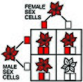 Outcomes of two sets of heterozygous red flowers, each with a one red and one white allele. Note that on average 75% of flowers will be red, and 25% will be white.
 -
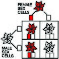 Outcomes of two sets of flowers one a homozygous white flower paired with a heterozygous red flower, half the flowers will be red, with one dominate red allele, and half will be white with two recessive white alleles.
 -
 Outcomes of two sets of flowers both homozygous white flowers because all the alleles are white and recessive, all the offspring flowers will also be white.
 -
![Outcomes of two sets of flowers both red. One red flower is heterozygous while the other is homozygous. All the offspring flowers will also be red, but some will carry the recessive white flower alleles.]]](//upload.wikimedia.org/wikipedia/commons/thumb/c/cc/Heterozygote-red-flower-homozygote-red-flower.jpg/120px-Heterozygote-red-flower-homozygote-red-flower.jpg) Outcomes of two sets of flowers both red. One red flower is heterozygous while the other is homozygous. All the offspring flowers will also be red, but some will carry the recessive white flower alleles.]]
Outcomes of two sets of flowers both red. One red flower is heterozygous while the other is homozygous. All the offspring flowers will also be red, but some will carry the recessive white flower alleles.]]


![Outcomes of two sets of flowers both red. One red flower is heterozygous while the other is homozygous. All the offspring flowers will also be red, but some will carry the recessive white flower alleles.]]](/wiki/File:Heterozygote-red-flower-homozygote-red-flower.jpg)
Imagine a deck of cards containing only red or white cards. Two cards are each dealt to each offspring pea plant player (we will call this hand of cards genotype) that will be used to determine the peas unique flower color (called a phenotype). The color will always be red, if any of the cards dealt are red. However, if the pea has no red cards, just white cards, then the plant will be white.
In this first game of cards (see above), the probability of a red card showing up is 75%, since the hand of cards could be two red cards (called homozygous since they are the same), one red and one white card (heterozygous since they are different), or one white and one red card (also heterozygous). All these hands of cards (called genotype) would result in a red flower.
The only way a flower would be white would be if the cards were both white (also homozygous). Hence red cards trump white cards in this game, and we referred these types of traits as being dominate. While white cards are recessive, meaning that you need both cards to be white in order for that trait to manifest white flowers as the phenotype. Each parent contributes one half of its cards (scientist called these hypothetical cards alleles), but only dominate traits are manifested when the pairs do not match, in this case red. This allows the diversity of traits to remain in following generations.

As a test, Mendel took pea plants of the first generation, white ones and pink ones, and self-fertilized them, so that they only drew alleles from themselves. The white peas only produced white flowers, because both cards were also white. However, pink peas produced both white and pink flowers in the subsequent generation, indicating that some offspring were heterozygous, containing both a pink and a white card (which again are called alleles, or heterozygous). Mendel did similar experiments with seven other traits with peas, ranging from the height of the plant, to seed shape and color, as well as pod shape and color. All appeared to be related to a key ratio or outcome that suggested a pairing of traits from unique alleles. Since inheritance appeared to be a probability distribution, variability within individuals can be preserved between generations, it is only the frequency of those traits that change. This discovery allowed the retention of variable traits that natural selection could work on. In 1863, Mendel read a German translation of Darwin’s Origin of Species book, which was all the discussion among a small group of scientists that regularly attended local meetings in Brno. Gregor Mendel in February and March of 1865 published his classic study, which he read before the Brno Natural History Society, and was published in 1866. The now classic study was never read by Darwin, and despite rumors of Mendel writing to Darwin during his lifetime, no evidence of correspondence exists between the two. Part of this lack of communication between the two scientists was likely a result of their differing languages, and the fact that Mendel was overly humble and fearful that his scientific experiments on peas would cast too much attention from those within the Catholic Church, who frowned upon his evolutionary experiments with plants. Mendel himself may have repressed his ambitions when he became abbot of the monastery in 1868, acknowledging his failures at the university, and avoiding attention to his scientific interests. Mendel’s ground-breaking research was to remain obscure to the greater scientific community, especially outside of Vienna, even among fellow botanists who could quickly understand the importance of his experiments.
Rediscovering Mendel’s Experiment

In 1886, the Dutch botanist Hugo de Vries collected primrose seeds and planted them in his garden, noticing the great variety of flowers that the seeds produced, it was from this observation that he speculated that the plants must exhibit spontaneous mutations between generations, with the continued introduction of new traits, or phenotypes. In fact, the word mutant was coined by de Vries himself. This idea, which helped to explain increased variation between generations, was built on an older idea that there was some mechanism that changes between generations. He termed this mechanism or unknown molecule, pangenes, from Darwin’s idea of pangenesis. Later scientists shortening this term to simply gene. Hence de Vries viewed that genes mutate between generations, which introduce variation between each generation, helping to solve Darwin’s dilemma with blended inheritance. The problem with this idea was that it contradicted the experiments conducted by Mendel on peas. Mendel’s experiments were also ignored by the Swiss botanist Carl Nägeli, who despite numerous correspondences with Gregor Mendel never mentioned his work in his own publications, however, one of his students, Carl Correns became aware of the experiments and retested them while at the University of Tübingen, his verification was published in 1900, using Gregor Mendel’s name in the title of his paper. Overnight Mendel’s experiment became well known in biology, revealing an apparent pattern in how traits are inherited from parent to offspring.
Chromosomes and the complexity of cellular division in Eukaryotes

Study of individual cells of eukaryotic organisms highlighted a complex process of cellular division, which invokes not only the copying of the nucleus of the cell, but also the many organelles within each cell. In bacteria, cellular division (called binary fission) is a simple process of DNA replication and cytokinesis, which divides the cell into two equal halves each containing a complete DNA molecule. In eukaryotic cells, cellular division is more complex, because the cell contains a nucleus in which sets of DNA are arranged into a series of chromosomes. Chromosomes in eukaryotes are held together by chromatin fibers, which prevent the long molecules from becoming entangled within the nucleus of the cell. Unlike prokaryotes, in which the DNA forms a ring or circle and floats in the cell freely, chromosomes in eukaryotes nucleus are extremely long tangles of DNA molecules paired into a series of rod-like chromosomes. During cellular replication in eukaryotes, the chromosomes condense such that they can be seen under a microscope, as tiny X shaped structures.
Mitosis

Most eukaryotic cells reproduce by mitosis. Mitosis is the cellular replication that results in two daughter cells each having the same number and kind of chromosomes as found in the parent nucleus. In multicellular organisms, mitosis cellular reproduction is responsible for ordinary tissue growth. Cells within a multicellular organism will continue to grow and be replaced through mitosis throughout the life of the organism, until all cells expire with death and no longer replicate. While mitosis in single celled eukaryote organisms produces two copies (or clones) of the cell, with nearly identical copies (asexual reproduction).
There are a number of stages in mitosis cellular division in eukaryotic cells, the end result of which is that each chromosome is paired up (Prophase,) hung on a mitotic spindle (Metaphase), and then pulled apart into individual chromatids (Anaphase), replicating the missing paired chromosome to form a new nucleus (Telophase), and finally the cell will pitch off in the middle (Cytokinesis) forming a new copy of the parent cell. This type of replication is occurring all the time in multicellular organisms, producing new tissue and growth over time. This cellular replication allows a multicellular organism to heal and repair itself, and is happening throughout your body right now. Single celled eukaryotic organisms mitosis is a method of asexual reproduction. Each cell produced during mitosis is said to be a diploid (meaning that each cell has two copies of each chromosome).
Meiosis

The other type of cellular reproduction is called meiosis. Meiosis is much rarer, and only occurs in sperm and egg cells, called gametes in multicellular organisms. These cells rather than being identical copies of the original parent cell, produce genetically unique cells. First the cells produce four genetically unique gamete cells, each with half the number of chromosomes as found in the parent cell (haploid cells). These cells then come together through sexual reproduction between individuals. This process shuffles the genes forming new pairs, one received from each parent gamete cell, producing recombinant chromosomes with unique genetic combinations.
The best way to think of meiosis is that it is like shuffling two decks of cards (one from each parent) and splitting each deck to make a total of four piles, and then combining two of the piles to make a new deck with the same number of cards. In many primitive multicellular plants (such as ferns and many alga), these gamete cells can form gametophytes, or multicellular individual plants that contain only haploid cells. This results in a strange life cycle that starts with meiosis by reducing the number of chromosomes in each cell by half to make abundant haploid spores. These spores are released to the environment and develop into a gametophyte. The mature gametophyte produces male or female gametes (or sometimes both) by mitosis. These male and female gametophytes then come together in the water to produces a complete diploid zygote/seed (a cell with paired chromosomes). The fertilized seed then develops into a new sporophyte that will produce haploid spores and start the process again. Most gametophytes are small and associated with only the reproductive stage of a life span. Spores on the other hand can be protected for long periods of time (such as dinoflagellate cysts), and only become active when conditions become ideal for the organism to reproduce. Such a life cycle is employed by dinoflagellates, which are single celled eukaryotic organisms that make up much of the Earth’s phytoplankton in the oceans. Dinoflagellates, when they bloom during ideal conditions can result in toxic red tides for fish and other animals in the oceans. These organisms have evolved these strategies to help them survive harsh natural conditions.
Genetics
The discovery of how variation is maintained in a population of individual life forms through the continued recombination of chromosomes has revolutionized science. Many diseases and traits are inherited through genetic material either directly by recessive traits or by incorrectly copying chromosomes (such as chromosome duplications), or by mistakes or mutations that result in maladapted cells during cellular reproduction, such as in cancer. A clear overview of genetics is beyond the goal of this class, but knowledge of its existence explains the wide variety of life on Earth.
The Importance of Population Size and Genetic Diversity
One of the important factors that leads to new varieties of life on Earth is something called the founder effect. The founder effect is the loss of genetic variation that occurs when small populations are isolated. These small samplings from the larger population will statistically be limited in their genetic variation. This will cause them to exhibit fixed states due to the random sampling of the original larger population. This can sometimes be caused by a population bottleneck, when populations drop to small numbers. These tiny populations may not genetically represent the original population by their characteristics, and over time become unique, with increased inbreeding, and low variation. These isolated populations might become new species, but they are also prone to extinction. New species often originate from such isolated pockets in a geographically distributed population.
| Previous | Current | Next |
|---|---|---|
7g. Earth’s Biomes and Communities.
Biogeography

The best way to study the Earth is to travel. The study of the numerous varieties of life-forms on Earth is only appreciated when one travels across the surface, and notes the differences they see on their journey among the plants and animals they witness. Hence the study of life on Earth is linked to the physical geography of the planet in respect to the occurrence of different plants and animals, and the physical environment that they live within. This is largely due to specific adaptions that organisms exhibit to deal with the physical environment of each region. Hence, life in the dry deserts will exhibit different types of animals and plants than cold polar regions, while hot lush rain forests will exhibit a different diverse group of plants and animals unique to each region. The study of the geography of life is the fascinating field of biogeography.

The study of biogeography likely has its origins in the work of Alexander von Humboldt, a wealthy German explorer who lived 200 years ago. Alexander von Humboldt hope to travel the world, but the raging Napoleonic wars in Europe had caused travel to be difficult, both for funds and permission to travel across warring nations. He had hoped to join a research ship to journey around the world, but the war caused the voyage to be canceled. He requested to join Napoleon Bonaparte in Egypt, but the French authorities in the army refused to bring him along. In 1799, Humboldt’s luck changed when Charles IV of Spain authorized his travel of the Americas. Between 1799 to 1804 Humboldt traveled across South and North America and wrote about the experience in his detailed scientific notes. When he arrived in the United States in 1804, he was summoned by Thomas Jefferson at the White House. Jefferson had just completed the Louisiana Purchase from France but knew little of the regional geography. He was eager to consult Humboldt. Humboldt had traveled extensively in Mexico, although his travel into the interior was somewhat limited, they both shared an interest in the animals and plants that might exist in these unexplored regions. The work of Humboldt had a major influence on the idea of nature; indeed biographer Andrea Wulf attributes Alexander von Humboldt as the inventor of the modern notion of nature itself (see Wulf, 2016). Humboldt and many of his age viewed two worlds on Earth, first the world of man containing farms and urban centers in the cities and towns and second the world of nature, the wild and unexplored regions of the Earth. This two-world view of Earth is still prevalent in the modern age. The primary reason for these early explorations funded by governments, was that plants and particularly the raw production of goods from those plants, such as cotton, sugar, coffee, tea, and various crops, were becoming increasingly in demand by growing populations. The discovery of tomatoes, potatoes and corn in the Americas made these early botanic explorations highly lucrative, particularly for the European monarchies that oversaw these colonies in the Americas.
There was intense interest in understanding the distributions of plants and animals on Earth, as they were viewed as an important raw resource, from furs brought back by trappers and timber from lumbermen to food and exotic spices. Biological exploration was tied to understanding the major biomes of the planet particularly during the years of colonization. A biome is a distinct biological community of plants and animals that have formed in response to a shared physical climate. Early geographers of the distribution of plants on Earth, such as the Danish naturalist Fredrick Schouw, provided early classifications of these various regions. Botanists like Franz Meyen in the 1830s were well aware that the local climate, and in particular the average and extreme temperatures and amount of moisture, were very important to explain the unique distributions of various species of plants and animals on Earth. The concept of zones or isotherms, using Humboldt’s term, are areas of similar climates, and hence tend to produce similar plant and animal species. Most important, these zones could dictate which types of plants and animal can be grown in each region of Earth.

The history of sugar cane is an excellent case as to the importance of understanding biomes. Sugar cane, which is today a major source of sugar, originated in New Guinea, and was introduced into Southeastern Asia. The plant was then introduced to parts of the Middle East, but because of the dry climate, did not grow particularly well. Sugar was a rare medicine for much of Europe, and only eaten on rare occasions. With the discovery of the Americas in 1492 by Europeans, it was quickly recognized that the wetter and warmer climate of the Caribbean Islands and South America would be equally suitable for growing and harvesting sugar cane. The earliest sugar plantations were first established as far back as the early 1500s, and with the rapid rise of sugar cane in the New World, it became a very common import into Europe and across the Americas, particularly in places too cold for sugar cane to be grown. This shift resulted in the enslavement of millions of people, particularly from Africa for the continued harvest and cultivation of this plant in the Americas. Soon people in Europe where consuming sugar at much higher levels than ever before, with great demand for sugar in places where it was too cold for the plants to grow. Early biomes were mostly defined on a general description of the local climate, such as deserts, polar regions, or wet tropics, but others defined them based on particular types of plants that grow within them. For example, palm trees, sage brush, or cactus regions on maps.
In the 1860s, Wladimir Köppen traveled frequently on the newly constructed train from his family’s home in the warm southern Crimean city of Simferopol to the far cold north city of Saint Petersburg in northern Russia. The train journey of 2,110 kilometers (1,305 miles) is a nearly direct north-south transit across eastern Europe crossing many different climatic regions along the way. During the journey he would watch from the train the slow changes that occurred among the plant communities that he saw out the window, as they crossed each particular climatic zone. Later in his life, he would use the experience to develop the Köppen climate classification that was first introduced in 1884, and has been modified over the years into a geographic map of Earth that classifies the geographic zones of each of the major terrestrial biomes of the Earth. It is today referred to as the Köppen-Geiger climate classification based on improvements made by Ruldolf Geiger.

.jpg)
The map is a precursor to the United States USDA Plant Hardiness Zone Map that has become in standard use by gardeners and farmers in the United States to determine if a particular plant species would be successfully grown in their garden, depending on the average climate of that region. For example, the state of Utah spans zones 9 through 4, with the southern city of Saint George within the warmer 9 and 8 growing zones, while Salt Lake City is within the 7 and 6 growing zones, and the higher elevation and cooler and drier cities like Vernal and Heber being within the 5 and 4 growing zones. Each zone is demarcated by the average annual minimum winter temperature, divided into 10-degree zones. Unlike the Köppen-Geiger climate classification system, the USDA Plant Hardiness Zone Map is based only on temperature, rather than a combination of temperature and moisture. Both maps and classifications must be updated as each region’s climate changes over time. Furthermore, both classification systems are based on the climate, rather than the occurrence of plants and animals. Other classifications have used the types of soils found in each region to demarcate each biome based on the soil type found in the area. These of course only describe the major biomes of Earth’s terrestrial ecosystems, leaving out the various ecosystems of the Earth’s oceans, which are related to other physical conditions such as salinity, water temperature, light and water depth. These biomes describe the physical abiotic environment and don’t define them on the occurrence of plants or animals as part of their definitions. For example, such systems would not recognize altered environments or biomes, such as agricultural lands and urban city centers that have been heavily altered by human intervention, yet may have similar climatic conditions as naturally preserved lands that are protected.

Beginning in the 1970s the botanist David Goodall lead a team of biologists, ecologists, conservationists and land managers to summarize the major biomes on planet Earth in a multivolume book series, entitled Ecosystems of the World. They defined 30 major biomes on Earth, including biomes rarely defined in other systems or classifications, for example subterranean biomes like those found in caves. The Goodall’s classification also divided the Earth into natural biomes from those of human or managed biomes, such as field crops, managed grasslands and industrial urban landscapes. Hence two theories emerge on how to classify the major regions of Earth into biomes, one that is based on the occurrence of living organisms and one relies on the physical climate.
Support for the inclusion of specific biological species in the biome classification system comes from the central idea of keystone species. Keystone species are biological species within an environment that disproportionately affect a large number of other species in the same environment, and their removal from the region would completely alter the entire ecosystem drastically. A keystone species is sometimes not the most abundant, but one that influences the ecosystem the most and helps to maintain it. For example, many apex predators like wolves and lions are often considered a keystone species, because they have a significantly large influence on the occurrence of prey, as well as the plants that those prey animals might depend on.
Although many biomes are simply defined by the basis of the most abundant species, or the species with the largest amount of biomass in the environment. Biomass is the total mass of a particular species of organisms in a given area or volume. For example, the grassland biomes are defined by the large amount of grass plants that live within the region, while conifer forest biomes are defined by the large amount of biomass of conifer and pine trees. Hence biomes can be defined based on the most abundant and common of the biological organisms within a particular region on Earth.
The Major Biomes of Earth
There are many ways in which the Earth has been divided into major biomes. This list is not comprehensive, but includes most of the major biomes that are widely distributed on Earth, and easily recognized by the occurrence of species and climatic and physical conditions found within them.
Terrestrial Biomes
Tundra Biome
.JPG)

The tundra biome occurs at high latitudes near the north and south pole, and represents cold regions on Earth, which are also some of the driest regions on Earth. In these regions the soils are frozen throughout the year as permafrost, with only a thin melt during the height of the summer. These soils are very ancient with only minor yearly growth of lichens and other arctic plants. The very short growing season and low light levels during the winter result in low species richness. The landscape is dominated by lichens and mosses, with grasses and other low laying plants adapted to the cold. Many migratory animals live in these regions of Earth including birds and caribou, as well as polar bears, that often move great distances across the landscape.
Boreal Forest Biome
.jpeg)

The great taiga or boreal forests span much the upper latitudes of Canada and Russia. The boreal forest is dominated by cold winters and short growing seasons, with a forest of mostly coniferous trees, which remain green through the long winters. Conifers are a group of trees (gymnosperms) that evolved early in Earth’s history, bearing cones and wind-blown pollen, rather than bearing flowers and fruit. They are perfectly adapted to these seasonally cold regions of Earth, allowing their wind-blown pollen and cone bearing seeds to germinate in the cooler climates. The region contains many mammals, such as wolves, foxes, rabbits, moose, deer, and bison, but fewer reptiles like lizards, snakes and crocodiles, due to the cold climate.
Alpine Biome


The alpine biome is sometimes included in the boreal and tundra biomes depending on the elevation of the landscape. These are topographically high regions on Earth that are also seasonally cold, due to their high elevation. Increasing altitude on Earth decreases the average yearly temperatures, resulting in a similar profile as observed with the higher latitude tundra and boreal biomes. Alpine biomes are unique in that they are isolated on these alpine peaks and plateaus, and while having a similar climate to tundra and boreal regions of Earth they are unique in their isolation. Some alpine biome regions like the Himalayan Plateau are fairly extensive. One important aspect of the alpine biome is called the tree line. The tree line or timberline is the upper boundary of forests on a mountain peak, above which trees are unable to survive. This elevation varies between 10,000 feet (3.0 Km) to 12,000 feet (3.7 Km) above sea level across the United States, and depends on the amount of moisture and annual temperatures, but the tree line can be much lower in elevation the closer one travels toward the poles (higher latitude) as the climate becomes colder in these regions. These mountain top regions are often covered in ice and snow, both as semi-permanent glaciers as well as winter snow and ice that remains long into the summer months.
Temperate Rain Forest Biome


Temperate rain forests are found in the pacific northwestern coast of North America and South Eastern Australia, which are characterized by higher levels of moisture along these coastal regions. They often are filled with large evergreen trees including some of the largest trees that grow on Earth today. The heavy rain, and somewhat milder climate results in a lush forest landscape and hosts many plants that need high levels of moisture to survive including ferns and horsetails. They also host many epiphytes. These are plants that live on other plants like orchids, vines, ferns and moss. These biomes have a high diversity of amphibians, as well mammals and birds when compared to colder and drier biomes. These biomes are a major source of lumber, and affected by industrial forestry.
Temperate Deciduous Forest Biome


This biome includes large regions of the eastern United States, most of northern Europe, and Eastern China, where the climate alternates between mild winters and warm summers, with a fair amount of rain and snow. Temperate deciduous forests are characterized by trees that have adapted to the seasonal changes by losing their leaves in the fall, and re-growing them each year during the spring. This prevents the branches from breaking with the weight of snow in the winter months, but also allowing a greater surface area for photosynthesis in the warmer summer months. These forests are dominated by maple, oak, birch, and elm trees supported by rich soils. These regions are often cleared for farms and agriculture and host major urban centers because of the biological productivity of the soils for growing crops. Temperate deciduous forest are likely more dominate in Earth’s past, but have changed their distribution as the Earth has undergone various glacial and interglacial periods during the last several ice ages.
Tropical Rain Forest Biome


Tropical rain forest biomes are the most species rich biomes on Earth, and exhibit an enormous amount of different species of both plants and animals. This is a result of the lack of seasons, and the continued large amounts of rainfall. Tropical rain forests occur on land below the atmospheric Intertropical Convergence Zone (ITCZ), in which rain nearly continuously falls due to the atmospheric circulation and low pressure as a result of the equatorial position of these forests. This stable warm and wet climate allows trees to remain green throughout the year, and grow much more slowly. This also means that the forest is not shedding significantly large amounts of biomass onto the forest floor like in temperate deciduous forest, and the soils are organically poor, often sandy and leached of nutrients by the abundance of rain. Tropical rain forests support a tall forest canopy that is enclosed year-round, making the forest floor particularly dark. Closed forest canopies prevent sunlight from reaching the forest floor, while open forest canopies, where the trees are more widespread allow more sunlight to reach the forest floor. In close canopy tropical rainforests, sunlight is the limiting resource for plants. Tropical rainforests exhibit poor soils, and when cleared for agriculture often lead to muddy or sandy barren regions of dirt, since the soil is lacking organic carbon molecules and nutrients for plants to re-establish themselves. The rapid deforestation of rain forests has led to significant changes to these biomes, including the occurrence of forest fires. Forest fires in tropical rainforests result when famers and industrial agricultural agents clear the land. The cut wood is stacked and dried, and often set on fire to remove from it, but even if the wood is harvested or clear cut from the forest and removed by trucks, and the waste of wood shavings, chips, branches, twigs and saw dust is burned in large piles. These fires can set the surrounding virgin forest on fire, especially when they blow into these parts of the forest. Over the last decade there has been significant destruction of the tropical rainforest biome. In August of 2019 an estimated 3,500 square miles, or 9,060 square kilometers of the Amazon forest burned in fires across Brazil, Paraguay and Bolivia.
Tropical Deciduous Forest Biome


Tropical deciduous forests are characterized by seasonal wet and dry seasons, within warmer or tropical climates. These are sometimes referred as monsoon forests, as they are influenced by changes in the amount of rainfall. The forests across India, as well as Southeastern Asia, and parts of South America and Africa are greatly influenced by these cycles of rain. These regions rarely if ever see snow, as their temperatures remain warm throughout the year. A result of the monsoon cycle is that the soils often are red in color, due to the oxidation of iron, and tend to be less rich in nutrients than temperature deciduous forests because of leaching. Trees go dominate during the dry seasons and have a specific growing season.
Grassland Biome


Grasslands are broad regions of prairie or grassland steppes that lack significant numbers of trees due to the lack of water. They often have temperate climates, with cold winters and warm summers, and host a wide diversity of grass plants and other low laying scrubs. Grasslands undergo intense growing seasons in the summer, and fall dominate in the colder winters, leading to rich soils, despite the lack of trees. Grasslands host large mammals that feed on the grass covered landscape, including bison and prong horn antelope here in North America, but also have abundant insect and rodent populations, as well as snakes and lizards. Much of the world’s grassland biomes has been replaced by either grazing land or agricultural farms for the growth of wheat and corn. A few protected areas remain, established after the Dust Bowl years in the 1930s, the United State Government established national grasslands although much of this land is open to be leased for cattle, but are protected from agriculture to help maintain the soil.
Grazing Land Biome


Land that hosts large numbers of cattle, sheep, goats and horses for grazing is this biome, which incorporates aspects of grassland, savanna and desert biomes, but could include cleared forest land. Much of the grazing land biome is privately owned as small fenced fields to large ranches, but also includes government managed land that is leased to ranchers for access to grazing. Both cattle and sheep have been introduced to these areas, where they are raised for their skins and wool, as well as for their meat around the world. Grazing land depends on a rich source of grass vegetation, and often cultivate invasive species of plants such alfalfa or lucerne (Medicago sativa), cheat grass (Bromus tectorum) and knapweed (Centaurea diffusa).
Agricultural Biome


The agricultural is the biome of farms and irrigated lands that grow any type of crop. Often these are in regions that have a source of water that can be used on the crops to increase the growth. They typically have very low species richness and biodiversity of any biome because of the heavy use of pesticides and other deterrents for pests that might eat the crops. Corn, wheat, rice, and hay are the major crops on agricultural lands, incorporating various climates from wet rice paddies to dry wheat or alfalfa fields. Agricultural land covers much of the habitable terrestrial land on Earth, and relies on healthy soils and sources of water for the continued growth of food. It can host various mammals and birds, but often has limited biodiversity in plant life, which is found on the periphery of the biome.
Savanna Biome


Savannas are a mix of grassland and forest, which are composed of a scattered distribution of trees. They tend to have high temperatures, and more drier climates, with very seasonal rainy seasons. Savanna biomes are found across the African Sahel in northern Africa, and extending into Southern Africa, both places where precipitation is much lower than the more tropical equatorial regions. Savannas are biologically diverse, supporting large herds of mammals, and host animals from elephants, lions, zebras, antelope and wildebeests.
Chaparral Biome

Chaparrals are very dry biomes that support low scrubby evergreen bushes, and short drought-resistant trees. They are found in Southern California, parts of Arizonia, as well as around the Mediterranean Sea and Middle East and parts of Australia. A result of the vulnerably to frequent droughts, the chaparral biome is affected by frequent wild fires. Plants also tend to have large root structures that can tap into sources of water deep underground, and re-establish themselves after fires.
Desert Biome


Deserts are regions with low-precipitation and temperate to extremely hot climates. As arid environments, deserts have less total biomass, and depend on infrequent rain or snow. Plants are often adapted to the low availability of water, with some deserts nearly lacking plants altogether, with the landscape covered by blowing sand dunes. Many types of deserts exist, in Utah, the desert is a continental interior desert, in that low precipitation is due to the rain shadow of the more coastal mountain ranges in Nevada and California, which prevents significant rain compared to the coasts. Located within the center of the continent, these regions exhibit more extreme warm or hot summers, without the heat sink of the ocean. Deserts are found along the narrow strip of land between 30 to 40 degrees latitude, which due to the Hadley Cell atmospheric circulation pattern are under high pressure most of the time, and tend to exhibit dry air descending at these latitudes. This push of high pressure across these regions on Earth leads to air with low humidity and is undersaturated in respect to the availability of water. As the Earth warms the extent of Earth’s desert biomes is expect to expand poleward, as the atmosphere increases in temperature, leading to increased risk of drought in higher latitudes.
Cave Biome

Cave biomes are the unique life that lives underground in caves. Exhibiting a low species richness and diversity, caves offer a unique biome for life to live outside of the light, and utilized the cave temporarily as shelter. Cave biomes are interesting places to study the unique microscopic and bacterial life forms that are able to live in a biome without light. They often utilize sources of nutrients brought into caves, from such creatures as bats and small mammals that seek them out for shelter.
Urban Biome

.jpg)
The urban biome is likely the one that you are most familiar with since it encapsulates much of the landscape within city and town centers where most people live. This biome includes roads, parks, gardens, golf-courses, parking lots, homes, shopping centers, and warehouses. It is dominated by cultivated plants interspersed with asphalt roads and concrete sidewalks, with structures and buildings. They tend to have a higher biodiversity than agriculture lands due to the cultivation of a wider range of plant species, but like agricultural lands often relies on irrigation. The urban biome is home to many domesticated animals, such as cats and dogs, as well as humans, but also are frequented by raccoons, rats, and mice. The urban biome is rapidly expanding as new housing developments are built, which often grow out into the surrounding biomes. Urban biomes have high levels of plastic waste and other types of human refuse.
Aquatic Biomes
Freshwater River and Creek Biome


Rivers, streams and creeks and flowing freshwater on Earth are an important biome for both aquatic fish and insects, as well as the animals and plants that use these as sources of water. Flowing freshwater is an important source of well oxygenated waters that are utilized as spawning grounds for migratory fish. Large standing water bodies of water are prone to lose oxygen, especially in warm climates, and the flowing nature of freshwater rivers and streams provide an important biome for fish and the animals that depend them for food. Rivers provide a biome that is complex, as these ribbons of water move across different climates and elevations offering a path toward the interior of continents for aquatic life, as well as plants and animals that need access to water. The study of the freshwater river biome or ecosystem is called limnology.
Freshwater Lake and Pond Biome

Freshwater lakes and ponds are equally important biome of the freshwater system and interconnect rivers and streams. Lakes and ponds are biologically rich areas for supporting both aquatic animals and plants, as well as animals and plants that depend on them as a source of water. Many plants live in the shallow littoral zone on the edge of lakes including cattails, horsetails, and reeds. These regions are important for migrating birds, such as ducks and other waterfowl. Just like the ocean, lakes can become stratified, and can lose oxygen through eutrophication. Such events result in the death of fish and other animals that rely on well oxygenated waters. These events mark episodes of major disturbances to the biome, which can also occur during droughts as water levels drop, decreasing the extent of the biome.
Wetlands, Swamps and Marshes Biome

Wetlands are broadly defined as any land that is wet or covered by water during any part of the annual season. Mostly they are found in low poorly drained basins, where water will accumulate during rainy seasons. The amount of water and its depth various, but this more ephemeral source of water is important for amphibian, crocodilians and snakes, as well as birds and mammals. Trees often grow within these damp biomes, such as bald cypress (Taxodium distichum), that can live in standing water found in swamps in the southeastern United States. Many wetlands have been drained for use of the water, and various governmental agencies have worked hard to protect this biome.
Estuaries, Deltas and Tidal Flats Biome

This is a transitional environment between the ocean and land, and connects rivers and freshwater sources of water with saline ocean waters. This produces a biome similar to swamps and marshes, but with the water having a mix of salinity. These biomes are influenced by the daily and monthly tides, as well as longer term rise and fall of sea levels, which can flood regions along the coast. These regions are held together often by mangrove forests, which help trap sediment and nutrients, but can tolerate the salty water. Many invertebrate animals make use of the tides and water by burrowing into the muddy substrate, and filter feeding as the water moves in and out during the tidal cycles. Bivalves (such as clams and mussels) and barnacles as well as bryozoans, often encrust the rocks and wood to filter out food from the water. They are important biomes for birds, crocodilians, turtles as well as fish.
Coastal Lines and Beaches Biome
.jpg)
Beaches are also referred to as the littoral zone of the ocean, as it includes both the sandy coastline as well as the shallow near shore. The breaking of waves, and everchanging tides make beaches an interesting biome for animals and plants. Kelp (or seaweed) of the brown algae class Phaeophyceae, grows in the water, buoyed up by air sacs that help keep the kelp floating within the photic zone. Echinoderms, such as starfish and sea cucumbers lives in this zone, as well as gastropods (snails). Other mollusks such as bivalves dig down into the sandy substrate to filter feed from the passing water. The high energy of the beach coast line and crashing waves, make this region a seemly constantly changing environment, but it is rather stable over time when compared other biomes.
Open Ocean (Pelagic zones) Biome

This is the open ocean biome of swimming and floating plants and animals. The pelagic zone is divided into the photic zone near the surface, and the deeper aphotic zone below, which is dark. Animals live within this zone by freely swimming (like fish, sharks, and marine mammals and various invertebrates (like shrimp and cuttlefish), and those animals that float in the water (jellyfish, plankton, such as tiny dinoflagellates, diatoms, and foraminifera). The Open Ocean Biome is the largest biome on Earth and covers the most volume on Earth. This large volume is because the open ocean or pelagic zone includes a wide range of depth within the ocean waters. This biome is also the least visited by humans, and remains poorly understood given the challenges of studying these ocean creatures.
Ocean Floor (Benthic zones) Biome

The finally biome is the ocean floor, the animals that live by crawling around or sessile (attached to the ocean floor). The benthic zone covers about 70% of Earth, and host a wide variety of biomes, from near shore coral reefs, lagoons, to deep abyssal and hadal zones in the deepest and darkest parts of the Earth. The ocean floor is a unique biome because it depends heavily on the input for organic nutrients from the pelagic zone above, and much of the ocean floor lacks access to sunlight for energy. Most of the organisms that live on the ocean floor utilize the organic waste that rains down, making most of these organisms scavengers or decomposers with them utilizing chemosynthesis.
Measuring Biodiversity
Biodiversity today is often defined by the total variety and variability of life on Earth. It is often used in discussions of its importance for the preservation and protection of key biomes on Earth that support the many biological species. In measuring biodiversity ecologists define two indexes that can be used to compare biomes or regions. The first is richness.
Species richness
.jpg)
Species richness is simply the number of species that have been documented in a certain region or area, while family richness is defined more broadly as the number of families or closely related groups of species in a region or area. Species richness is determined by counting the number of different species within a geographic region, from a single country, or county to a broader ecosystem or biome. The various biomes on Earth have varying degrees of species richness. Tropical rain forest biomes of the Amazon and Congo Rainforests contain very high species richness, with nearly 20,000 species of vertebrates in these areas, while tundra and boreal forests biomes near the poles have low species richness with about 1,000 or less species of vertebrates. The cold and open tundra biome contains less resources for food and shelter, and a harsh environment for biological species. The complexity of the tropical forest environment and uniform climate allows for numerous environmental resources and a stable environment to live in. Species richness is correlates to latitude, with low latitude, equatorial regions having high species richness, while high latitude polar regions having low species richness. Moisture, and the average annual rainfall also effects species richness, but less than the variability of the season temperatures. In the ocean’s warm coral reefs, lagoons and estuaries all exhibit high species richness, while dark cold deep ocean water and regions with high salinity exhibit low species richness, due to limitation of resources within these regions of Earth.
One observation is that animals that live near the poles at high latitudes tend to be larger than animals that live near the equator. This is referred to as Bergman’s rule, named after Carl Bergman, a German a professor of anatomy and physiology in the mid-1800s. One explanation for this pattern is physiological, animals that live in colder climates will be larger to maintain body temperature during colder months of the year (low surface to body ratio), while warmer climates will favor smaller animals that are able to disperse heat more effectively with high surface to body ratios. This applies only to endothermic animals, like mammals and birds.
Determining species richness requires numerous surveys in which each organism is identified to its unique species. This is in practice is difficult to accomplish, although various government agencies have supported such efforts, often relying on the volunteer work of experts in various groups of organisms, from botanist, entomologists, herpetologist, ornithologists, and mammologists, each identifying the species in a given area. Species richness relies on a statistical process called rarefication. For example, each time you visit an area there may be different numbers of species present and observed. Rarefication is the continued sampling of individual organisms and measuring the likelihood of a new and novel species being counted. It looks at the curve of the increasing number of species, and how likely a new species will be encountered on a subsequent visit to the area. This is important, because many species are rare or only visit the region at certain times of the year. Another challenge in studying species richness is that many species, such as microscopic life, are often overlooked in such surveys. It is likely that many biomes are much richer in biological species than currently understood.
Biological diversity
Biological diversity is a measure of the representative abundances of each species in an environment. A biological diverse environment will have more species, but also a more evenly distributed abundance of these species in that environment. One of the measurements to determine biological diversity is the Shannon-Wiener index.

Let us use a simple example of two groups and compare their Shannon-Wiener index using this formula above. One environment contains the following species:
- Survey One
- Species A = 25 individuals
- Species B = 3 individuals
- Species C = 1 individuals
- Species D = 2 individuals
- Species E = 3 individuals
Here we have 5 species represented by 34 individuals. First, we calculate the proportion of each species by dividing the number of individuals of that species with the total number to get proportions, for example Species A has 25 individuals out of 34, so it represents a proportion of 73.5% in the environment, while Species A with a single individual only represents 1.03% of the individuals. We take the natural log of each of these proportions, multiple them by the proportions, and total them up, divide by the number of species to get a mean and take the negative of the resulting index. So, for this first group the Shannon-Wiener index diversity is 0.185. Let us look at a second group.
- Survey Two
- Species A = 3 individuals
- Species B = 3 individuals
- Species C = 3 individuals
- Species D = 3 individuals
- Species E = 3 individuals
Notice in this group has 5 species, so the species richness is the same between these two groups, but now we have only 15 individuals, but each of those have similar proportions of 3.
.jpg)
.jpg)
We take the proportion of each of these species, which are all 32% and take the natural log, and multiply the result by the proportion, and take the mean by dividing the total by 5, then take the negative. In this cause the resulting index is higher 0.322. That is because there is a more equal proportion of each species abundance to each other. We can say that the first group is less diverse than the second group, despite the fact that there are more individuals in the first group. Such measures of biodiversity are very important because a single species can come to dominate a region, this is particularly an issue with invading species and in particular agricultural and grazing lands where plants or animals of a certain type predominate at the expense of other species. This process results in very low biodiversity in these regions, and often is reflected in species richness numbers as well.
One of the central issues in the study of biodiversity is understanding the mechanisms for promoting a biological diverse ecosystem and maintaining it. Both ecological and paleoecologically studies suggest two major factors come into play in maintaining a biological diverse biome. First is a stable physical environment, with a climate remaining seasonally stable for long periods of time, and second that the environment is left undisturbed, avoiding short term events such forest fires, asteroid impacts, urban and industrial development and other short-term calamities that result in an alteration to the landscape. One aspect of disturbing a landscape is the introduction of a rapidly reproducing invasive species, which can take over a region and dominate the biodiversity of the area. But most disturbances to the landscape are done by humans directly, from building a road, to plowing a field.
Ecological Succession


Ecological succession is the process under which biological communities of plants and animals recover from a major disturbance. These disturbances can be natural, like landslides, volcanic eruptions, or wildfires, or be human induced such as clearing a forest for agriculture, mining, or industrialization of the landscape such as oil and gas drilling, building a parking lot or road and driving across the land. All these disturbances leave behind major altered biological communities, often with highly reduced species richness and biodiversity than before the disturbance. Ecologists study how long an area recovers from a particular disturbance. Ecologist begin by defining a Climax Community. A climax community is a stable community that is self-perpetuating and in equilibrium with the physical habitat of the area, with high levels of species richness and biodiversity, with low to no decline of species occurrences within the area. A climax community can be regarded as a stable community with high biodiversity, that would have existed prior to the disturbance. Early naturalists, like Henry David Thoreau wrote about the succession of forest trees from farms that had been cleared, but subsequently left fallow, and were eventually replaced by trees that reclaimed the farm field after numerous years had passed. One of the key scientists in the study of ecological succession, who also helped coined the term ecology, was Henry Chandler Cowles. In the late 1800 he studied areas that were covered by wind-blown sand dunes and studied how plants re-established themselves over the course of multiple years. Volcanic eruptions and intense wild fires have also proven interesting case studies to understand the succession of plants following the recovery of disturbance.
The idea of ecological succession governs much of land management practices, particularly in the United States where land disturbance is widely regarded as transitory and temporary, and given enough time, the area will recover to its pre-disturbance state. However, land disturbance by human activities often are not a rare occurrence, but frequent, cyclic and cumulative over time, limiting the full recovery. Often a prior climax community may be unknown, as the area may historically have been over grazed and clear cut to begin with. With frequent ground disturbances over hundreds of years, the original species richness and biodiversity of the area may not have been recorded prior to the initiation of these disturbances. Disturbed areas are susceptible to invasive species of both plants and animals, often which take a foothold into the area and alter the area differently than prior to the disturbance. Land managers may alter the environment on a continued basis, such the massive removal of juniper and pinyon trees across Utah to provide grazing land for cattle on public lands or efforts to start controlled burns to prevent major wildfires that might destroy economical valuable structures. Reseeding programs, where disturbed lands from mining and oil and gas drilling on public lands are re-seeded lead to different replacement vegetation, as those that existed prior to the ground disturbances. Contamination of ground water, or the draining of ponds and lakes for use on crops, can lead to long term changes to the land, altering the availability of water making a succession toward a climax community not likely. Furthermore, a consequence of a changing climate over time, and the long-term process of ecological succession, means that prior climax communities existed under a cooler wetter climate, and these plants and animals can no longer be established in the area because of climate change. In truth, the concept of Earth’s biomes is in flux, and changing, with examples of natural biomes becoming limited to protected lands on national parks, and a growing expanse of disturbed lands (such as Urban, Agricultural, and Grazing Biomes), within new sets of biome definitions.
| Previous | Current | Next |
|---|---|---|
7h. Soil: Living Dirt.
Living Dirt
Earth is the only planet with soil. As truly defined, soil is the ecological biome that exists in the shallow subsurface on Earth and includes both living and dead organisms, as well as the natural mineral and rock resources that sustain the living biota within and above the shallow terrestrial subsurface of Earth. Soils are important for the terrestrial organisms that rely on the nutrients, moisture and substrate that provide attachment for plants, fungus, and bacteria through their extensive roots and distribution through this narrow horizon below Earth’s surface. Eroded rocks and minerals, lacking significant organic contain, like that found on other planets is called regolith. Regolith is the covering of unconsolidated dust, broken rocks, and various minerals that cover the deeper bedrock of a planet, and is found on Mars and the Moon. Soil on the other hand, which is unique to Earth, contains abundant organic material, both living and dead, such as decaying leaves, organic compost, bacteria, invertebrates, such as annelid worms, complex roots, fungal molds and burrows of animals. Hence, soil is part of Earth’s living biome.
Typical Soil Horizons

All soils exhibit a set of horizons which are identified by combination of leaching due to the precipitation of rain or snow melt moving into the soil subsurface and carrying dissolved ions deeper, while also the continued input of organic dead vegetation (leaves and other plant litter) and transported sediments onto the surface. Through these natural processes, soils develop a set of characteristic horizons. These soil horizons were codified by Russian soil scientist Vasily Dokuchaev. In the 1890s, Vaily Dokuchaev was commissioned to study soils around the Russian city of Nizhniy Novgorod. The city is located at the junction of the Oka River and Volga River, within the agricultural center of the Volga drainage basin that provides even today much of the world’s wheat. Soils and their study was important to continue the projection of crops in the region, and Vaily Dokuchaev codified soil horizons into a set of four major horizons.
O Horizon- The O horizon is the organic rich horizon at the top at the atmosphere-geosphere interface, between the gas filled part of Earth and the solid interior. It is called the O horizon because of the abundance of organic matter. Most of this organic matter is living and dead plants, but also includes living and dead bacterial, fungal and animal matter. The O horizon varies in thickness, sometimes its absence or paucity in certain biomes like desert and tundra environments. In other environments the O Horizon can be thick, especially when there is a supply of organic matter such as temperate deciduous biomes, where trees lose their leaves in the winters, and temperate grasslands, which go dormant during the winter months, adding organic matter to the surface of the soil, which gets buried over time. This horizon is nutrient-rich, and tends to be strongly humified with moisture retention.
A Horizon- The A horizon is a mixed horizon, with the cumulation of organic matter from above and the process of weathering, with the input of wind-blown dust that produces an organic and clay-rich zone. The A horizon is subjected to bioturbation, the process of burrowing and root growth that results in mixing or altering the subsurface by the acts of biological activity. This often includes burrowing, ingestion, and defecation within the sediment by subterranean animals, as well as the growth and movement of the soil to accommodate roots and tissue growth in plants. The A horizon is best identified for its dark brown or gray color, due to the rich organic content of carbon-based molecules, which are dark brown to black in color.

B Horizon- The B horizon is characterized by a red color, which stems from the process of oxidation, particularly of iron bearing minerals. As water moves through the soil, it transports dissolved ions into the deeper horizons. The B horizon is where iron minerals will oxidize with the oxygen-rich water, resulting in the deposition of red-colored rust, including minerals of hematite and limonite. Some of this oxidation might be mediated by bacteria. The B horizon is also affected by bioturbation, with roots of some plants extending into this layer of the soil, although less so than the above A horizon. The unique red color makes identification of the B horizon fairly easy in a dug hole, as it often stands out. Interestingly the B horizon tends to preserve subsequent soil deposition, as paleosol (fossilized soils) tend to lack the A horizon, but are often stacked B and C horizons, alternating between red colored sediments (B-Horizon) and the lower white colored sediments (C-Horizon).
C Horizon- The C horizon is characterized by its white color. This white band within the lower most part of the soil profile, contains deposits of calcium carbonate (CaCO3), a white mineral. Calcium carbonate is a white chalky mineral that is formed from ions of Ca+2 and the carbonate ion (CO3-2), which results from the dissolution of carbon dioxide (often coming from decomposition of organic matter in the higher A horizon) within the water. In wet environments C horizon is poorly formed as the water does not dry out to leave behind the white deposits of calcium carbonate, however in dry deserts, an abundance of calcium carbonate is precipitated out as the water evaporates in the subsurface, resulting in thick deposits called caliche. Caliche is white mineral deposits that acts as a cement or glue that binds other materials such as gravel, sand, clay, and silt together in a concrete looking hard matrix. It is common in arid environments like eastern Utah, where stones and other rocks near the surface can be coated in a white rind of calcium carbonate. The C horizon is the lowest of the soil horizons.
Bedrock – Below the C horizon is the bed rock, or the parent rock layers. These layers are weathered through the process of water transport through the soil horizons (chemical weather), as well as the action of biological activity to split or break these rocks in the subsurface. The amount of uplift and subsidence in an area can determine the thickness of each of the soil horizons as well. An area of active uplift and erosion will have shallow soil horizons, while areas of active subsidence and deposition will have thicker and often multiple bands of various soil horizons, as older soil horizons get buried by newer soils.
Other soil horizons – There are other horizons, as well as ways to subcategorize the O, A, B and C horizons, but nearly all soils on Earth will have some combination of these four soil horizons.
Types of Soils
Soils can be characterized by five major influences, 1) climate (such as the amount of rain), 2) the terrain or topography (including water drainage), 3) the biota, the plants and animals that live within and on the soil, and 4) the rocks and minerals in the bedrock, and sediments transported into the area. The final 5th major influence is the amount of time between ground disturbances, or soil maturity.
The United States Department of Agriculture defines twelve major soil types resulting from the five major influences, each ending with the suffix -sol.
Soils in wet climates
Histosol – organic soils found in poorly drained wet marshes and swamps, sometimes called bog soils, these soils are characterized by wet dark black soils, in a reducing oxygen environment that preserves thick deposits of carbon rich molecules in the subsurface.
Vertisol – clay-rich wet dark soils that dry out periodically leaving deep forming cracks and slip surfaces due to the swelling of the clay material and form vertical slip marks within the mud. These soils are typical found near lakes, ponds and wet basin centers that are frequently flooded, such along flood plains. They are organic rich, with abundant bioturbation.
Ultisol – soils found in the humid hot tropics and subtropics, heavily leached of ions of calcium, magnesium and potassium due to intense rain, but exist in well drained terrain. They are heavily weathered by transitory nature of the rain water moving through these soils. They are highly weathered, forming thick B horizons, and the soil is a dark reddish color.
Oxisol – are heavily weathered reddish soils found in tropical rainforests. They are enriched in red iron oxides and weathered white clays like kaolinite. Like ultisols, they are heavily leached of many other ions, due to the frequency of rain and warm temperatures of their tropical climate. They tend to be organic poor soils, with thin O and A horizons. The reddish clay found in these soils is called laterite and is mined as a source of aluminum in places like India, which is subjected to seasonal monsoonal rains.
-
 Histosol
 -
 Vertisol
 -
 Ultisol
 -
 Oxisol


Soils in dry and cold climates
Aridisol – are dry soils found in desert regions which have limited rain fall. They have little organic matter, and form weak O and A horizons. They are characterized by extensive C horizons, with thick deposits of calcium carbonate including deposits of white caliche in some regions. The thickness of the red B horizon is related to the local climatic history of the area, and can be fairly thick. Soils in cold climates
Gelisol – are permafrost soils formed within permafrost and found within frozen regions of Earth near the poles, where ice plays a major part in the formation of these soils. The movement of sediments is a result of the freeze/thaw cycle of weathering, and the limited amount of organic matter and rainfall.
Spodosol – are found across boreal forests in the northern hemisphere. They are fairly acidic soils with iron and aluminum leached layers that form a white band below or within the A horizon. This unique horizon is called the E horizon (Eluvium) which is caused by the leaching of minerals within this zone, leaving behind a layer of white clay. This is a result of the amount of precipitation, from rain and snow, exceeding the amount of evaporation, leaving a white band in the upper part of the soil profile. These soils are typical restricted to coniferous and deciduous forests in cold climates.
-
 Aridisol
 -
 Gelisol
 -
 Spodosol


Soils in disturbed environments
Inceptisol – are young, immature soils, with little formation of soil profile horizons in the subsurface, with little amounts of leaching or weathering. They tend to contain a fair amount of rock fragments, and formed in steep terrains with close proximity to the undelaying parent bedrock or in areas with frequent ground disturbance.
Entisol – are sandy soils, that lack distinct soil horizons, which often form from windblown sediments, and little organic input. They are often uncharacteristic of scrub lands, and difficult to classify, given their uniform profile. Found in beach sediments, lake short sediments, or sand dunes, the input of sediments outpaces the input of organic matter, to produce a more uniform color. They are one of the most common type of soils on Earth.
Andisol – are soils formed on volcanic ash. These soils are fertile, as they have yet to leach many nutrients, and often will generate significant plant growth over time. Depending on the volcanic history, these soils will produce a banding of organic rich dark lays and red layers, with frequent bands of volcanic ash interspersed within the soil profile.
-
 Inceptisol
 -
 Entisol
 -
 Andisol


Soils due to the living biota
Mollisol – are dark black organic rich soils found in grassland and some hardwood forests that are highly sought after because of their importance in agriculture. These soils have thick A horizon (top soil), which are rich in organic matter, and other nutrients. Mollisol soils form on grasslands where organic matter builds up from the annual death and re-growth of grasses, adding new organic material to the thick A horizon. These important soils account for only 7% of the world’s soils.
Alfisol – are soils that frequently form under deciduous hardwood forests, within humid semi-wet regions. They exhibit significant accumulation of clay minerals, with little leaching of aluminum and iron, leaving a fairly rich soil, found in many temperate forests and agricultural lands. They are not as organically rich as mollisol.
-
 Mollisol
 -
 Alfisol


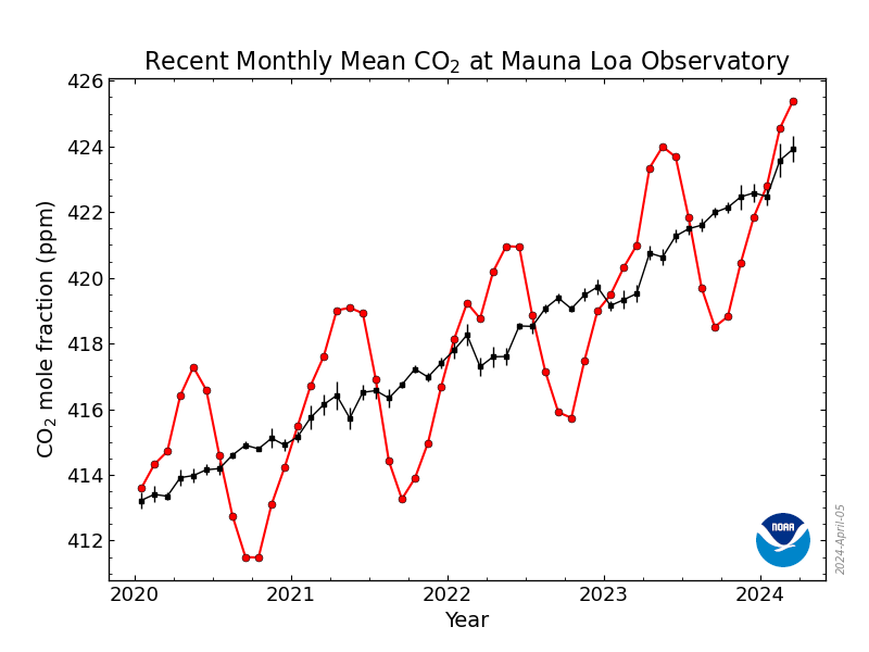
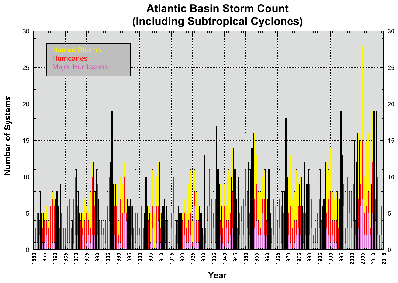
Soil Maps

Surveys of soils are frequently carried out by governments to better understand the availability of lands to different types of crops. The type of soil often is an important determining factor in what will grow in the soil. In the United States geologists survey lands as part of the Soil Conservation Service, currently named the Natural Resources Conservation Service to map out the various soil types in a region of interests. Soils change with land use, climate conditions and the amount of disturbance on the land. Soils increase their organic content over time, but much of this organic content (O and A horizons) is lost due to continuous farming, soil erosion and changes in climate. The increase use of fertilizers is a consequence of the loss of these soil nutrients, which add nitrogen, phosphate and potassium (potash) to the soil. These are required for plants to grow, which normally gain them through the organic decaying matter of dark organic rich soils. When these materials are absence or eroded, then artificial nitrogen, phosphate and potassium (potash) is added to the soil to increase crop yields. This results in high levels of chemicals of nitrogen, phosphate and potassium, with low organic matter entering the soil, with each crop harvest. Overtime the soils become nutrient poor as little organic matter is inputted into the soils, which are turned over with each plowing of the field. Mapping soils become a major way to track changes in the soil profiles over time, and to access the health of the landscape toward agricultural practices.
Palmer Soil Moisture Index

Palmer drought index was developed in by Wayne Palmer in the 1960s to access the changing soil moisture levels using weather data to predict the amount of soil moisture in a region in a given month or week. Soil moisture is of vital importance to overall health of crops and for industrial agriculture. These indexes are able to recognize regions with abnormal drought-like conditions, and access the severity of those droughts. Palmer index maps of soil moisture factor in the duration of the dry conditions and the amount of moisture that is retained in the soil for plants to use. As a short term assessment they can be used to determine when and where droughts occur, and the severity of the drought compared to previous years.
Soil Erosion

Most arable land on the surface of the Earth is disturbed by the rotation of crops, from planting to harvesting, tilling to seeding. Each year a farm is utilized this way, there is a risk of soil erosion, a result of exposed dirt and soil transported due to exposure to rain and wind. This erosion of the soil is particularly dangerous to the agricultural industry, because it rids the soil of the light organic rich matter that provides nutrients to plants and crops grown on the land. Alternating or laying a field fallow, as well as crop rotation can help maintain the soil, and re-generate new organic matter, but often this costs money in having a field not produce crops during a growing season. These trade-offs between planting or not planting can result in more barren crop lands, or longer termed returns on crops. Understanding the over-all health of the land and its soils is particularly challenging given the economic incentives to plant and harvest each year. With the risk of droughts and other weather changes, these farming can be a risky venture, even in the best of times. Protection of soil erosion is enormously important to maintain the yields of crops available for the long term, and help keep food prices from rising. Soils are a renewable resource, but it takes time for soils to reach organic levels necessary to produce high yields, often this is circumvented with the use of fertilizers. With the lack of organic matter, the soils are more prone to drought, due to increased evaporation, as well as erosion from wind and water.
| Previous | Current | Next |
|---|---|---|
7i. Earth’s Ecology: Food Webs and Populations.
Species Habitat and Niche

Across the barren ice tundra of the island of Spitzbergen in the Svalbard Archipelago, a lone fur clad figure hiked across the landscape. Located north in the Arctic circle, the Svalbard Archipelago is a cold foreboding place, inhabited by a scraggily few coal miners who make a scant living pulling out coal from ice covered mines to be shipped south. The islands are technically governed by Norway, but its loose inhabitants come from America, Russia and Germany to work the coal seams, with a tiny tourism industry. However, the islands are nearly unpopulated with so few human inhabitants making the islands ideal to study natural ecology, arctic soils and the biotic world in a place so remote that it has been left to its original natural state, with little human disturbance. This remoteness was what drove Julian Huxley, a professor of zoology at Oxford University to come to the island as part of his travels of the world. Julian Huxley was the grandson of the famed defender of evolution and prominent zoologist, Thomas Huxley. Following in his grandfather’s footsteps, Julian had studied zoology and traveled to Texas to start up a university program in the United States, but with the outbreak of World War I, he found himself enlisted and back in Europe during the war. The aftermath of World War I found him back in his native England, where he took the place of his mentor at Oxford, Geoffrey Smith, who had died during the battle the Somme in 1916. One of Julian Huxley’s pupils at oxford was Charles Elton, and he invited him to travel to remote island of Spitzbergen to study what he could of the native life.
Charles Elton was enthusiastic for the expedition, but many viewed the trip as foolish, since the remote arctic island was noted for being nearly barren of life, with only a few insects and plants, and few if any vertebrates. Nevertheless, Charles Elton accompanied Julian Huxley and started his career in understanding the ecology of life. Elton was influenced by the question of how animals make a living within a community of organisms. The islands have few terrestrial mammal species, including the Svalbard reindeer, Arctic fox, and sibling vole, and wandering polar bears that crossed over the ice feeding on aquatic seals. Attempts had been made to introduce other species, like musk oxen, but they did not survive the cold harsh winters.
Ecologists define two characteristics of every biological species. The first is the habitat of the species, which is the physical geography of where the organism lives, and second is the niche of the species, the way in which the species is able to survive and acquire food and nutrients to live on. An easy way to remember the difference is that the habitat of a species is equivalent to its home, while the niche is equivalent to its job. For example, the Arctic fox that lives on the Svalbard Archipelago, has a habitat across the Arctic tundra, but a niche as a predator of small voles and birds that live on the island.

During his study of the life on the Svalbard Archipelago, Elton was particularly interested in the cycle of population growth and decline in voles, which appeared to rise and fall with food availability. He also noticed that populations of arctic fox appeared to follow the rise and fall in vole populations, since they were dependent on healthy populations of voles to survive. The expedition was funded by the Hudson Bay company, a company interested in fur trapping and understanding the population dynamics of fur bearing mammals. Following the expeditions and his studies, Elton was hired as a consultant for the company to look at the dynamics of population growth and decline in fur bearing mammals in Canada. This allowed Elton access to an enormous amount of historical data regarding the record of trappings of mammals by the Hudson Bay company going back decades. Analyzing the company’s archives, Elton discovered a ten-year cycle in the abundance of Canadian lynx and snowshoe hares. Snowshoe hare populations would rise, resulting in an increase in available food for Canadian lynx, leading to their increase in population, as predation increased resulting in snowshoe hare populations to decline, as the snowshoe hare populations declined the population of Canadian lynx would subsequently decline too, and predation would decrease, this would result in a slow increase in snowshoe hare populations. This oscillatory cycle of population dynamics between the two species was strong evidence for the interconnection of prey and predator populations through the availability of food. The story of Canadian lynx and snowshoe hares is more complex, as the two species are also influenced by the availability of other sources of food, but they illustrated to Charles Elton the importance of food chains or cycles, and the interdependence of species on each other.
Food Webs, Trophic Pyramids and Ecological Communities

A food cycle or food web is the interconnection of food sources into a graphical representation depicting a web illustrating which species are being consumed by other species in an ecological community. Another name for food web is consumer-resource system. You can broadly divide all life into either autotrophs or heterotrophs. Autotrophs are organisms that derive their energy and nutrients from the abiotic environment, for example many plants unitize the sun (photosynthesis), requiring only water, carbon dioxide and soil nutrients to grow. Heterotrophs are organisms that must derive their energy and nutrients from other organisms, for example deer that eat shrubs and grass. These divisions are also called a trophic level.

A trophic level is the number of steps along the food chain (or web) a species is from a primary producing autotroph. For example, snowshoe hares feed on grass and shrubs, and has a trophic level of 2, while the grass and shrubs are autotrophic, with a trophic level of 1. Canadian lynx that feed on the snowshoe hares have a higher trophic level of 3, since they feed on tropic level 2 animals. Trophic levels higher than 4 are rare, as the amount of energy and nutrients decreases with each level, making higher trophic levels susceptible to breaks in the food chain when a prey species drops in population size or disappears. One important addition to a trophic level scheme are organism that feed on dead organic matter, the decomposers, which occupy a unique strategy for food by living on waste or dead organic matter, and depend on this supply of organic matter to feed on for their population growth and decline.

Trophic levels can be depicted graphically into a trophic pyramid, which shows the decrease in total biomass with each level, as availability of food resources decreases with higher trophic levels that can support fewer individuals and less total biomass. For example, the total individual grass plants are far larger than the total number of individual deer feeding on the grass. And the total individual deer population is far larger than the total number of individual wolves feeding on the deer. The total number of individuals of each species is depend on the metabolism and physiology of each species, and how effective they are in the amount of food they required to live.
The idea of food webs, and the interconnection of species is a major concept in ecological idea of a biological community. A community is a group of organisms that live together in the same geographical location and depend on each other for survival. The concept of an ecosystem, induces the abiotic environmental into the concept of a biological community as well, including such influence as climate, weather, water and nutrient resources, availability of light, water depth, water salinity, terrain and geology. All of these factors influence the plants and animals within a biological community.
Ecological cascade effect

An ecological cascade effect is a series of cataclysmic extinction events that occur when a single species is removed from a community, or when an invasive species is introduced that significantly disrupts the community structure. For example, a study led by Ransom Myers and Julia Baum in 2007 found that when sharks are heavily fished and killed in the open ocean, a removal of the top predators (a keystone species) in a marine community, prey species of those sharks (such as the cownose ray) increase in population size. This increase puts additional pressure on bay scallops which cownose rays feed on. This results in a decrease of bay scallop populations due to the increase in predation, and this will ultimately mean that cownose ray populations will eventually decline as well once bay scallop populations are reduced and the number of cownose ray falls without this availability of its food source. This is an example of a cascade effect that quickly collapses a biological community.

Another example of an ecological cascade is a study done by Mark Albins and Mark Hixon (2011) on the introduction of the invasive lionfish to the Caribbean ocean. Lionfish are predatory fish with venomous spines that were introduced to the Caribbean waters sometime in the 1980s. They have few if any predators because of the venomous spines which protect them from larger fish. Since 2005 they have increased dramatically in population size and geographic range in the Caribbean beyond their normal population density in their native habitat in the South Pacific. This is due to the abundant availability of fish in the Caribbean ocean and absence of predators. Lionfish are known to eat large quantities of groupers, snappers and goatfishes as well as gobies, wrasses and basslets, which are important fish for the region. These fish population sizes are in steep decline because of the introduction of lionfish. As lionfish switch to other prey items, such as the parrotfish, the ecological cascade effect becomes more dire. Parrotfish feed on seaweed and algae that grow on coral reefs. By keeping the seaweed from overgrowing the surface of the coral reefs in Caribbean, any drop-in the populations of parrotfish will result in seaweed overgrowing coral reefs, causing them to die because of lack of sunlight. If parrotfish are over preyed upon by lionfish, the overgrowth of seaweed and algae on corals will result in a major extinction within coral reef communities, altering the Caribbean reefs ecosystem. Ultimately the lionfish will become so populated that they will deplete the native fish populations and subsequently fall in population size themselves because of the lack of food— leaving an ocean devoid of many of the previous native species. To combat the invasion of lionfish, active fishing and harvesting of these fish is encouraged.
Population Ecology

When Charles Elton returned to England, he became in charge of one of the most interesting studies of rodent population experiments, when his team turned their interest to vole (Microtus) populations. This was part of the Bureau of Animal Population at Oxford University, a group of scientists interested in understanding population dynamics of animals. In the 1920s it was noticed that large populations of voles were observed in western Scotland near the towns of Dunoon and Strachur feasting on newly planted trees, an area that was part of a reforestation project. These voles increased in population, and then suddenly without explanation would die out. There was little in the way of predators, as many of the foxes and carnivores had been removed from the region, although owls and other birds of prey frequently feed on the voles, there was little sign of increased predation. This cycle of increasing populations and then a sudden crash was puzzling to the scientists, since the availability of food seemed unchanged during these cycles. There was mystery, and many on the team suspected that there was something mysterious about the decline in populations that might be related spreading disease. In 1934, G. M. Findlay and A.D. Middleton published the results of their study.
Voles were captured in live traps to determine population size of the voles in the study area, and recorded over several years. Some of these individual voles captured in the live traps were sent back to the lab to be kept in captivity, and observed. When the population suddenly started its declined, many of the traps became empty, as the population fell. The few voles captured during the population decline period were taken into captivity, but subsequently died even captivity only after a few short days later. Study of the dead bodies of the voles showed signs of lesions and cysts in the brains, related to a parasite called Toxoplasma. Toxoplasma is a single celled eukaryote with a complex life cycle that infects mammalian tissues. Once in a host, the parasite proliferates in the tissue as tachyzoites and eventually forms cysts, called bradyzoites. These cysts proliferate mostly in the brains of mammals, and can alter the behavior of the animal and can cause death. A sick or dying mammal is susceptible to predation, and the parasite can be transferred to a predator, most often domestic cats. Once in the digestive track of a cat, the parasite changes into sexually reproducing merozoites in the digestive track, that can result in abundant oocysts (eggs). These oocysts are shed from the digestive track into the soil, when the cats defecate. These oocysts, which can survive in the outside environment, if ingested can hatch and infect a new host.

Food webs are more complex with the introduction of parasites, such as Toxoplasma. As vole populations increase, there was likely increased predation by house cats, resulting in the surrounding soil to become enriched in Toxoplasma. The increase in the parasites in the soil, likely meant that more voles were infected by the parasite, which made them more susceptible to illness, death, and predation. At peak population, voles were impacted by two forces, the increase in cat population and predation, but also the increase in parasites due to the increase of cats shedding oocysts into the soil. This unbalance, results in a very sudden drop in vole populations. Parasites, and other disease-causing microorganisms should not be excluded from food webs, as they can contribute to dramatic changes in population sizes, that often remain hidden to researchers.
Overpopulation
We can think of overpopulation as the moment in time when the available resources are inadequate for the population to continue to grow. Post peak population decline can be sudden, as in a crash, or it can be protracted, such as a stable plateau or slow decrease over several generations. The rate of fall depends on the patchiness of the resources, and the exponential rate of the decline in the necessary resources for the organisms to survive on. In most stable long-term ecosystems, overpopulation episodes are rare, given the natural inclination for a dynamic equilibrium to be achieved due to the negative feedbacks that stabilize populations of a biological organism overtime. Ecosystems can become susceptible to overpopulation episodes when they are disturbed from their stable conditions, like the introduction of invasive species, or alteration of land use, as well as changes to the physical environment, such as climate changes. These episodes can result in significantly altered environments that can collapse an ecosystem into fewer trophic levels, decrease species richness and biodiversity. Recovery of such events are prolonged, often requiring thousands to millions of years of slow recovery to begin to see increased biological diversity and speciation in those environments. The heterogeneity of the environment also helps partition populations, increasing the likelihood of geographic speciation events in the long-term recovery process.
Overcrowding and Self Organizing Behaviors.

One of the interesting questions explored by science, is whether there is a limit to the density of a growing population. If an organism is given access to unlimited food and resources at what point do they decline. Geographic space itself can be thought of as a hidden natural resource in overcrowded populations, which can lead to population crashes as easy as loss of food availability or other natural resources. Most species have optimum space requirements, which may become limited during overpopulation events. In the 1960s, John B. Calhoun conducted a series of experiments starting with domesticated Norway rat populations, but following with experiments on domesticated mice populations that were allowed to grow in an enclosed limited space, in the absence of predation and any food and water scarcity the population grew. The population grew quickly for the first several generations, then begin to plateau rising more slowly toward a peak of 2,200 within an 9-foot square enclosure, with a density of 20 mice per square inch of floor space, although the enclosure contained tunnels and other partitions. After this peak density, the population suffered a rapid decline, with low reproduction, fighting between individuals, cannibalism and other maladapted behaviors. The surviving population was unable to recover, leading to a complete collapse of the colony of mice. The experiments demonstrated that geographic space is an important natural resource for species, and the limitations of geographic space can result in population decline, equally or more severely as that of food and other resources. In a natural population, organisms will maximize the availability of space to their preferred life style, and self-organize within local groups or isolated units depending on the nature of the niche and habitat requirements, as well as the inner species behavior of the organism.
| Previous | Current | Next |
|---|---|---|
Section 8: EARTH’S HUMANS AND FUTURE
8a. Otzi’s World or What Sustainably Looks Like.
Death on the Mountain

A cold wind blew across the high mountain of Gamskarkogel in the high Austria Alps. For Helmut Simon, the wind was a jarring cold wind for October and the coming winter, as he hiked along the high alpine path in the fall of 2004— his footing stumbling along the path at his advancing age. The thin cold alpine air ran through and tossed his gray beard, invigorated his steps, as his hiking boots with new soles and his wind breaker coat with its thick layers protected him from the elements; he pressed onward up the steep mountain slope. Helmut Simon loved to take different routes on his accent up the mountain, never happy with the well-worn foot path crawled by so many tourists and weekend hikers. A casual hiker was not Helmut Simon, instead he was a stubborn climber, a mountaineer. He navigated up the jagged rocks between the steep towering pinnacles, across paths rarely traversed, but offering an incredible intoxicating view of the mountain tops, and tiny valleys and glaciers that wove down below through the deep ravines. He was an experienced climber, having ascended the mountain numerous times before, up to its cross-bearing top. Little mattered that day, because the strong wind pushed him beyond his capacity to balance himself and he slipped off the rock, losing his footing, and finding himself plunging 300 feet to his death.

Helmut Simon’s body lay at the base of the steep ravine, snow- and ice-covered contents of his possessions entombing him. A backpack, made with nylon fabric sourced from petrochemicals, equip with a metal zipper, forged from iron ore mined thousands of miles away on the other side of the Earth in Michigan, and painted with dyes bound by latex rubber from plants grown in the Amazon rainforest. Inside the pack, was a water bottle, sealed with neoprene, made by the polymerization of hydrocarbons from oil buried deep below the North Sea. A hand full of copper and zinc coins sourced from mined ores found in gigantic holes dug in America and Africa with monstrous machines. His clothes, not sewn by his own hands, but weaved from cotton grown in the hot crop fields in Mississippi, and transported to Vietnam to be spun into thread, and dyed with pigments from Pakistan to be then tread together into gigantic fabric sheets, sewn on machines and with armies of workers he had never meet. His shoes, were leather, from cattle that had lived in South America, harvested and processed in a large meat-packing plant in Buenos Aires, the leather sent to China, and cut into patterns and glued onto latex rubber and petrochemicals sourced from West Texas. His socks, worn and holey from his frequent hiking, made from cotton grown in India, a place he never visited. His backpack contained more complex items, like a cell phone, filled with microscopic parts, sourced from nearly every country in the world, assembled in a giant factory in China and transported to Austria. Its gleaming reflective black screen made of silica, sand melted to its purist form, with zinc mined from the Congo, and gold from the Canadian Rockies, and other conductive metals intricately woven together with an internal processor, that he had never really known how it worked and why. Even the food he carried with him was sourced from widely spaced places on Earth. A food bar, formed by oats and wheat grown in Russia, and grounded down in gigantic factories, and glued together from Iowa corn, processed into corn syrup, and sugar from Cuban. The wrapper, covered in aluminum, a metal that would be so rare and valuable, but people had discovered a process to make it into thin sheets from bauxite ore from Australia. It had become disposable, to be tossed aside after eating the food held inside, to just serve the temporary duty of keeping the food bar fresh. A metal flash light, containing an alkaloid battery, made in Japan, from chemicals and parts from the United States and Mexico, including potassium hydroxide mined from Utah. Nothing Helmut Simon carried with him could be found in the local environment that he lived within, near the mountain top he had died on. No item was made by himself, it was all purchased and traded for. Everything was globally sourced from every continent on the Earth, and even from beneath the ocean. Items made by thousands of workers all located across the Earth coming together to make the wondrous items Helmut Simon carried with him the day he died.
The Iceman


If Helmut Simon was alive, he would know the irony of his demise. Death while hiking in the Austrian mountains was familiar to him. In 1991, while hiking in the Ötztal Alps with his wife, they stumbled upon an ancient frozen body in the ice, exposed from the melting glacier that once encased the corpse. It was mummified, the red body poking out of the ice, with preserved tattooed skin, still associated with his clothes and belongings of this ancient hiker and fellow mountaineer. Radiocarbon dating revealed that the body was over 5,000 years old. A geologic instant in time, still within the modern Holocene Epoch, the age of modern humans, but from a simpler time in the past. The contents of what this Iceman carried within him, contrasts with that which Helmut Simon carried with him on the day he died. The ancient man’s belongings were scattered around the half-frozen body in disarray. They included a long bow and arrows with a quiver. The bow made of yew, a conifer tree native to the region known for its flexible, but strong wood. The ancient man had been working on the bow himself, carving it down with the tools he carried with him. The quiver was made of deer hide that he himself had killed on a hunt. Its leather tong sewn into a tight seem. The arrow shafts made from the branches of the wayfaring tree and cornelian cherry, native in valley floor below. Flint arrowheads were fixed to two of the shafts, banded in plant fibers, and held with birch tar sap from birch trees that lived near his home. The feathered fletching, glued with birch tar as well, kept his arrows straight. He carried a flint dagger, the handle made of ash wood, with a flint blade that was picked up 90 miles away, shaped by a stripped branch of a lime tree grown in the southern lowlands less than 100 miles south, and traded with for some skins. Deer antlers were carved down, to shape and sharpen his flint blade. His most prized item was his two birch bark containers, which held maple leaves and burning embers of charcoal that could be used to light a fire in the night. His backpack was made of two wooden sticks, and two broad wooden planks, that supported a deer hide sewn together to carry his belongings. Among his smaller items was a dolomite stone with a drilled hole, and woven leather strips used to carry caught birds, and birch mushrooms, used to treat scratches and injuries as a first aid kit. The most valued and complex item was his copper bladed axe, which was formed from copper ore (native copper) mined in South Tuscany, about 275 miles away. By far the farthest sourced item in all his possession. Everything he died with was local.
Only 5,000 years divide Helmut Simon and the Iceman (famously named Ötzi), yet the items they carried with them on the day they died reveals the major shift in human consumption of the modern age. Indeed, all humans, even the ancient Iceman Ötzi used natural resources from the Earth, and were dependent upon them for their survival. But the items carried with Helmut Simon were sourced from a broad global network, that involved thousands of people that the Iceman could only dream about. In contrast, the Iceman’s ancient items are all locally made from the plants, animals and rocks that could be found nearby or traded with. In our modern eyes, the ancient Iceman was living a sustainable life, with little if any impact on the Earth. The Iceman was not simple person, but showed great knowledge in understanding the world around him and the ability of surviving using those limited local items.
Sustainability
Sustainability is the ability of a society to maintain its current rate and level of growth. Sustainability in the age of the Iceman was likely based on the availability of food and the danger of overhunting and competition with other tribes and groups. In fact, from what we know of the Iceman’s death, he was murdered, shot with an arrow during a battle on the high mountain, over what grievous we don’t know. The life and death of the Iceman was harsh and cruel. He suffered from parasites and illness, with a much shorter life expectancy than modern humans living today. We may find his lifestyle of zero waste and living off the land, something to emulate in the modern age, but given the much larger population of individual humans living today, the required space, forests, plants and animals necessary for this primitive lifestyle exists no more, having been stripped for timber, mined and developed with road and asphalt streets and fenced under private ownership.


The story of the Earth’s transformation under an ever-growing population of humans is one that has played out in tragedy after tragedy in the short period of the last several centuries. The Earth stripped of its natural resources has become a landscape that forces humans to adapt to ever unsustainable practices. Open pit mining, oil and gas development, timber and forestry, industrial scale agriculture and the urban growth of cities have all lead to an Earth that is very different from the age of the Iceman 5,000 years ago. The modern age of humans on the Earth of today was created from the extraction of its resources for the establishment of a single species, a species that has grow to dominance on the planet, unparalleled throughout Earth’s long history.
Earth has conclusively transformed with the widespread presence of humans on its surface. There is little that separates the natural wild lands of the ancient past, and the urban industrial centers of the modern age. Earth can no longer be said to be divided into nature and non-nature, of cities and wilderness, for wilderness has become so altered and changed, disturbed by the meteoric rise of populations and the demand for resources from the Earth, and the churning waste and pollution that has metamorphosed Earth today. Ultimately the rise of humans cannot be uncoupled from the complex interaction of the Earth’s atmosphere, solid interior, oceans and water, and the multitude of other organisms that humans share the Earth with. You are destined for an Earth that is filled with impulsive fears, anxiety and insecurities that are reflect in our own depression and deprivations in the modern age, and guilt over this transformation of the Earth.
It is important to remember several factors in this transformation of the Earth by the hands of humans. First, humans are made of the Earth itself, and have evolved through the natural processes that have operated on Earth’s surface for its billions of years. You and your ancestors, and those before them, have been part of the cycle of life on Earth. Earth is our home and place in the universe. A candy wrapper in a field, is equivalent to a fallen leaf from a tree, both refuse from Earthlings, of living organisms composed of material found on Earth, and changing and altering to its current state. Earth differs from most other planets in its ever-dynamic change and transfiguration, part of this is brought about by its life forms. The rise of an oxygen rich atmosphere, transformed the way life evolved, just as the rise of a carbon rich atmosphere will further transform life into the future. Plants will flourish longer, climates will warm, even if humans die with choking breath, and mass graves are dug.
Second, Earth has no obligations to maintain its environment or habitability for humans to exist within. The Gaia and Medea theories of a balanced environment at equilibrium, or a chaotic cataclysm of death and the apocalypse, are views along a continuum. The Earth can be balanced, or knock on to its side, or somewhere between. There are unintended consequences for our actions, often actions that received little thought or foresight to those that are appointed to make these decisions.
The third important factor in the transformation of Earth’s surface by humans is that we face this change with unhappiness. It is, after all, difficult not to feel restless, hesitant, and unhappy when imagining Earth changing from the world before human alternation, into what it is today. However, this unhappiness is a result of a pervasive lack of imagination for Earth’s future. Much of this unhappiness can be set aside if we can overcome and solve the pressing issues facing the Earth, its habitability, and making it a better place to live within for ourselves and the many diverse life forms that live on our planet.
This next section of the textbook will examine humanity and its complex interactions with the Earth through its consumption of natural resources.
| Previous | Current | Next |
|---|---|---|
8b. Rise of Human Consumerism and Population Growth.
Ecological Economics

The United States has frequently been caricaturized as a citizenship of excess consumerism. Homes are disproportionately large for the typical family, with multi-car garages, manicured lawns and laid out in widely spaced suburban patterned streets. Houses are cooled during the hot summer with automatic electric air condition and heated in the winter with gas furnaces. Paved roads interconnect towns and cities, with wide interstates filled with large vehicles and trucks. Over these wide roads which cover vast regions, they provide daily commutes using large cars and trucks fueled by gasoline and diesel. A network of pavement between shopping centers, markets and places of employment at factories or offices, and the various leisure activities, making up these urban centers. Parking lots have replaced meadows and forests. While farms are now industrial scale, using large machines to harvest and plow large tracks of land. The wildlands cleared for timber, stripped mined or developed into industrial oil and gas fields is the predominate landscape of rural regions of the country.
Living within the urbanized Earth, it is difficult to fathom how we reached this pinnacle and precarious perch that humanity now stands upon. Humans have transformed the Earth in the last 200 years, changing its atmosphere and altering its oceans, with a swift progress that involved unique ways of cooperation. Study of this complex human cooperation through production, distribution, trade, and the consumption of goods and services extracted from the Earth is known as economics. Ecological economics is the subfield interested in how humans interact with the Earth, and emphasizes the need for sustainable practices that protect life on the planet from collapse.
American Mineral Baby

The Mineral Education Coalition publishes an estimate of the amount of raw minerals and rocks the average child born each year will use throughout their life. In 2019 it is estimated that every American will have used in their lifetime, 15 tons of salt, 7 tons of phosphate limestone, 6 tons of clay minerals, 26.5 tons of cement and lime, 10 tons of iron ore, 1 ton of bauxite for aluminum, 680 tons of aggregate for roads, construction and pavement, 165 tons of coal, 980 pounds of copper ore, 953 pounds of lead, 466 pounds of zinc, 31 tons of other metals and minerals, like tin, lithium oxide, and rare earth metals, with 75,327 gallons of petroleum and 7.7 million cubic feet of natural gas, and 1.5 ounces of gold. This does not include the amount of food and freshwater that a person needs through their whole lifespan. The total land required to meet these demands and are used per individual, is known as the ecological footprint—the land required to sustain the use of these natural resources from the Earth. The concept of an ecological footprint was first developed by the work of the Swiss scientist Mathis Wackernagel in the 1990s as a method to estimate the amount of space required per individual to live on Earth at their current consumption habits. This was expanded into the Global Footprint Network, which offers a Footprint Calculator for you to estimate the amount of space required, as well as the amount of Earth’s total surface actually required if everyone on the Earth lives as you do. The results are frankly startling, as the capacity of Earth is nearing its limit for the number of humans that can occupy the planet. This point in time is known as an overshoot, which occurs when the resource consumption exceeds the availability of those resources to maintain the current population and living standards. Overshoot events are thought to precede a sudden collapse within a society, as the resources are no longer able to match the necessary demand, which leads to scarcity, starvation, and general population drop depending on the resource in decline.
The Rise of Human Consumption
The modern human species Homo sapien arose on Earth between 300,000 to 200,000 years ago, and for most of that time, humans utilized only the local resources of their immediate environment, such as plants, animals and water as well as natural shelters such as caves and other constructed homes from natural materials available. The rise of human consumption during the recent period of human history has been very rapid with the advent of human civilization. Civilization started with technological advancements in the domestication of animals (starting about 20,000 years ago) and the advent of agriculture (starting about 11,000 years ago). Since then, humans have become more cooperative with a complex network in the trade and exchanging of goods and items. This profound shift in using the Earth’s resources for the production of goods that are to be traded, lead to the rapid changes that you observe today on the planet. The growth of trade allowed for the extraction of natural resources to produce and distribute goods to widely spaced geographic areas around the world. This was accomplished in three stages that lead to the modern rate of trade and commerce that we have today.
The Origin of Taxation

Increases in domestication and agriculture came with the issue of protecting those place-bound resources from other groups of humans, which would attack, steal, or destroy those resources, and blunder those goods. The more production increased, the greater the need for cooperation between and among humans to guard and protect those resources. They also needed to be able to trade goods with other groups lacking them in exchange of goods scarce to their own region. These early trade routes and guarding armies required a percentage of the profit to flow to people not directly involved in the making of the goods themselves, this resulted in groups of traders and sellers exchanging goods, as well as taxes being levied against these trades. These profits resulted in a percentage of the exchange to flow through a community of people, eventually leading to an important aspect of civilization— egalitarianism. Egalitarianism is the idea or philosophy that all humans are equal and should be treated equally in a society with the sharing of profits and goods.

However, these early communities were far from being truly egalitarian, as they were besieged by tribalism and nationalism. Brutal wars, murder, genocide, and systematic violence was feverishly common between groups and individuals. These breakdowns in early civilized societies would result in their frequent downfall. Traders were often put at great risk in moving goods across the Earth without protection. Slavery existed, where an elite group regarded fellow humans as goods themselves, to be traded and forced to work, resulted in inequalities in these early societies. These inequalities persist into the modern age. Taxation likely developed from extortion and bribery, in which groups rather than bunder all the traded goods, would take some part of it, knowing that by killing or robbing the traders, they would lose the long-term access to these goods themselves. Taxation was a method of dividing profits to serve larger groups of individuals.
The Origin of Bonds

Taxation comes with the issue of having wealthy groups that might rebel when forced to pay these costs, and since they are wealthy they could hire their own army and overthrow the local group of elites if the taxes became too high. The development of contracts, or agreements between a ruling class and noble class in a society, lead to the early ideas of feudalism and land ownership. The most famous of these changes can be found in the Doomsday Book, or in Latin the original title Liber de Wintonia. In 1085, William the Conqueror ordered a survey of the land and goods that they had conqueror during the Norman conquest of England and Wales. These early surveys were meant to establish rights to individuals to own land, and establish taxes and fees to those entities. It was called the Doomsday Book, because people living on the land or in the region not recorded during the initial survey were subjected to servitude and lacked legal authority to the land. These surveys resulted in major inequalities between the upper-class landowners and those lower-class peasant and serfs that were required to work the land, but not own it. Such concepts of landownership resulted in increased need to produce crops and livestock to trade or sell in markets, and trade for goods that the particular parcel of land was unable to provide for. During this time, cities grew as places of trade and commerce, since each parcel of land resulted in different goods and items that required exchange at the markets and in the city centers. This process of dividing the land into parcels with a legal authority governing who owned what resulted in a major transformation of the Earth’s surface. It also promoted slavery and servitude to work the land, with the benefit of a wealthy landowning upper class. These primitive societies were still susceptible to invasion, attack and revolt. Often small city states hired mercenary forces to protect these lands, as well as standing armies who were overseen by nobility, such as a king or queen. Much of these services were paid for by taxes, which helped maintain the legal authority of landownership, by contributing to these standing armies or mercenary forces. However, many nobles receiving these taxes realized that the conquest of new lands could be of major benefit to them, as they would expand the revenue incoming to their own courts. However, if these armies pursued a war and lost, it would offer a major risk to the current landowners on the losing side. Landowners were not supportive of these efforts to invade other countries, until the advent of bonds. The concept of bonds developed around 1590 as a way to bind individual nobles together by offering loans to the rulers, which would be paid back with interest by the rulers or government. These came about with the increased cost of conducting wars and conquering other nations, such as the advent of firearms and other specialized weapons that required more money. Bonds unified the upper class, allowing the distribution of wealth to remain among the elite landowners, who benefited from exploits of wars and bounty during various conquests of exotic lands outside the boundary of their own nations. This was the age of colonization, which would see great global empires arise for the first time on Earth during the 1600 and 1700 centuries.
The Origin of Stocks
.jpg)

Local trade between one region and another became less risky the stronger the nation’s governance. However, shipping goods across an ocean to a far-off colony, carried much more risk if the ship sank or was attacked by pirates, and greater returns, in that what goods the ship traded for and carried back would be exotic and worth considerably more that the goods shipped out. To mediate this risk, stock was offered in which a ship owner would receive money before the goods were delivered, and then payout money with profit on the return of the ship, such that if a ship were to sink on its long journey, the ship owner would not have lost all the value of the goods and the ship. These types of transactions lead to a greater interest in making these risky trading trips around the world, and the exchange of goods across vast oceans between conquered lands. The concept of stocks would revolutionize the export and import of goods, and the increase demand for natural resources across global trading routes.

Raising Capital

The rise of global trading routes financed by investors who would buy stocks in the ships at ports allowed a network of trade that made international trade possible, and resulted in a possible path for individuals to gain money and status in a society to own land, while not being of the noble class. People were attracted to investing with companies of individuals engaged in the trading and exchanging of goods. The windfall that befell those investors, resulted in a path toward landownership and becoming viewed as an elite within a society. This possibility of individual prosperity also calmed turmoil among the people locked within servitude. However, this pathway was limited to a select few, but during the age of enlightenment and the stages toward emancipation and freedom of slaves, this possibly of investment in stocks and bonds opened the door to a greater number of individuals with means to actually make those investments. This system of government is called capitalism. Capital is the equipment and materials required in the production of goods. For example, a ship and its crew would be regarded as capital in an expedition to trade within an exotic port, but so would the goods to be traded be regarded as capital. Sometimes these are referred to as capital assets.

The United States of America benefited greatly with this style of capitalistic society, as it was founded on the eastern seaboard of the North American continent, with trading ports between its shores and those of Europe, the Caribbean, and even North Africa. It also had a source in the interior lands of a continued conquerable lands from the native indigenous peoples of the interior. Between 1800 and 1850, in fifty short years, the United States purchased and conquered much of the western region of North America. As already occupied by native people, and being more arid and difficult to access, it nevertheless rapidly changed the ownership of this land during the years leading up to and after the American Civil War. In an attempt to quell the Civil War in the east, and to restore pathways to landownership in the interior, the government begin the process of giving land away to eastern settlers. This land reallocation pushed people in the east to go west to establish farms and towns in the more arid climates, and lead to conflict with native people in these regions. This great westward migration resulted in major conflict of the people already in the region, and also led to a completely alternated landscape, with the promotion of agriculture and landownership, as well as the major extraction of mineral resources found in the region, including gold and silver.
The Journalist and Mathematician
Charles Dow was born on a farm in Connecticut near the Rhode Island border in 1851. His father died when he was six, and the family struggled during the Civil War. He nevertheless enjoyed reading and writing, and aspired to become a journalist for one of the many newspapers in the region. In 1877, he finally was able to find a job writing for a newspaper, and took an interest in the history of Newport Rhode Island. Newport was an important trading post since its colony days in the 1600s, but faced an economic collapse, but subsequently had become a revitalized port after its initial collapse. The town’s story was tied up with the whaling industry during the mid-1800s, and the massive efforts in harvesting whales for oil used in lamps and cooking, which were exported around the world. During this massive harvesting of whales, the population of along the North Atlantic collapsed, leading to a scarcity of whales, and a collapse of the local economy. To make money, the local population turned toward the illegal slave trade and the manufacturing of rum from imported sugar cane from the Caribbean. The American Civil War and freedom of slaves, ending these trade routes, which left a low value to the lands near the port. Many southern plantation owners moved north, and started trading in ginseng rather than cotton, that could be grown in the local climate and did not require large workforces of slaves that were now freed. Ginseng was exported to China which made fortunes and these people established large plantation style homes in New England, in the style of southern plantations. This transformation of Newport fascinated Charles Dow, and he wrote of the ways in which fortunes were made and lost in the town since its founding.

In the 1870s during the reconstruction of the United States from its Civil War, individual investors were interested in investing in mining stocks. Many companies were looking to raise capital for the extraction of gold and silver from western mountains, which was heavily supported by the government with the passage of the Homestead Act in 1864 and switch to a gold standard for coins. However, unlike a ship and its goods, where the investors could inspect the vessel and items before setting sail, far off mines in the rugged regions of the interior where highly speculative, as most stocks were sold with no intentions of developing the mine, or demonstrating to the investors that the mine would produce gold and silver. This speculation was made all the more problematic because of the Homestead Act, and the giving of land away to white settlers, with the explicit rule that it be developed for agriculture or for mining. It was tempting for an individual living on the east coast to raise money to develop a mine somewhere west. However, if they gave those funds to a company that either disappeared or developed the land with little to no intention to make a profit, they would lose all their money. Fraud was common and many people lost their fortunes on such ventures. The government subsidized this great migration westward with finance speculation because it afforded the eastern states access to the interior of the continent and dispersed the warring population and fractions that had developed after the war. The government helped finance a transcontinental railway, giving large tracks of land to the railroad companies. All this required capital, funded through selling of stock to individual investors. For some, the risk proved very profitable, while others saw their fortunes evaporate. In 1879, Charles Dow was asked to cover a news story about the mines in Colorado, and he traveled to the gold and silver mines of the rich district in the country, the old west mining town of Leadville Colorado. There he quickly understood the pitfalls of east coast investors, as they did not know which mines were profitable ones and which mines were simply plywood cutouts and decoys to garnish more investments. Dow wrote nine letters from Leadville, concluding that mines are extremely risky investments and require insider knowledge of the mine and its true profits before one could invest in these stocks. On his return, Charles Dow realized the need to communicate financial knowledge about companies and their profits as an independent source to the public. The idea was sparked by his continued friendship with his friend at the newspaper Edward Jones. Jones was a mathematician, but also wrote for the paper and they discussed the importance of providing information to investors about the profits of companies and their worthiness in investing. They were joined by Charles Bergstresser, who suggested that they name their newspaper the Wall Street Journal, after the name of the street were the New York Stock Exchange and Treasury Building is located in Manhattan. This newspaper grew in importance because of the list of reputable companies that they published, which became known as the Dow Jones Index. The Dow Jones Industrial Average (DJIA) is the total stock of 30 companies that are ranked by the newspaper, often large capitalized relatively safe companies to invest with. These types of indexes had a profound effect on the flow of money into the most productive companies, which were subsequently able to exploit more natural resources from the Earth, through an increased drive for profits. Where before stock purchases were very risky, now for companies to be listed on the Dow Jones they had to prove to the public that they were productive, and this production self-drove continued investment depending on investor sentiments of growth and production. This made companies overproduce, and often this overproduction was driven by government incentives.

These cooperative agreements meant that citizens, companies and even the government all worked together to incentivize the production of goods without consideration of the environmental damage these endeavors cause. In the case of the gold and silver mines, these were driven by the actual purchases of gold by the government itself. During the Civil War, inflation plagued the dollar, which became uncoupled from the price of gold. In the early 1870s the U.S. Government begin purchasing gold from these western mines to back the dollar and restore the dollar’s value. Price fixing became a major issue, and forced the U.S. Government to suddenly drop their order for gold from the mines in 1873 to bring down the price. This resulted in a rippling effect through the economy and the collapse of the value of the dollar, as people exchanged dollars for gold. However, in the decades to follow, silver coins became worth less than an equal currency value established for gold coins. So, investors bought silver, exchanged it at the mint for gold coins, and then sold these gold coins in the market for more than they had paid for using silver turning a profit. Quickly gold became scarce and much more valuable than silver. Mining companies had extracted large quantities of silver (which is more common than gold), resulting in an oversupply of silver metal. To fix this issue, mining companies lobbied the government to begin buying large amounts of silver and issue fewer silver coins, to keep the mines open and running. This oversupply of silver continued since the government was buying this silver, which resulted in a drop in the price of gold relative to silver. In 1893, people who held gold lobbied the U.S. Government to stop buying silver. They did this, as the government then passed into law that they would no longer buy silver. The price of silver suddenly dropped, resulting in a crash in the price of silver in 1893, resulting in massive economic loss in the western states in the silver mines.
Boom and Bust
The cycle of boom and bust are driving by the supply and demand of goods and the markets that they are purchased within. Trading of goods is driven by perceived scarcity, and the demand of those goods by other individuals, however these perceptions can quickly change in any economy. Many of these boom and bust cycles are driven by governments who push markets in key ways to support stock owning citizens, lobbyists and companies that donate to election campaigns, and receive kick-backs as part of these cooperative agreements. The boom and bust cycle of extraction of resources results in major large-scale depletions of natural resources followed by collapse, and leaves depleted often exhausted supplies of those goods. Many of these goods are not often necessary to living.
Most resources are non-renewable, and scarcity will increase over time, until alternatives are found or demand decreases. With governmental purchases and large scale subsidizes there will be an increase in demand, while governmental regulations can direct companies to find alternatives and prevent scarcity and depletion of natural resources. The middle ground is to have the government do nothing, called Laissez-faire capitalism, discussed by Adam Smith in his classic history of economics The Wealth of Nations, published in 1776, the same year the United States declared its independence. The ideal of laissez-faire capitalism has prevailed in discussions of ways to govern since the inception of the United States. It however has proven to be disastrous in the promotion of the rapid depletion of natural resources.
The consequence of laissez-faire capitalism leads to what is called The Tragedy of the Commons, a concept developed by the ecologist Garrett Hardin in 1968. The Tragedy of the Commons is best illustrated with a simple example. Imagine a tiny nation composed of a single forest of 100 trees, and a population of 4 individual people who make a living cutting trees and selling the lumber. Each tree takes 10 years to grow back. If each individual agrees to cut only 1 tree each year, then the forest will never run out of trees, as the rate of cutting trees is less than the rate of regrowth, and the number of trees will remain around 64, after 10 years. However, imagine that one of the individuals wants to make a little extra money, and cuts 3 trees instead of just 1. In just 32 years, the forest will be depleted and exhausted. With laissez-faire capitalism there would be no penalty for this action. This example using the Tragedy of the Commons highlights the susceptibility for the rapid depletion of shared natural resources when there is little to no regulation and enforcement for the protection and the long-term preservation of the resource. The Tragedy of the Commons also highlights the incentive to cheat within laissez-faire capitalism to turn a greater profit. Simple laissez-faire capitalism always leads to rapid resource depletion when there is strong demand and little protection for a resource. Most countries today don’t apply a purely laissez-faire capitalistic government. Governments can choose to regulate and conserve or protect their natural resources, such as limiting the number of trees cut down per year, to avoid harmful effects.
Using our prior example, imagine that the 4 people of this forest nation is ruled by an elected president. During the campaign to be president, the candidate makes note that their country imports more wood each year than they can sustainably cut down. This is known as a trade deficit. Each year they have to buy 2 trees worth of lumber from another nation. This is expensive and the citizens want more jobs cutting trees. The candidate makes the promise that if elected they would select one of the individuals to get special permission from the government to cut down an extra 2 trees. The 4 people of this nation are excited at this possibility, as they could become much richer if they are selected for this extra source of wood.
Each pays the candidate money to swing favor toward themselves. This makes the candidate wealthy, and able to buy more ads and promote themselves politically. Once they win, as the president of this tiny nation, they award the extra tree cutting to the one individual who gave them the most money in their campaign. That individual is allowed to cut down 3 trees without penalty, increasing their wealth at the expense of other citizens. Since the depletion of the resource takes time, the loss of the forest resources because of this extra cutting of the trees occurs long after the president is no longer in office. Such methods of governance is very common around the world and is referred to as a kleptocracy, a government with corrupt leaders that use their power to exploit the people and natural resources in their own nation in order to extend their own political power and wealth. Such forms of government lead to ecological disasters that result in major poverty for the population with the long-term depletion of natural resources for these short-term gains.
Peak Oil and the Economics of Hydrocarbons
No other product on Earth has driven economies in the roller-coaster of boom and bust cycles than hydrocarbons, like oil and natural gas, which are extracted from the subsurface. Petroleum was discovered in the subsurface in Pennsylvania by Samuel Kier in 1849, and was first used as a medical oil and ointment that he started selling in drug stores. This raw crude oil was discovered when drilling water wells in the region, as it floated above the denser water in the wells. It was soon discovered that this oil could be burned in oil lamps without much odor once it was refined and distilled. The oil through heating would be separated out into the various hydrocarbon compounds, each of which would produce a different fuel source, such as natural gas (methane), propane and octane. Early on, oil wells were drilled across Pennsylvania with the increasing demand for the oil in heating, cooking and gas for lighting, as well as a fuel (gasoline) for early combustion engines. Following the Civil War demand exploded as the number of whales (an early source of oil), became depleted. Production peaked around 1890 in Pennsylvania as drillers drilled deeper into the subsurface to find oil, finding less and less. A typical oil well only lasts a few years, before the oil is depleted and runs dry. Oil takes millions of years to develop in the subsurface, so it is a non-renewable resource, and every well drilled has a typical lifespan of only 3 to 15 years on average, with many dry from the start, but injections of water and gas can to help push oil into a producing well, and extend its production as long as 30 years at limited production levels. The increased demand for oil was rapid with the creation of motorized combustion engines in the twentieth century, and as people purchased cars and trucks, to replace horses, they needed a fuel source for them. Further demand came from the transportation of goods and supplies carried by gasoline powered trucks rather than coal and steam locomotives. This rapid demand for petroleum, resulted in oil drillers moving further and further westward in search of new locations (called plays), with major discoveries in West Texas in the Permian Basin, Southern California near Los Angeles, as well as Wyoming. Many of these sources of oil were owned by landowners who held the mineral rights, but a large majority of these oil fields are owned and managed by the United States Government. The government would lease these lands through the Department of the Interior for companies to extract the oil for profit. In many other countries sources of oil and gas are also extracted directly by government owned companies. This arrangement often led to corruption, for example during the Warren Harding administration in the United States, the head of the Department of the Interior (Albert B. Fall) received personal bribes to issue exclusive access to oil fields in Wyoming to a select number of companies who paid him for those rights. He was later sentenced to prison in 1924 for corruption. Governments encourage the drilling of oil, since it provides a source of income (often as fees and taxes), as well as a cheap energy sources for personal vehicles and trucking transportation, as well as airplanes and air travel.

In the 1950s, cities became interconnected by major Interstates built by the government that decreased travel times between major cities across the country, which was quickly replaced traveling by rail. Such changes in the society demanded more and more oil, with increased demand to travel by these large roads paid for by the government, and this led to a peak in the domestic production of oil in the United States in 1973, after this date oil production begin to drop as the resource became depleted. With production falling, and demand still rising, oil prices soared nearly 400%, and many gas stations ran out of gasoline to sell to its customers. Much of this shock came from the embargo of imported oil from the Middle East, and the fact that domestic oil production could not keep up with increasing domestic demand. The effect of this shock, resulted in high inflation and requiring major downsizing of motorized vehicles. Most importantly it led to increased fuel standards to increase the mileage and amount of fuel needed to travel any distance. From that point onward, the United States carried a trade deficit and had to import much of its oil from other countries, particularly Saudi Arabia. During this time the major oil producing nations formed the Organization of the Petroleum Exporting Countries (OPEC) to set prices on the international exchange of oil, these countries had an excess of oil, and were willing to work cooperatively to set prices. The United States became depend on these sources of oil, leading a continued push (sometimes turning to war) to make these oil markets low in terms of price, but also pushed for innovations to make cars more fuel efficient.

As a nation of widely geographically distributed citizens, the reliance on hydrocarbon sources of fuel continued. Technological advances to extract more oil continued in the 1980s, particularly exploring remote regions like the Northshore of Alaska, as well as deep ocean drilling in the Gulf of Mexico. Technology also lead to the widespread use of directional drilling and horizontal drilling to tap into smaller pockets of oil in abandoned fields. In 2003 drilling expanded into previous regions long abandoned, particularly Pennsylvania, North Dakota, and eastern Utah, with the discovery of fracking, which is the process of introducing acids to dissolve rock in a well, which releases locked oil and gas within pore space inside layers of sedimentary rock. Some fracking technologies used injected gases or explosives and other mechanical ways to break open the rock. This process enabled producers to scrap the bottom of the bowl, and increased domestic production to near its 1973 peak, but this source is limited, and will be soon exhausted. Alternatives need to be found. Oil and gas are both consumables, which means they are used within a relative short span of time, and cannot be recycled or reused.

Consumables include food and oil and gas, while most other natural resources can be recycled and reused once they are extracted like gold and silver, but also glass and many metals like copper and iron, as well as wood and some plastics, although wood and plastic have a more limited recyclability compared to metals. Technological advancements have worked to increase the amount of recycle paper products as well as glass and plastics, but many would be considered consumable (used only once), however hydrocarbons used as a fuel are never reused, and instead are consumed by burning them to produce energy and carbon dioxide, as well as other pollutants. This makes demand much easier to predict since new sources are continually needed. These types of ventures result in ecological impacts to the regions that oil and gas wells are installed upon, covering vast regions of the Earth’s surface. Pipelines and roads are constructed (especially necessary to carry natural gas), and native vegetation and wildlife are disturbed or killed by this industrialization of rural regions of Earth. Oil spills, and deadly explosions at wells and in the petroleum distillation facilities near cities, as well as the pollution caused by the burning of these fuels all contribute to ecological collapse and rapid climate change.
Governments, particularly politicians wield enormous power in the preservation of the Earth through their policies and economic incentives. A large percent of the oil and gas reserves, as well as timber and meat production are carried out on government managed lands, which incentivizes its use and consumption for profit. Such governance can result in long term economic collapse, as the ecological costs of such ventures are often destructive to the long-term health of Earth’s water, atmosphere and lifeforms. Developing nations are particularly susceptible to these investments and projects which are often fraudulent, especially where there is rampant corruption. The United States is not immune to these problems and issues.
Conservation verses Preservation

Conservation is the prevention of the wasteful use of a natural resource, by extending its use over a long interval, while preservation is maintaining a natural resource within its original or existing state. Preservation of land is the action of protecting the landscape by eliminating its use for industry, agriculture and urban development. Preservation retains the landscape and its natural resources to its original form in perpetuity. Conservation on the other hand, allows the use of the landscape, but limits this use to a set quota. Examples of conservation include hunting and fishing limits, limits on tree cutting in National Forests, and fishery limits for wild caught seafood. Conservation requires close documentation of the available resource at any given time, and the amount of use to prevent the depletion of a resource.
Population Growth (r and K)
The human population on planet Earth in 2020 stands close to 7.7 billion individuals, and the population has been rapidly increasing since 1800, when the world population was only around 1 billion people. Population growth of humans has grown exponentially over the last two hundred years. Prior to the advent of world trade and commerce the growth rate was very slow, only about 0.04% annually. After 1800, with the advent of global trading routes and growing commercial exchange of goods between various regions of the Earth, the human population exploded, with a rapid increase to 3% annual growth rates, resulting in 7.7 billion living people living on the Earth today. The Earth has more living human individuals on its surface than any time throughout its long history. It is estimated that about 108 billion human individuals have ever lived, and about 7.3% of those people are living today. There is great concern if the Earth can handle such a dramatic increase of human individuals, and this rapid increase in population density. Resource depletion and the allocation of those resources as they become more scarce fundamentally runs the risk of population collapse in the future.
Ecologists who study population change over time have observed two styles of population growth in nature. The first style of population growth is called r (lower case r), which stands for reproduction. An r or reproduction population growth curve is where a population rapidly increases dramatically, but then crashes very suddenly when it is culled back by increasing death rates. The reproductive strategy of these species of plants and animals is to produce the greatest number of offspring possible. Such organisms, include dandelion flowers, which will produce millions of seeds that are dispersed by wind each summer, with the majority of seeds not growing into new plants. Another example are rats or mice, that often have large litters of offspring, and if there is available resources populations can rise suddenly and dramatically.

This style of reproduction strategy ensures that some individuals will survive, even at the expense of the majority. Species that exhibit these boom and bust population explosions are often very effective of exploiting a resource that is disturbed or undergoing major changes, since they are often the first species to colonize or occupy a disturbed region. The second reproductive strategy is called K (upper case K), the K stands for the carrying capacity, which (actually is spelled with a c). These species produce far fewer offspring, and spend more time and resources for their care. These species will also increase in population over time, but at much slower rates than r strategists. The K strategists will however reach a carrying capacity, that is a population that is balanced between new births and new deaths, such that the population is said to reach the carrying capacity. K strategists tend not to collapse, but will maintain this population for long periods of time. However, this strategy comes at the cost that it requires more offspring care and protection, but also that if disturbed, the population will not replenish itself for a long time.
The question that our current human population poses is whether humans are fundamentally a r strategist or a K strategist? Since humans spend much time in the raising and education of their offspring (especially compared to a dandelion), the clear agreement among most scientists is that humans are K strategist, and that given time the human population will at some point reach a carrying capacity, and remain stable.
What is the human population that the Earth can support?
Some scientists argue that the human population has already overshot its carrying capacity, and that resource depletion as well as atmospheric changes in carbon dioxide and climate change, and limited food production, as well as diseases and pandemics with overcrowding, the human population will dramatically be reduced in the near future. Other scientists argue that the human population will soon reach its carrying capacity of the Earth and stabilize, with some estimate of human population between 8 and 10 billion people as sustainable. These scientists predict that population size will began to slow, as families reduce the number of children, with two or fewer offspring. These scientists are led to this conclusion based on economic data, which demonstrates that the more affluent a family is, the fewer the number of children they will have. More affluent families often are led by mothers who have more rights and say in the raising of their children, as well as their productive role in a society. The more that is invested by a society in raising and educating children and supporting woman’s rights, the slower the population growth of that country, compared to countries that have limited access to education and health care.

Hans Rosling the late medical professor from Stockholm Sweden developed unique ways to visualize human population growth with a key insight into the response of economics and standard of living in relationship to population growth. He and his family, developed innovative tools to observe how countries population dynamics respond to the economic conditions within a country. He, along with his daughter Anna Rosling Rönnlund and son Ola Rosling developed a data viewer called Trendalyzer, which uses data from the World Bank to look at the dynamic nature of population growth and personal income. The results of this massive study suggest that as families become more affluent with increasing income, access to education, and healthcare, they reduce the number of children they have in a family and population growth slows. They conclude that Earth is approaching its total human carry capacity and will stabilize around 10 to 11 billion, as both personal income and life expectancy increases. The opposite is true as well, if families in a country reduce the average number of children in their family through family planning, then over time the average personal income will subsequently increase. This is exemplified in China, which from 1979 to 2015 limited the number of children a family could legally have, resulting in an increasingly affluent country and rising GDP, with a rise in average income for those families as the population of the country stabilized. This idea, that as individuals become more affluent and wealthier, population growth slows and ends, has been refuted by many scientists as being overly optimistic. Part of this comes from the fact that the more affluent and wealthier a person is, the more resources from the Earth they will use. Another observation is that as a human population becomes more affluent and wealthier they exhibit longer individual lifespans, with an increase in life expectancy well unto 80 years of life on average and may give a short-term increase, or bump in population growth instead. The idea that as populations became more affluent and wealthier they reach a carrying capacity and stop growing in population size has been contested in a number of interesting studies (maybe best summarized by Jared Diamond’s book Collapse). It nevertheless is a prediction that in the short-term human populations might began to hit a ceiling.
In the scientific field of economics, many studies have tried to examine the boom and bust cycles of local aspects of economics, suggesting that long term patterns might emerge, where an economy or society goes from a rapid expansion, to a boom, falling onto a recession and ending with a depression, only to restart this pattern again. In extracting and using Earth’s resources you can identify the same pattern, first discovery and utilization of a resource, massive extraction of that resource during a boom period, the resource quickly becomes depleted and scarce, and finally is economically extinguished with a major depression and collapse. The question becomes whether human populations themselves will undergo such a pattern into the future. The economist Thomas Piketty analyzed capital assets throughout European history, to see what patterns emerged from this massive collection of resource allocation through 200 years of history. His summarized results were published in his best-selling book Capital in the Twenty-First Century, and his more recent book Capital and Ideology. Looking at the long period of capital investments by wealthy landowners, Piketty noticed a pattern of boom and bust that was not tied to a gradual rise and fall or swings in the markets, but one driving by increasing inequality over time, until inequality becomes so great that a society reaches a snapping point when everything rapidly collapses into war, disease or famine. Piketty envisioned a repeating pattern where societies increasingly become unequal over a long stable periods of governance where the ruling class because wealthier and more politically powerful, while the poor become worse off and powerless. This will continue until there is a cataclysmic event that snaps the increasingly unequal society into a revolt and there will be a redistribution of wealth and landownership, which acts to erase the inequality present in the society. Some classic examples are the French and Russian Revolutions, where aristocratic societies were overthrown and followed by a redistribution of wealth and capital assets. Piketty envisions that income inequality is like a ticking bomb within a society, and that as the rich get richer, and the poor get poorer, there will be a point of revolt, and the society will collapse. After this collapse the population returns to the beginning and slowly restarts the inequality clock for the next ticking bomb. It may not be a revolt, but some other cataclysmic event that can restart a society, such as a plague or disease, an invasion from another nation, a major famine, deforestation, poor land use, natural resource depletion or even the inability of the government to enforce conservation or preservation of natural resources.
Genocide

An example of this cycle of population rise, growing inequality and societal collapse can be illustrated by the events that lead to the Rwandan genocide, where the country’s population dropped dramatically between the years of 1990 and 1994, from a peak near 7.5 million people to a low of 5.5 million, as millions were murdered during major civil unrest in the country. The story of this collapse can be attributed to a growing inequality within the country that extended back nearly two centuries. The country of Rwandan was occupied by the hunter gathering nomadic society of the Twa people, but a major migration into the country from Bantu groups to the north brought agriculture and domesticated cattle, settling in the lush valleys. These groups of settlers quickly grew in population size, and begin to trade with each other building networks of villages and commence. Overtime the Bantu groups started to recognize two classes of people, the Tutsi who owned cattle and the Hutu who worked in the fields and farmed the land. This division of labor begin a process called Ubuhake, in which Tutsi would trade cattle for services carried out by the Hutu. This made the Hutu subjected to Tutsi power and rule, as they used their wealth in cattle to take more land and use Hutu as servants to sow and harvest the land. Overtime this class division became more racial, as the two groups viewed each other as separate races, avoided intermarriage and desegregation. The rise in income disparity between the upper-class Tutsi and lower-class Hutu became more and more pronounced. Colonization by Germany and later Belgium who both maintained this class division within the Rwandan society had begun the process to issue identification cards dividing people into either Tutsi or Hutu. It became impossible for someone to switch between groups, and there grew increasing resentment among the Hutu against the rich Tutsi ruling class. Social unrest increased until 1959 to 1961 when the Hutu overthrow the Tutsi monarchy. Hundreds of thousands of the Tutsi fled the country. The exiled Tutsi vowed revenge and begin a campaign to regain control of the country. This revenge came in early 1990s as Tutsi rebels attempted to invade the country, but meant with failure. This action of aggression only caused the Hutu living in the country to grow resentful of the Tutsi that they still lived alongside and had remained within the country. Major propaganda campaigns were launched by the media to persuade the Hutu population that the Tutsi were a indeed a separate race of people, similar to bugs or insects, and should be killed. This division increased as racial discrimination and acts of hate flooded the society’s media and stoked anger. This resulted in the radicalization of youth to carry out violence against anyone labeled as Tutsi. The president of the country, Juvénal Habyarimana realizing the growing hate and division within the country begin to attempt to broker peace with the Tutsi rebels, but when he was assassinated on 6 April 1994 as his aircraft was shot down above the capital, the country erupted in one of the worst genocides in Earth’s history. Neighbor killed neighbor, schools were burned, massive public executions were committed as villages and markets were burned and corpses filled homes. Hundreds of thousands of people died in just a few short months as the violence spilled over to moderate Hutu and other people who back the peace agreements. Nearly 30% of the country’s population died during the violence of the Rwanda genocide. By numbers, one of the worst human population collapses in Earth’s history. Eventually Tutsi rebel forces reestablished control of the country, led by Paul Kagame, who established himself as dictator of the country. The story of the collapse of the Rwandan society illustrates how racial division and inequality results in a society’s collapse, breed by hate. A civilized society must be an egalitarian society where each person has equal rights and opportunities extended to them, and were everyone within the society is viewed with equal importance. Civilizations collapse when laws, regulations and the true respect of your fellow humans is disregarded. The only way to solve the Earth’s problems is through love of your fellow mankind.
| Previous | Current | Next |
|---|---|---|
8c. Solutions for the Future.
Introduction
Earth does not face any danger, but its inhabitants do. Throughout this book you have been exposed to the realities of science, which is based on the keen observations you can witness from our position in the universe, spinning on this singular planet you were born and live upon. As our only home, solving issues that threaten our long-term ability to continue to occupy this singular place in the universe is of supreme importance. The Earth is changing, its atmosphere becoming enriched in carbon dioxide, the climate growing warmer, the land surface converted to concrete and pavement, and forests cleared for crops with fields of fertilized rows of plants for consumption. Species are becoming extinct at an alarming rate as habitat is lost, but the Earth will continue its rotation, spinning around the sun, whether we are here or not. The changes facing the Earth today are not unique, the Earth’s surface has been subjected to far worst in its 4.5-billion-year history, and will eventually be engulfed in the sun in the far-off future. Humans pose no risk to it. For the Earth, the end is far away, but for the life and inhabitants of the planet, for your continued survival, change is everywhere. Once humans, like yourself are vanquished, you will all leave behind a carbon dioxide rich atmosphere, the plants will flourish, but many other species, including your own, likely will perish. Oceans will be transformed, hard hit by the changing water chemistry and acidification, but they will not boil away. Cities will be either swallowed by great dunes of blowing sand, or torn down by the growth of rooted trees and encrusting vegetation, slowing eroding the manmade landscape you will leave behind. The distribution of refuse left by the exuberant human occupation will eventually become buried and turned to stone. In the short span of 100 million years, nothing but fossilized skeletons and shelled artifacts buried in rock will remain of your once grand occupation of the planet. The Earth will continue to spin around the sun, if life still exists, it will evolve, adapt and change as it always has. The true paradox that we face today, is how to make the Earth a good place for yourself, a place that humans can flourish upon far into Earth’s future.
This is where you came in. By learning more about the Earth and reading this textbook, and by taking this class, you can apply this knowledge to help preserve Earth’s unique place in the universe as our home.
Better Governance
.jpg)

Large campaigns have been launched since the 1960s to rally people to learn of the importance of protecting Earth’s resources for future generations. The establishment of Earth Day in 1970, was one of those efforts. Its roots stemmed from a major ecological disaster in 1969, a massive oil spill that covered the beaches in Santa Barbara California in oil slick extending from Ventura to Santa Barbara north of Los Angeles California. The oil had ruptured through an offshore oil rig, and was unable to be capped or stopped, and continued to leak into the ocean for days. The ocean shore and beaches filled with the toxic oil, killing fish and wildlife across California. Outrage over the disaster compelled two United States Senators to proposed a new initiative to raise public awareness of the environment, and help push for regulations. This effort was initiated by Senator Gaylord Nelson (a Democrat) and Senator Pete McCloskey (a Republican). The effort was to teach people of the importance of Earth and protecting the environment, led by dedicating one day a year to the teaching and educating the public on the topic, and by organizing local groups at many college campuses and universities across the nation. The day of learning extended to high-schools and elementary schools, all focused on learning about the Earth. The Earth Day initiative was led by a young activist and avid backpacker Denis Hayes to lead the project. The Earth Day idea sparked a new national movement to protect the environment, which spread internationally. These initiatives lead to protests and a call to action for citizens to participate in the passage of laws and regulations that guaranteed the safety of the environment and protection of natural regions within the United States. In an amazing flurry of new legislature some of the country’s most important laws that we have today were passed, including the establishment of the United States Environmental Protection Agency.
The Environmental Protection Agency was the first governmental organization to work to protect the Earth’s natural resources, including safeguarding the air you breath and water you drink. The organization was backed by two of the United States most important laws, the Clean Air Act and the Clean Water Act. These two acts focused on the protection of the air and water that you need to live a healthy life. The passage of the Occupational Safety and Health Act, and the outlawing of toxic and dangerous insecticides, fungicides, and rodenticides helped to restore confidence in safeguarding human health. One of the most important laws was the passage of the Endangered Species Act in 1973. This act protects the United States endangered plants and animals, helping to ensure that all species have the required habitat to ensure their survival.
This progress did not come easily to the United States. Lobbyists representing industrial and international corporations have fought bitterly to repeal these laws and to a return to the unregulated dumping of pollution into the water and air as before, without the guaranty of the safety and health of the natural resources that are necessary for human health and happiness. The protection of species has been challenged, as governmental officials continue to be offered brides, and the rules and laws softened to those companies that offer incentives and deals in backroom negotiations. Good governance is essential for the protection and preservation of the natural resources on Earth to continue to support its growing population of humans. But how do you accomplish this?
The governance of a nation must be scientific in its approach. Unbiased by the wild whims of public opinion, superstition and propaganda, and grounded in the collection and support of actual data, and further testing everyone’s assumptions and everyone’s beliefs no matter how frightening or definitive they are to you or your background knowledge. Good governance comes from the acknowledgment of reality that each individual faces as you, your family, your friends, and your loved ones move forward into this unknown future. You get a little voice to say what you want the future of Earth to be like, you should use that tiny voice wisely.
Importance of the Preservation of Lands

Of upmost importance is the preservation of Earth’s surface, and the establishment of agencies for the protection of vast regions on Earth in order to preserve its biodiversity, forests and the natural world that you rely upon for clean air and water, as well as provide beneficial resources for recreation. Only about 3.5% of the United States is protected under an any government order to limit or ban the corporate extraction of resources from the land. The remaining 96.5% of the United States is open to the exploitation of the resources from the land. In fact, this includes about 28% or 2.27 billion acres of land within the United States held in public trust by the United States Government. Most of this land is leased for profit by the federal government in oil and gas extraction that pollutes the air and water. Most of this land is open to mining minerals and coal, as well as the cutting of trees for timber and agriculture. A simple act of Congress could protect 28% of the United States lands in perpetuity for the long-term survival of the country, preservation of the air and water and would be a major benefit to the overall health of the country. Such an act is not impossible, and as the country depletes those resources, the economic incentives to protect these lands increases, as oil and gas fields become uneconomical in the extraction of these resources and only speculative destruction. Individual states manage 9% of the land within the borders of the United States, so together 37% of the United States land can be protected if every state within the union participates – more than a third of the land within the country, but only if governmental officials and lawmakers push to protect these lands by restricting or eliminating leasing programs and subsidies. Such a simple act of congress would limit the production of hydrocarbon producing pollutants into the air by an equal amount.
Other countries also need to follow similar plans to help protect the plants, animals and land within their borders using an international and growing network of national parks and protected lands, with strong enforcement and penalty for the illegal extraction of natural resources. There is great fear that such initiatives will lead to reduce growth, but such endeavors have a long-term benefit that are needed for the long-term survival of the human species.
Rewilding and Biodiversity Protection

The lush tropical cloud forest in the El Cielo Biosphere Reserve in the Mexican State of Tamaulipas is a protected area today, but in the late 1940s Paul Martin clambered through the wet air and vermillion vegetation that over hung moss covered rocks and glass like pools of blue green water. The landscape is a forgotten place, a prehistoric world. To Paul Martin this place was magical, filled with a wealth of colorful flowers, birds, lizards and snakes. With diligent delight he studied the animals, noting their habitat and niches, and how they utilized the natural resources of the landscape in such wondrous ways. These observations he wrote about, documenting the biodiversity of the region, which ultimately helped lead to the landscape’s preservation today. Joining the faculty of the University of Arizona in 1957, Paul Martin begin to study the broader topic of extinction, particularly the recent mass extinction of the late Pleistocene, about 11,000 years ago, when the American continents lost their great megafauna of giant camels, mammoths, mastodons, ground sloths, glyptodonts, and toxodonts, as well as the loss of the American lions, cheetahs and saber-toothed cats, and dire wolves. The prehistoric world that lay just in the desert sands and dirt filled arroyos of the American Southwest. This project became his life’s work, to document the exact ages of the last appearance of these iconic extinct animals of the American continents and determine how they went extinct. Using radiocarbon dating, Paul Martin’s work revealed something profound – the extinction of these large mammals was parallel to the arrival of humans. The theory he proposed became known as the Overkill Hypothesis. The Overkill Hypothesis theorizes that over hunting and the human exploitation of these large iconic animals of the recent past, lead to their ultimate extinction. Further dating and refinement of the studies have continued to show strong support for the idea, particularly when small mammals, such as rodents show no such extinction during the recent past (last 25,000 years ago). This idea that humans drive extinction of large mammals, particularly of prey animals which are a food source and hence important to early human hunters on the Americans continents, such over hunting and over harvesting of natural resources has deep roots in human history. Paul Martin’s work pushed the enormous responsibility for the preservation of today’s existing animals and plants onto better restrictions and limits on hunting and harvesting, eliminating the threats posed by overkilling and over harvesting plants and animals that naturally exist on the landscape. Today’s elephants, rhinos, giraffes, wildebeest, bison, moose, and elk all can be easily overexploited to extinction. When Paul Martin looked out across the vast American landscape he saw the ghosts of the animals that once called this place their home. In 2005, shortly before his death, Paul Martin wrote about his brave and ambiguous idea of a great rewilding of America. He proposed establishing great reserves and protected parks across the United States of America where animals and plants could grow and prosper, with the introduction of large iconic animals, and wild parks to support these herds. Paul Martin saw a future and glorious country that could support these great creatures in healthy landscapes with a return to a wilderness state of existence for a portion of the Earth’s surface.
Solar Power and the end of Hydrocarbon Use

The greatest threat to human existence today is the rapidly changing atmosphere of Earth. Not only does the rise in carbon dioxide gas result in an increasingly and rapidly warming Earth, it also effects ocean chemistry and the breathability of the air necessary for animals to survive on the planet. The rapid rise of human hydrocarbon energy use within the last century has also led to a profound change to the Earth’s surface by the vast network of roads, highways, parking lots and pavement that has increasingly covered more of the Earth’s terrestrial surface. These gray zones of urban landscapes can be seen from outer-space, as gray blotches emanating from city centers into long tangled threads of highways and roads.
Acknowledging the problem has led to a wealth of novel solutions, particularly in the realm of technology applied toward electric motors, batteries, energy storage and energy sourced from the sun. Solar energy is a more readily available resource for energy, because it is renewable, and consistent during the day, enough to be harness for energy needs. The challenges facing this end to hydrocarbon usage comes from the challenge of both capturing this energy, but also storing the energy for long term usage. There will be energy loss in the transfer of energy from one state to another, but using the flow of electrons from excited photoelectric cells, and storing that energy in chemical form, still has great potential at reducing, and maybe even eliminating hydrocarbon usage in the near future. As hydrocarbon fuels become more expensive, there will be a trend away from their use as an energy source, particularly in combustion engines. A simple carbon tax has been proposed, that would push greater adoption toward electronic motors, and renewable energy. The United States Energy Information Administration estimates that only 12% of the country’s energy comes from renewable sources, with 8% from nuclear power, leaving 80% from hydrocarbon combustion, including the burning of petroleum liquids, coal solids, and methane and other hydrocarbon gases. Transportation and industrial energy usage in the United States accounts for 72% end usage, where as residential usage is only 16% of the energy consumption within the country.
The replacement of combustion engines with electric engines running on batteries for transportation would dramatically decrease the usage of hydrocarbon fuels, if the energy source for these electric engines are from renewable energy sources like solar and wind. Nuclear energy also holds great promise because it does not emit carbon dioxide pollution in the generation of electricity. Batteries that are also reusable, through deep cycling of electron transfer and the recycling of battery components also eliminate the necessary large-scale consumption of natural resources necessary for hydrocarbon usage that requires the burning of material to derive energy from it, that cannot be reused once the energy is released. A decrease, and eventual elimination of the usage and reliance on hydrocarbons like petroleum and coal would have a positive effect on the habitability of Earth.
Recycling and Waste Reduction

It may sound odd, but landfills might become new mining opportunities for resource extraction as they contain higher levels of resources that are becoming scarce in the natural world, but this requires the separation of hazardous materials, and the grouping of disposable waste into categories for recycling and proper disposal. Reusing material, including metals, glass, and plastics has the potential to become more and more economically important as traditional raw sources of metals, glass (silica) and plastics become more prohibitive and expensive. The reusability of waste must be encouraged. Packaging taxes and regulations can help reduce both cost and the production of useless waste. Oversight on packaging of products can eliminate much of the cardboard and plastic waste that comes from the everyday products that we purchase. This does not mean that packaging is completely eliminated with food and drink products, but these waste producing materials must be justified and overseen by better governance and regulated, with specific ways to reduce and reuse the packaging of products produced by companies. Recycling cardboard packaging would go a very long way in reducing deforestation, and providing sustainable forests. Currently it is estimated that about 1 billion trees are needed to supply the annual usage of cardboard in the United States, which is equal to 7 trees per American per year. Reduction of cardboard packaging, and recycling is essential, as this all adds up in the unnecessary waste of valuable natural resources, particularly the Earth’s forests and trees. The advent of shipping products and materials of internet purchases places great demand of cardboard, much of which is never recycled, and ends up in landfills or dumped in the ocean. According to a 2017 study by the Environmental Protection Agency (https://www.epa.gov/facts-and-figures-about-materials-waste-and-recycling/paper-and-paperboard-material-specific-data), the amount of recycling of cardboard rose from 17% to 67% between the years of 1969 to 2017, yet the total needed annual raw sourced cardboard from the cutting of trees was still nearly 22.7 million U.S. tons of cardboard that comes from forests. As more forests are protected, sources of cardboard and paper products will need to come from recycled materials, or materials that can be reused more efficiently. Reusable shipping boxes should become the norm, as more products are shipped between cities and towns.
Sources of phosphate, nitrogen (ammonia), and potassium used in fertilizer today often is sourced from raw ore or sediments rich in these elements, however many of these sources will soon be depleted or restricted for open pit mining or strip mining at current consumption levels, resulting in more expensive fertilizers and diminishing returns on crops. One of the key changes that will be necessary is for the growth in the manufacturing of fertilizer from human waste and sewage. Raw sewage is rich in these elements, which can be captured and recycled, cleansed of bacteria and viruses and used as a fertilizer on crops. Capturing these nutrients is also important in the preservation of freshwater, and prevention of eutrophication in freshwater lakes and rivers. Every city will need to put together the infrastructure to be able to process the waste and reuse the extracted phosphate, nitrogen and potassium for agriculture use.
Energy Efficiency

Energy efficiency is one of the easiest ways to reduce the consumption of energy sources, like hydrocarbon fuels. Regulation on the miles per gallon of motorized vehicles leads to greater savings on consumers and users of automobiles, but also dramatically decreases the costs to operate vehicles used in transportation. Energy efficiency can also draw down the cost of heating and cooling buildings, as well as electric appliances and machinery. Energy efficiency often is rapidly enhanced in products when the refueling costs dramatically increase, such as after the peak oil years of the early 1970s, that saw more fuel-efficient vehicles dominate the market. From an economic laissez faire capitalism view energy efficiency requires little oversight by governance, rather it can organically come about as resources become depleted or too costly for the operation of the equipment. The cost of a car today is less than the cost of the fuel that is required to run the machine throughout its life, as new electric or hybrid engines become increasing standard, these re-fueling costs could make transportation much more affordable, while also reducing air pollution in urban centers, and reducing carbon dioxide emissions. Fuel emission standards are important because they can help in the transition to new technology and innovative products.
Summary
In order to make Earth habitable and a place for the future success of humans, major transformations in the interaction between humans and the Earth’s resources need to happen. First through better governance and the elimination of corrupt elected officials and appointed agents of the government. Second the end to appropriations and leasing of publicly owned natural resources to private companies for profit and exploitation, and the preservation of lands with strict limits or elimination of these exploits. By protecting a third of the land on Earth, forests can be filled with trees and plants that will help to capture and reduce carbon dioxide, bring back the wilderness, reduce extinction, and slow the process of climate change. Third protecting wildlife, and introducing native plants and animals, a portion of the Earth can return to a more wild and natural state that would benefit human survival on the planet. Forth is the push to reduce and eventually eliminating hydrocarbon fuels and replace them with renewable sources of energy such as solar, wind and nuclear. Use of electric motors, or hybrid energy efficient motors, rather than antiquated combustion engines will help reduce emissions of carbon dioxide, and restore the atmosphere of the planet. Technology now exists to make this more standard. Fifth, the reuse and recycling of paper products and other waste to make up for the raw resources as they become depleted and as public lands become areas set aside for the preservation of the landscape. Sources for these materials will have to come from the reuse and recycling of these materials. With only five simple actions, the Earth can be transformed into a more sustainable place for human habitation.
| Previous | Last | |
|---|---|---|
|
The End |
8d. How to Think Critically About Earth's Future.

The Earth is an isolated planet that contains all that you love and know. As change comes in the form of events in the near and distant future, the Earth will undoubtedly transform to accommodate these changes. To adapt, you will need to study the scientific methods to bring about a better place for this unknowable future. Science is not a doctrine to believe blindly, but a process to investigate and propose solutions to problems as they arise. Throughout this course, you have been introduced to the wonderous planet that you call your home, its gas atmosphere, liquid oceans, rough terrestrial terrain and deep interior of rock and heat. You’ve learned a little about the lifeforms, an oddity that makes the planet so unique in our solar system, as well as the rise of intelligent creatures such as yourself, a species that has come to dominate the planet. The Earth’s story is mixed with the individual hopes and dreams of various people who have investigate the wonderous planet they live upon, to understand the reality of existence through observation and ardent collection of data. Theories and ideas supported by experimentation and testing. What you take from this course will guide you in further explorations of these topics, beyond what a simple online class is able to convey. This final chapter, this final module, will leave you with a sense of direction of where to go and how to conducted your life to more critically think about the world around you.
Don’t Believe Everything that is Told to You

In the modern world, the goal of any propagandist or advertiser is to gain your attention. The rise of conspiracy theories, misconceptions, fallacies of thought rise out of your consumption of the media that is feed to you. Images of outrage, violence, hatred, death and despair carry a heavy emotional impact that can be a powerful motivating force, used to elicit reaction and attention from you.
In the modern world, it can be difficult to determine what reality is, and what is propaganda or false ideas or mistaken concepts. Every idea cannot be tested by an individual investigator. You may not have access to the equipment, materials, animals, test subjects or data necessary to conduct the study yourself. You instead must rely on the experiments of others, on the data collection provided by those scientists who have done the experiments. Sometimes these are wrong, and hence re-testing and the verification of those experiments are necessary by other scientists. Science changes with each re-examination, and often requires multiple labs and institutions on an international scale of research. A single entity cannot dictate the reality of an experimental outcome, but only through re-testing and verification from many sources and unique institutions can you come to a better understanding of the world around you. This requires a global and international pursuit of knowledge, and with the free exchange of ideas.
The future will bring new technological breakthroughs in preserving the natural world, and human dominance of the Earth. Some of these technologies will bring forth new responsibilities, while others might solve the great crises that we face today. Replacing antiqued modes of transportation, air polluting sources of energy, and more sustainable solutions for a more cost effective and less destructive resource utilization of Earth’s materials, both organic and inorganic is needed. The old ways of living on Earth are unsustainable, requiring new ways to drive economic pursuits that safely protect the environment and human health. This will require better governance, and increased participation of science within policy decisions.
What can you do?
.jpg)
Increasing personal knowledge and educating yourself about science is the most important aspect to living a good life. Knowledge allows you to comprehend the interestingly complex world around you, and to be weary of those who purport to be all knowing or authoritarian. Division and resentment are bred from ignorance. Research topics that interest you. Learn to read scientific reports and primary scientific literature that you can access, including books and other literature. Pursue multiple perspectives and personal experiences from others. Be empathic in your learning, and remain open to new ideas and new concepts. Learn to read charts and graphs and what they mean, and how to be critical of ideas. Be cautious of journalistic sensationalism, which uses shocking news stories at the expense of accuracy to provoke interest and further readership to sell advertising. Be observant about the world around you through exploration of your corner of the Earth, and the changes that you can witness and document near your home. Participate in changes that you would like to see in your own future, and those of future generations. Vote and participate in the politic processes to change the world, and write and contribute your own perspective to others, and share your own ideas. Read as much as you can, travel and experience new cultures and places, and share your own experiences living on Earth. Set goals, either personal ways to change your own consumption of materials, but also influence others to make similar changes. Review important scientific reports, and keep informed on the topics that are important to you. Don’t rely on social media for knowledge or as an assessment of the world around you. Ignore stranger’s comments and anger that can make you to lose hope, and realize that the right path toward a brighter future is often filled with thorns of personal scorn and ridicule. Stay the course to your goals and your own pursuit of happiness.
What will your future Earth look like?

You share the same planet with every other human on the planet. You breathe the same air as everyone else. You require the same basic necessitates of life including good food, clean freshwater and sound well-built shelters. You were born here, and will die here, like every other living human on the planet. Your view of Earth is a tiny fraction of the planet’s vast existence. As one of the multitudes of people and fellow humans, your view of the future will be different and unique. It is up to you to make it better, but only if you work hard at it. Life on Earth is not set to last for an eternity, it takes a lot of care, a lot of knowledge and understand, and a lot of love to ensure you and everyone on the planet is happy and healthy, enjoying that tiny moment of their own time on Earth. Focus on the little things you can do to make the Earth better. Pick up some litter while hiking, help someone that is in trouble, show kindness and understanding even to people with multiple views and opinions, and work toward solutions to problems. Dispel hatred with kindness. An enormous weight of responsibility comes from knowledge, because you carry the knowledge in knowing that the atmosphere, oceans and water, life and the physical resources of Earth are rapidly changing, and being altered at an alarming rate. You understand now that there is a colossal responsibility in the educating others. This course will stay with you for the rest of your life, this knowledge will keep you pressing forward to learn more, and with that comes the responsibility to educate others with this gainful knowledge about your and everyone else’s planet— Earth.