Communication Networks/Print version
| This is the print version of Communication Networks You won't see this message or any elements not part of the book's content when you print or preview this page. |
The current, editable version of this book is available in Wikibooks, the open-content textbooks collection, at
https://en.wikibooks.org/wiki/Communication_Networks
Introduction
What is this book about?
editThis book is about electrical communications networks, including both analog, digital, and hybrid networks. We will look at both broadcast and bi-directional data networks. This book will focus attention on existing technology, and will not be concerned particularly with too much mathematical theory.
What will this book cover?
editThis book is an example-driven book. We will use examples of real world communication technologies and communication networks to teach and demonstrate some of the principles behind communication theory. We will discuss examples of communication networks, and introduce the various mathematical principles that those networks rely on.
Who is this book for?
editThis book is intended for an advanced undergraduate in electrical engineering or a related field.
What are the prerequisites?
editThe reader of this book should have a solid background knowledge of the subjects discussed in Signals and Systems and Communication Systems. The reader should also be familiar with Algebra and Calculus, although they are not strictly required.
What are networks?
editThe idea of networking is an old one. A network can be defined as "A collection of two or more devices which are interconnected using common protocols to exchange data."
"A collection of two or more devices.."
editA network can be of practically any size. The only practical limitations are those imposed by the protocols which it implements. A small home based network may be comprised of simply 2 computers which share a common connection to the internet. A larger example would be a corporate network where every employee in each department of the corporation has their own workstation, which they use to access not only the internet, but also the servers deployed throughout the network, and the workstations of other employees. Furthermore, a network device is not constrained to just a PC workstation. There are many devices which may be connected to a network, including routers, switches, bridges, access points, firewalls, etc.
"..which are interconnected using common protocols.."
editThe fundamental requirement for two devices is to use the same protocol for exchanging information. This is no different than human communication, for instance. In this analogy, the language used can be considered the protocol. If I want to initiate communication with someone else, the fundamental requirement is that we both know how to speak the same language, regardless of what that language is. In the same way, in order for two devices to exchange information, they must be aware of a common set of rules or specifications to communicate with each other. The primary purpose of a network is to exchange data. The devices connected to a network may have one (or more) of several roles in accomplishing that purpose. The most common would be your PC workstation or a server, where data is originated and stored. Other devices, such as a router, help in getting that data from one point on a network to another. In order to satisfy the requirements of a network, the original developers recognized the need for open standards so that any entity can contribute to, and use network technology. The International Organization for Standards (ISO) developed the Open Systems Interconnection (OSI) reference 7-layer model, which defines the standards for how networks operate.
Authors
Authors of this book
edit- Anish Arkatkar : Started this book
- Kamlesh Kudchadkar : Introducing Wireless(802.11)Security for this course.
- Hardik Vaghela : Section on Data Link Layer (Error Control).
- Ketan Nawal : Section on Data Link Layer (Flow Control).
- Priyank Gandhi : Section on Data Link Layer (MAC).
- Satish Gavali : Section on HyperText Transfer Protocol (HTTP).
- Richard Bhuleskar : Section on Domain Name System (DNS).
- Gopal Paliwal : Section on Transport Control Protocol (TCP).
- Devarshi Vyas : Section on User Datagram Protocol (UDP).
- Yan Chen : Contributed content and reformatted the book into individual pages.
Acknowledgments
editThis book was created by contributions from Computer Engineering students of San Jose State University, CMPE206 (Fall 2006).
Licensing
Licensing
editThe text of this book is released under the following license:
| Permission is granted to copy, distribute and/or modify this document under the terms of the GNU Free Documentation License, Version 1.2 or any later version published by the Free Software Foundation; with no Invariant Sections, no Front-Cover Texts, and no Back-Cover Texts. A copy of the license is included in the section entitled "GNU Free Documentation License." |
History of Networking
Timeline
editThe cellular concept of space-divided networks was first developed in AT&T in the 1940's and 1950's. AMPS, an analog frequency division multiplexing network was first implemented in Chicago in 1983, and was completely saturated with users the next year. The FCC, in response to overwhelming user demand, increased the available cellular bandwidth from 40Mhz to 50Mhz.
The second generation (see below) started in the early 1990's with the advent of the Digital European Cordless Telephone (DECT) system, and the Global System for Mobile Communication (GSM). Data networks were also developed such as HiperLAN and the IEEE 802.11 working group, which produced the 802.11 legacy standard in 1997. The 802.11a and 802.11b revisions were standardized in October 1999.
The third generation started with the CDMA2000 standard in Korea, and UMTS in Europe and FOMA in Japan. The IEEE 802.16 WiMAX specification was approved in December 2001.
Wireless Generations
editIt is often instructive to break the history of wireless networking up into several specific generations.
First Generation (1G)
editThe 1G wireless generation comprised of mainly analog signals for carrying voice and music. These were one directional broadcast systems such as Television broadcast, AM/FM radio, and similar communications.
Second Generation (2G)
edit2G introduced concepts such as TDMA and CDMA for allowing bi-directional communications among nodes in large networks. 2G is when some of the first cellular phones were made available, although communications were restricted to very low bit-rates.
The second generation is frequently divided into sub-sets as well. "2.5G" represented a significant increase in throughput capacity as digital communications techniques became more refined. "2.75G" is another common pseudo-generation that saw an additional increase in speed and capacity among digital wireless networks.
Third Generation (3G)
edit3G represents the combination of voice traffic with data traffic, and the advent of high-bandwidth mobile devices such as PDAs and smartphones. Spectrum Band Freq. varies depending on the mobile technology standard adopted in the system. Current HSDPA deployments support down-link speeds of 1.8, 3.6, 7.2 and 14.0 megabit/s and the HSPA family with up-link speeds up to 5.76 Mbit/s.
Fourth Generation (4G)
edit4G is the current generation wireless network and is characterized by the ubiquity of broadband data connections and universal Internet access. Many of these networks are being designed around the WiMAX (IEEE 802.16) specification. 4G has created a paradigm shift in viewing voice as data, with technologies like Voice over LTE (VoLTE) trying to replace the traditional 1G and 2G voice networks. 4G LTE offered higher bandwidth than home Wi-Fi networks reaching speeds up to 20 Mbps. LTE Advanced also known as 3GPP has a peak upload speed of 500 Mbps and download speed of 1000 Mbps.
Fifth Generation (5G)
editThe next generation of wireless networks, currently under development.
Network Basics
What are networks?
editNetworks are large distributed systems designed to send information from one location to another. An end point is a place in a network where data transmission either originates or terminates. A node is a point in the network where data travels through without stopping. Nodes are connected by channels, paths that data flows down. Channels can be physical linear objects such as a wire or a fiber optic cable, or it can be less tangible, like a wireless connection at a particular frequency.
Providers and consumers
editAn end point that produces information is known as a producer or a server. An endpoint that receives information is known as a consumer or a client. In many networks, such as bi-directional networks, an endpoint can be both a client and a server.
Bi-directional communications
editBi-directional communications means that data is flowing both to and from an end point. An end point can be both a client and a server.
Point-to-point communication
editSome channels are point-to-point: they have only a single producer (at one end), and a single consumer (at the far end).
Many networks have "full duplex" communication between nodes, meaning they have 2 separate point-to-point channels (one in each direction) between the nodes (on separate wires or allocated to separate frequencies).
Some "mesh" networks are built from point-to-point channels. Since wiring every node to every other node is prohibitively expensive, when one node needs to communicate with a distant node, the "intermediate" nodes must pass through the information.
Multiple access
editMultiple access networks are networks where multiple clients, multiple servers, or both are attempting to access the network simultaneously. Networks with one server and multiple clients are called "broadcast networks", "multicast networks", or "SIMO networks". "SIMO" stands for "Single Input Multiple Output". Networks with multiple clients and servers are known as "MIMO" or "Multiple Input Multiple Output" networks.
Data collisions
editIn a MIMO network, when multiple servers attempt to send data on a single channel at the same time, a data collision occurs. Because data typically consists of electric or electromagnetic radiation, a data collision causes both pieces of information to become unreadable. Clients on the network will either read meaningless data (garbage data) or will read no data at all. MIMO networks therefore will use some sort of collision avoidance or collision detection mechanisms to prevent data collision problems from affecting the network.
Networks with only one fixed sender per channel (point-to-point channels and SIMO channels) never have data collisions on the channel.
Network Topologies
Topologies
editThe shape of a network, and the relationship between the nodes in that network is known as the network topology. The network topology determines, in large part, what kinds of functions the network can perform, and what the quality of the communication will be between nodes.
Common Network Topologies
edit
Star Topology
editA star topology creates a network by arranging 2 or more host machines around a central hub. A variation of this topology, the star ring topology, is in common use today. The star topology is still regarded as one of the major network topologies of the networking world. A star topology is typically used in a broadcast or SIMO network, where a single information source communicates directly with multiple clients. An example of this is a radio station, where a single antenna transmits data directly to many radios. If there are n number of nodes in a star topology connection, the connecting lines between the nodes should be n - 1.
Tree Topology
editA tree topology is so named because it resembles a binary tree structure from computer science. The tree has a root node, which forms the base of the network. The root node then communicates with a number of smaller nodes, and those in turn communicate with an even greater number of smaller nodes. A host that is a branch off from the main tree is called a leaf. If a leaf fails, its connection is isolated and the rest of the LAN can continue onwards.
An example of a tree topology network is the DNS system. DNS root servers connect to DNS regional servers, which connect to local DNS servers, which then connect with individual networks and computers. For your personal computer to talk to the root DNS server, it needs to send a request through the local DNS server, through the regional DNS server, and then to the root server. This is a good example of a tree topology.
Ring Topology
editA ring topology (commonly known as a token ring topology) creates a network by arranging 2 or more hosts in a circle. Data is passed between hosts through a token. This token moves rapidly at all times throughout the ring in one direction. If a host desires to send data to another host, it will attach that data as well as a piece of data saying who the message is for to the token as it passes by. The other host will then see that the token has a message for it by scanning for destination MAC addresses that match its own. If the MAC addresses do match, the host will take the data and the message will be delivered. A variation of this topology, the star ring topology, is in common use today.
Mesh Topology
editA mesh topology creates a network by ensuring that every host machine is connected to more than one other host machine on the local area network. This topology's main purpose is for fault tolerance, as opposed to a bus topology, where the entire LAN will go down if one host fails. In a mesh topology, as long as 2 machines with a working connection are still functioning, a LAN will still exist.
The mesh topology is still regarded as one of the major network topologies of the networking world.
Line Topology
editThis rare topology works by connecting every host to the host located to the right of it. Most networking professionals do not even regard this as an actual topology, as it is very expensive (due to its cabling requirements) and due to the fact that it is much more practical to connect the hosts on either end to form a ring topology, which is much cheaper and more efficient.
Bus Topology
editA bus topology creates a network by connecting 2 or more hosts to a length of coaxial backbone cabling. In this topology, a terminator must be placed on the end of the backbone coaxial cabling. In Michael Meyer's Network textbook, he commonly compares this network to a series of pipes that water travels through. Think of the data as water; in this respect, the terminator must be placed in order to prevent the water from flowing out of the network.
Hybrid Topologies
editA hybrid topology, which is what most networks implement today, uses a combination of multiple basic network topologies, usually by functioning as one topology logically while appearing as another physically. The most common hybrid topologies include star bus, and star ring.
Network Areas
editWireless networks do not have fixed topologies, so it doesn't make sense to talk about shape of these networks. Instead, other characteristics such as network size and node mobility are of primary importance.
Wireless networks and networking protocols can be divided up based on their intended range. Networks with smaller ranges have smaller power requirements and often have less noise to deal with. However, small networks are only able to communicate with small numbers of clients, compared with larger nodes. Increasing the number of clients in a network is often more useful, but more aggressive techniques need to be employed to prevent data collisions among multiple users in a large network.
Network Size Designations
edit- Personal Area Network (PAN)
- Extremely small networks, often referred to as "piconets" that encompass an area around a single person. These networks, such as Bluetooth, have a range of only 1-5 meters, and tend to have very low power requirements, but also very low datarates.
- Local Area Network (LAN)
- LAN networks can encompass a building such as a house or an office, or a single floor in a multi-level building. Common LAN networks are IEEE 802.11x networks, such as 802.11a, 802.11g, and 802.11n.
- Metropolitan Area Network (MAN)
- These networks are designed to cover large municipal areas. Data protocols such as WiMAX (802.16) and Cellular 3G networks are MAN networks.
- Wide Area Network (WAN)
- Wide-Area Networks are very similar to MAN, and the two are often used interchangeably. WiMAX is also considered a WAN protocol. Television and Radio broadcasts are frequently also considered MAN and WAN systems.
- Regional Area Network (RAN)
- Large regional area networks are used to communicate with nodes over very large areas. Examples of RAN are satellite broadcast media, and IEEE 802.22.
- Sensor Area Networks
- These networks are low-datarate networks primarily used for embedded computer systems and wireless sensor systems. Protocols such as Zigbee (IEEE 802.15.4) and RFID fall into this category.
Cellular Networks
Signal Overlapping
editSignals need to be separated in either time, space, or frequency to prevent multiple transmissions from overlapping and interfering with one another. FDMA and TDMA techniques attempt to separate transmissions into different frequency bands and time slices, respectively. These systems allow multiple users in a single area to communicate without data collisions.
However, networks can also be physically separated by space to prevent data collisions. In such cases, users can communicate at the same time on the same channel, so long as they are in different networks in different places.
Cellular networks are a method for breaking large networks into smaller groups called "cells". Each cell has different frequency characteristics. This means that frequencies can be reused by non-adjacent cells without causing interference.
Example: Cellular Phones
editCellular phones, or mobile phones, are a very common sight today. Cellular phones connect wirelessly to a local base station, which receives the phone signal and transmits it into the phone network.
Roaming occurs when the mobile phone is moving from one cell to another. Cellular phones, in addition to transmitting voice data, also transmit and receive control data. The control data tells the phone how far it is from the base station. If a phone is moving from one cell to another, the distance from the new base station becomes smaller than the distance to the old base station. In this case, the new base station begins to handle the call and the old base station stops communicating with the phone.
Modeling Cells
editCells are typically modeled as regular hexagons. Regular hexagons have equidistant center between all adjacent cells. To avoid frequencies being used by adjacent cells, all cells don't share the same frequencies. If each cell used unique frequencies, then there wouldn't be enough frequencies to implement a large network. To get around this, frequency reuse is used to group cells into a pattern that within their group they don't share frequencies. This pattern is tessellated to fill out the area of service. The number of cells in a group is called the reuse factor. Common reuse factors include: 1, 3, 4, 7, 9, 12, 13, 16, 19, and 21.

In these hexagons, only four frequency bands are required to provide non-overlapping service to the entire network.
Network Expansion
editAs the demand increases, there are multiple ways in which the capacity of the network can be expanded.
Sub-Cells
editSub-cell techniques involve dividing an existing hexagonal cell into 7 smaller sub-cells. Smaller cells means that smaller base stations can be used, less transmit power is required, and more frequencies can be reused in a smaller area. Additionally, giving an entire frequency range to a smaller geographical area means that more people can be serviced in that area, and data throughput for the entire network can be increased.
Sectoring
editSectoring is similar to the sub-cell concept, except that instead of breaking a cell into smaller cells, a cell is broken up radially into "pie slices" called sectors. Each sector in a cell can reuse frequency ranges. Cells can be broken into 3 sector (120° divisions) and 6 sector (60° divisions) architectures.
Implementations
editThe reality of cellular networks is far different from the theoretical conception of them. In reality, base stations are not equidistant, and cells are not uniform size or shape. Because of the irregular size, shape, and placement of these cells, frequency orthogonality is more important, and networks often need to make use of many frequency ranges, instead of the theoretical minimum of three.
Duplex Networks
Duplex Networks, or networks where data travels in both directions between two nodes, pose the problem of needing two channels to communication between two nodes, instead of just one for a broadcast networks.
Frequency Division Duplex
editTime Division Duplex
editCircuit Switching Networks
Old folks may very well remember the first incarnation of the telephone networks, where an operator sitting at a desk would physically connect different wires to transmit a phone call from one house to another house. The days however when an operator at a desk could handle all the volume and all the possibilities of the telephone network are over. Now, automated systems connect wires together to transmit calls from one side of the country to another almost instantly.
What is Circuit-Switching?
editCircuit switching is a mechanism of assigning a predefined path from source node to destination node during the entire period of connection. Plain old telephone system (POTS) is a well known example of analogue circuit switching.
Strowger Switch
editStrowger Switch is the first automatic switch used in circuit switching. Prior to that all switching was done manually by operators working at various exchanges. It is named after its inventor Almon Brown Strowger.
Cross-Bar Switch
editTelephony
editThis is a telephone thing
Telephone Network
editRotary vs Touch-Tone
editCellular Network Introduction
editFurther reading
edit- We will go into more details of the telephone network in a later chapter, Communication Networks/Analog and Digital Telephony.
Cable Television Network
The cable television network is something that is very near and dear to the hearts of many people, but few people understand how cable TV works. The chapters in this section will attempt to explain how cable TV works, and later chapters on advanced television networks will discuss topics such as cable internet, and HDTV.
coax cable has a bandwidth in the hundreds of megahertz, which is more than enough to transmit multiple streams of video and audio simultaneously. Some people mistakenly think that the television (or the cable box) sends a signal to the TV station to tell what channel it wants, and then the TV station sends only that channel back to your home. This is not the case. The cable wire transmits every single channel, simultaneously. It does this by using frequency division multiplexing.
TV Channels
editEach TV channel consists of a frequency range of 6 MHz. Of this, most of it is video data, some of it is audio data, some of it is control data, and the rest of it is unused buffer space, that helps to prevent cross-talk between adjacent channels.
Scrambled channels, or "locked channels" are channels that are still sent to your house on the cable wire, but without the control signal that helps to sync up the video signal. If you watch a scrambled channel, you can still often make out some images, but they just don't seem to line up correctly. When you call up to order pay-per-view, or when you buy another channel, the cable company reinserts the control signal into the line, and you can see the descrambled channel.
A descrambler, or "cable black box" is a machine that artificially recreates the synchronization signal, and realigns the image on the TV. descrambler boxes are illegal in most places.
NTSC
editNTSC, named for the National Television System Committee, is the analog television system used in most of North America, most countries in South America, Burma, South Korea, Taiwan, Japan, Philippines, and some Pacific island nations and territories (see map). NTSC is also the name of the U.S. standardization body that developed the broadcast standard.[1] The first NTSC standard was developed in 1941 and had no provision for color TV.
In 1953 a second modified version of the NTSC standard was adopted, which allowed color broadcasting compatible with the existing stock of black-and-white receivers. NTSC was the first widely adopted broadcast color system. After over a half-century of use, the vast majority of over-the-air NTSC transmissions in the United States were replaced with ATSC on June 12, 2009, and will be, by August 31, 2011, in Canada.
PAL
editPAL stands for phase alternating by line.
SECAM
editHDTV
editRadio Communications
Everybody has a radio. Either it is in your house, or it is in your car. The pages in this chapter will discuss some of the specifics of radio transmission, will discuss the differences between AM and FM radio.
AM Radio
editAM Radio is basically a receiver radio that demodulates a carrier waves amplitude to obtain the information signal
FM Radio
editAmateur Radio
editOther Modulated Audio
editLocal Loop
The Local Loop
editIn telephony, a local loop is the wired connection from a telephone company's end office to customer’s houses or small businesses. It is also referred as “last mile” although it can be up to several miles. The connection is usually of twisted pair copper wire. The system was originally designed for voice transmission only using analog transmission technology on a single voice channel. A computer can also send the digital data over this analog connection. For this the data is needed to be changed from digital to analog form so that it can be transmitted over the same local loop.Modem and codec is used to do this conversion of data. During the transmission of the data transmission lines mainly suffer three kinds of losses:
(i) Attenuation:-The Loss occurred due the loss of energy.
(ii) Distortion:- Due to the propagation speed v/s frequency.
(iii) Noise:-it is unwanted energy from source other than the transmitter.

MODEM
editA modem (from modulate and demodulate) is a device that modulates an analogue carrier signal to encode digital information, and also demodulates such a carrier signal to decode the transmitted information. The goal is to produce a signal that can be transmitted easily and decoded to reproduce the original digital data. A MODEM accepts a serial stream of bits as a input and produce a carrier modulated by one or more by different modulation techniques.
Modulation Techniques
editThe AC signal is used in the telephone Lines Because DC Signaling is not Suitable due to the square waves have a wide frequency spectrum and this is why they are more prone to strong attenuation and delay Distortion.
Amplitude Modulation:- In Amplitude Modulation two different amplitudes are used to represent 0 and 1.
Frequency Modulation/Frequency Shift Keying:- In FM two different tones are used. Tones are also called as keys.
Phase Modulation In the PM the carrier wave is systematically shifted 0 or 180 degrees at uniform spaced intervals.

All advance modem use a combination of modulation techniques to transmit multiple bits per baud. Most of the times multiple amplitude and phase shift are combined to transmit several bits/symbol.
Sampling
editTo get the higher speed we just cannot increase the sampling rate. The most modem samples at 2400 times/sec or 2400 baud. A Baud is the number of samples per second. If n is the number of bits that are sent in a baud then the rate of the modem = n*2400 bps. The rate of the modem can be increased by increasing the number of bits that are to be sent in baud.
There are various ways to pack more bits in a baud, so that our objective can be achieved. If a symbol consists of 0 volts for logical 0 and 1 volt for logical 1, then the bit rate is 2400 bps.
QPSK (Quadrature Phase Shift Keying) In QPSK each symbol consist of 2 bits. Its bit transfer rate is twice of the baud rate. So it transfers a 4800bps over a 2400 baud line.
QAM-16 (Quadrature Amplitude Modulation) In QAM-16 each symbol is consist of 4 bits, its bit transfer rate is Four times of the baud rate. So it transfers 9400bps over a 2400 baud line. In this four amplitude and four phase are used, for a total of different 16 combinations. This modulation technique can transmit 4 bits per symbol.
QAM-64 A method of modulating digital signals uses both amplitude and phase coding. It can be used for downstream and used for upstream.In QAM-64 each symbol is consist of 6 bits, its bit transfer rate is Four times of the baud rate. So it transfers 9400bps over a 2400 baud line.
TCM(Trellis Coded Modulation) Even a small amount of noise in the detected phase and amplitude can result in the big error and many bad bits. To reduce the chance of error high standard modems does error correction by adding extra bit to each sample.
V.32 modem standard uses 32 constellation points to transmit 4 data bits and 1 parity bit per symbol at 2400baud to achieve 9400bps with error correction.
V.32 bis modem standard uses 128 constellation points to transmit 6 data bits and 1parity bits per symbol at 2400 baud to achieve 14000 bps with error correction.
V.34 runs at the speed of 28,800 bps at 2400 baud with 12 data bits per symbol.
V.34 the final modem in this series achieved the speed of 33600 which uses the 14 bits/symbol at 2400 baud
'V.90 provides 33.6K upstream (from user to ISP) and 56K downstream channel (from ISP to user).
V.92 can provide 48 kbps on upstream channel if the line can handle it. The downstream rate is 56Kbps.

DSL
| |
A Wikibookian has nominated this page for cleanup. You can help make it better. Please review any relevant discussion. |
| A Wikibookian has nominated this page for cleanup. You can help make it better. Please review any relevant discussion. |
Digital Subscriber Line
editIntroduction
editDigital Subscriber Line (also known as Digital Subscriber Loop) is a technology that transports high-bandwidth data, such as multimedia, to service subscribers over ordinary twisted pair copper wire telephone lines. A DSL line can carry both data and voice signals and the data part of the line is continuously connected. Digital Subscriber Line technology assumes that digital data does not require change into analog form and back. Digital data is transmitted to the system directly in digital data form, allowing wider bandwidth for transmission. Though, the signal can also be separated so that some of the bandwidth is used to transmit an analog signal allowing users to use telephone and computer simultaneously on the same line.
How DSL came into Action:-
editThe Telephone companies got pressure from the cable TV and the satellite industry as they were offering speeds up to 10Mbit/s and 50 Mbit/s respectively. While the telephone industry was only offering 56 kbit/s. As Internet grew as a new business prospect then the telephone companies realize that they need more competitive product, so that they can offer both telephony and Internet over the same local loop. This is the beginning of DSL.
Goals of DSL Service
editThe main goals of the xDSL services are as following:
- It must work on the existing twisted pair local loops.
- It must not affect customers existing telephones and fax machines.
- It must be faster then the 56 kbit/s
- And finally it should always remain ON.
How DSL works
editDSL connects the computer to the Internet at speeds as fast as 52 Mbit/s, using the twisted pair copper lines that are commonly used for phone service. Apart from better download and upload times than traditional modems, DSL offers the benefit of always being ON; we don't have to dial up our Internet service provider every time we want to get on the Net. Since DSL connections are dedicated, so we don't have to share our bandwidth with other users as we do in cable modems. All of the DSL achieve their high speeds in the same way by sending data over previously unused frequencies in phone lines. Voice signals travel over phone lines at frequencies ranging from 0 kHz to 4 kHz. Standard modems use the same frequencies, but DSL uses frequencies between 25 kHz and 1 MHz. This extra bandwidth ensures that more data can be sent over the same line. This broadband connection requires special hardware at both, the consumer and phone company’s ends. On consumer’s end, a DSL modem modulates digital information from its computer to send it along phone lines. These signals are then translated by a Digital Subscriber Line Access Multiplexer (DSLAM) located at the phone company's nearest central office. The DSLAM separates the voice from the data signals, sending the data signal to an Internet Service Provider (ISP) and from there to the Internet.
xDSL technologies
editMainly there are two types of technology for the xDSL standard; one is the Discrete Multimode (DMT) which is the most widely used technology and another is the Carrier less Amplitude/Phase (CAP) system, which was adopted on many original installations.
CAP
editThe CAP method works by taking the entire bandwidth of the copper wires and simply splitting those up into 3 distinct sections or bands separated to ease interference. Each signal band is then allocated a particular task. The first band is in the signal range of 0 to 4 kHz and is used for telephone conversations. The second band occupies the range of 25 to 160 kHz which is used as an upstream channel, while the third band covers from 240 kHz up to a maximum (depending on conditions) of 1.5 MHz and is used as a downstream channel. This method was simple and effective as poor quality wires or large amounts of interference wouldn't affect the xDSL from working, instead it would just limit the range of the third band and result in slightly reduced speeds.
DMT
editThe DMT system is much more complex. It works by splitting the entire frequency range (bandwidth) into 247 channels of 4 kHz each and allocating a range of the lower channels, staring at around 8 kHz, as bidirectional to provide upstream and downstream channels. By splitting the bandwidth up in this way it effectively allows one connection to operate as if there were 247 modems connected to it, each of which operating at 4 kHz. The technology used in the DMT system is vastly more complex than that required for the CAP method as each of the 247 channels requires constant monitoring and assessment. If the system detects that a specific channel or range of channels are suffering from interference or a degradation in quality then the data stream must be automatically transferred to different channels. For the DMT system one need to place low pass filters into any telephone socket for making voice calls, because voice calls take place below the 4 kHz frequency and the filters simply block anything above this to prevent data signals interfering with the telephone call.

Most popular DSL Service
editAll the different types of DSL are known generally as xDSL, where x denotes all various types. The term xDSL covers a number of similar yet competing forms of DSL technologies, including ADSL, SDSL, HDSL, IDSL, and VDSL.
ADSL
editThe initially offered ADSL service worked by dividing the spectrum available on the local loop into three frequencies bands first one is for POTS (Plain Old Telephone System) the other is for upstream and the third one is for downstream.
But the most likely approach is called the DMT (Discrete MultiTone). It divides the available 1.1 MHz spectrum on the local loop into 256 independent channels of 4312.5 Hz each. Channel 0 is used for POTS (Plain Old Telephone System). Channel 1-5 are not used so that voice and the data signal cannot interfere with each other. From the remaining 250 channels one is used for downstream control and one is used for upstream control. The rest of the channels are available for user data. It is up to the service provider to determine how many channels should be allocated for upstream and downstream. Though 50-50 is possible, most providers allocate 32 channels for upstream and the remainder of the channels for downstream, because most users will download data more than they upload.

The speed provided by the ADSL (ANSI T1.413 and ITU G.992.1) is 8 Mbit/s downstream and 1 Mbit/s upstream. Within each channel a modulation scheme similar to V.34 is used and the sampling rate is 4000 Baud. The actual data is send through QAM modulation with 15 bits per baud.
- ADSL Arrangement

In a typical ADSL arrangement the telephone company installs a Network Interface Device (NID) in the customer’s premises. A splitter is combined with the NID. It is an analog filter that separates the 0-4000 Hz band used by the POTS from the data. The POTS signal is routed to the telephone, and the data signal is routed to the ADSL modem. The ADSL modem is connected to the computer through an Ethernet card or USB port. At the other end of the wire towards the central office, a corresponding splitter is installed, where the voice portion of the signal is filtered out and sent to the voice switch. The signal above 26 kHz is routed to a DSLAM (Digital Subscriber Line Access Multiplexer), which contains the same kind of digital signal processor as an ADSL modem. Once the digital signal is recovered in the bit stream, packets are formed and sent to the Internet Service Provider. The one disadvantage of this system is that a company technician is needed to install the NID, which is very expensive for the company. So another splitterless design was standardized which is normally known as G.lite. The only difference was that a microfilter has to be inserted into each phone jack between the telephone or ADSL modem and wire. The microfilter for the telephone is the low-pass filter eliminating frequencies above 3400 Hz; the microfilter for the ADSL modem is a high-pass filter eliminating frequencies below 26 kHz. Though this system is not as reliable as having a splitter, it still requires a splitter in the end office.
Other DSL Services
edit- ADSL2
ADSL 2 is similar to ADSL and typically the modems can be interchangeable. The difference is that ADSL 2 offers a downstream rate of up to 25 Mbit/s, while the upstream rate remains the same as regular ADSL, at 1 Mbit/s. The range of 15,000 feet from the central office also remains the same.
- ADSL 2+
ADSL2+ is the next generation of ADSL Broadband, ADSL2+ services are capable of download speeds of up to an incredible 24 Megabits per second (depending on your equipment and the length of your copper line). ADSL2+ services are capable of upload speeds of up to 2.5 Megabits per second (Annex M) or 1 Megabit per second. ADSL2+ Broadband runs much faster than standard ADSL. This allows you to get faster speeds at longer distances from your telephone exchange (as per the graph), or get ADSL when you previously have not been able to in the past
- SDSL
Symmetric Digital Subscriber Line (SDSL), a technology that allows more data to be sent over existing copper telephone lines (POTS). SDSL supports data rates up to 3 Mbit/s. SDSL works by sending digital pulses in the high-frequency area of telephone wires and can not operate simultaneously with voice connections over the same wires. SDSL requires a special SDSL modem. SDSL is called symmetric because it supports the same data rates for upstream and downstream traffic
- SHDSL
SHDSL stands for Symmetric High-Bit rate Digital Subscriber Loop. SHDSL is designed to transport rate-adaptive symmetrical data across a single copper pair at data rates from 192 kbit/s to 2.3 Mbit/s or 384 kbit/s to 4.6 Mbit/s over two pairs. With single-pair operation, SHDSL offers 192 kbit/s to 2.3 Mbit/s. Data rates are defined in increments of 8 kbit/s. With dual-pair operation (4-wire mode), SHDSL offers 384 kbit/s to 4.6 Mbit/s. Data rates are defined in increments of 16kbit/s. The line rate on both pairs must be the same.
- VDSL
VDSL (Very High-Data-Rate Digital Subscriber Line) VDSL is basically ADSL at much higher data rates. It is asymmetric and, thus, has a higher downstream rate than upstream rate. The upstream rates are from 1.5 Mbit/s to 2.3 Mbit/s. The downstream rates and distances are listed in the following table. VDSL is seen as a way to provide very high-speed access for streaming video, combined data and video, video-conferencing, data distribution in campus environments, and the support of multiple connections within apartment buildings.
- VDSL 2
VDSL 2, stands short for Very High Bit Rate DSL 2, is a type of Internet connection that uses the phone line, much like DSL. However, VDSL 2 uses 30 MHz of spectrum, has speeds of 100 Mbit/s, and has a range of 12,000 feet. These high capabilities allow for data to be sent in larger volumes, at a much faster speed, and over longer distances. It is no surprise why people are gaining interest in VDSL 2 for their Internet service.

Limitation of xDSL:-
editDSL has one significant downside: The farther you are from the central office, the slower your connection is. As you move away from the central office, more distortion enters the line and the signal deteriorates. To counter this, the phone company slows down transmission rates, from 1.5 mbps to 384 kilobits per second, for example. But slowing the speed only works up to a point--if you live more than two miles from the nearest central office, you can't get DSL at all. According to the industry trade group ADSL Forum, about 60 percent of United States telephone customers live within areas that could support DSL.
Cable
Cable
editCoaxial cable is an electrical cable consisting of a round conducting wire, surrounded by an insulation spacer, surrounded by a foil, surrounded by a cylindrical conducting sheath, usually surrounded by a final insulating layer. It is used as a high-frequency transmission line to carry a high-frequency or broadband signal. Sometimes DC power (called bias) is added to the signal to supply the equipment at the other end, as in direct broadcast satellite receivers. Because the electromagnetic field carrying the signal exists (ideally) only in the space between the inner and outer conductors, it cannot interfere with or suffer interference from external electromagnetic fields.A coaxial cable's self-shielding property is vital to successful use in broadband carrier systems, undersea cable systems, radio and TV antenna feeders, and community antenna television (CATV) applications.

CATV:- In the early years the cable television was known as Community Antenna Television or CATV (now often known as "community access television") is more commonly known as "cable TV." In addition to bringing television programs to those millions of people throughout the world who are connected to a community antenna, cable TV is an increasingly popular way to interact with the World Wide Web and other new forms of multimedia information and entertainment services
HFC:- Hybrid fiber-coaxial systems were provisioned using only coaxial cable. Modern systems use fiber transport from the headend to an optical node located in the neighborhood to reduce system noise. Coaxial cable runs from the node to the subscriber. The fiber plant is generally a star configuration with all optical node fibers terminating at a headend. The coaxial cable part of the system is generally a trunk-and-branch configuration.
Internet Over Cable
editOver the period of time the cable system has grew and the cables between the cities are replaced with the high bandwidth fiber. A system with fiber for long distance and coaxial cable to the houses is called Hybrid Fiber Coax (H.F.C) System. The Electro-optical converters are known as fiber nodes. The fiber node can feed multiple coaxial cables due to the high bandwidth of fiber.
A single cable can be shared by many houses while in the telephone system; every house has its own local loop. While programs are broadcast it does not really make any difference whether there are 10 viewers or 10000, but if the same cable is used to provide the internet access, it makes a lot of difference. One user can utilize the other bandwidth. The more the users are the more bandwidth they needed. Cable industry has tackled this problem by splitting long cables and connecting each one directly to the fiber node. The bandwidth from the head end to each fiber node is infinite, so as long as there are not too many users the situation is under control. But as the traffic will increase the more splitting and fiber nodes will be required.


Spectrum Allocation
editIt is not practically possible to strictly use the cable network only for the purpose of providing internet connection. So there has to be a way of providing internet and cable TV through same cable. Normally cable channel occupy the 54-550 MHz region in which there is FM radio from 88-108 MHz. Each channel is 6 MHz wide. Some of the modern cable operates above 550 MHz, often to 750 MHz which is used as downstream data. The upstream channels are introduced in the 5-42 MHz band and frequencies at the high end for downstream. For downstream channel each 6 MHz channel is taken and modulated it with QAM-64(6 bit), so we get around 36 Mbit/s gross and net 27 Mbit/s payload without overhead. Thus total effective downstream bandwidth is 200 / 6 * 27 = 891 Mbit/s. For upstream QAM-64 does not work because of too much noise and terrestrial microwaves, so QPSK scheme is used which yields 2 bits per baud so we get around 12 Mbit/s gross and 9 Mbit/s net without no overhead. Thus total effective upstream bandwidth is 37 / 6 * 9 = 54 Mbit/s.

Cable Modem
editA cable modem is a device that enables you to hook up your PC to a local cable TV line and receive data at about 1.5 Mbit/s. This data rate far exceeds that of the prevalent 28.8 and 56 kbit/s telephone modems and the up to 128 kbit/s of Integrated Services Digital Network (ISDN) and is about the data rate available to subscribers of Digital Subscriber Line (DSL) telephone service. A cable modem can be added to or integrated with a set-top box that provides your TV set with channels for Internet access. In most cases, cable modems are furnished as part of the cable access service and are not purchased directly and installed by the subscriber. A cable modem has two connections: one to the cable wall outlet and the other to a PC or to a set-top box for a TV set. Although a cable modem does modulation between analog and digital signals, it is a much more complex device than a telephone modem. It can be an external device or it can be integrated within a computer or set-top box. Typically, the cable modem attaches to a standard 10BASE-T Ethernet card in the computer. All of the cable modems attached to a cable TV company coaxial cable line communicate with a Cable Modem Termination System (CMTS) at the local cable TV company office. All cable modems can receive from and send signals only to the CMTS, but not to other cable modems on the line. Some services have the upstream signals returned by telephone rather than cable, in which case the cable modem is known as a Telco-return cable modem.

The actual bandwidth for Internet service over a cable TV line is up to 27 Mbit/s on the download path to the subscriber with about 2.5 Mbit/s of bandwidth for interactive responses in the other direction. However, since the local provider may not be connected to the Internet on a line faster than a T-carrier system at 1.5 Mbit/s, a more likely data rate will be close to 1.5 Mbit/s
ADSL versus CABLE
editThough the cable and the ADSL are much more like same and no conclusion can be drawn which one is better than other, it really depends upon the circumstances. But some of their differences are as follows:-
1. Cable uses coaxial cable while ADSL uses normal twisted pair, however the much of cable’s bandwidth is wasted on television programs.
2. Cable subscribers share the line connecting them to neighborhood servers; ADSL subscribers share the line connecting them from the regional telephone office to the main telephone office.
3. ADSL users are hardly affected by the number of existing users, since each has a dedicated connection. While if more customers will subscribe for Cable connection the performance will drop.
4. Everyone who has telephone connection may not be able to get ADSL as he is not close enough to companies end office. While if one has Cable and the company is providing Internet access then he can get it.
5. ADSL offers more security then the cable. Any cable user can easily read the packets going down the cable if its cable provider is not encrypting the traffic in both directions.
6. Since the telephone system is more reliable then cable so, ADSL is more reliable then the cable. In the case of cable if one amplifier fails all downstream users are cut off instantly.
Questions
editQues1. The modem constellation diagram given below, QPSK, QAM-16, QAM -64, has data points at the following coordinates: (1,1), (1,-1), (-1,1), (-1,-1). How many bps can a modem with these parameters achieve at 1200 bit/s?
Ans1. There are four legal values per baud, so the bit rate is twice the baud rate. At 1200 baud, the data rate is 2400 bit/s.
Ques2. How many frequencies does a full-duplex QAM-64 modem use?
Ans2. Two frequencies are used, one for upstream and one for downstream. The modulation scheme itself just uses amplitude and phase. The frequency is not modulated.
Ques3. A Cable company decides to provide Internet access over cable in a neighborhood consisting of 5000 houses. The company uses a coaxial cable and spectrum allocation allowing 100 Mbit/s downstream bandwidth per cable. To attract customers, the company decides to guarantee at least 2 Mbit/s downstream bandwidth to each house at any time. Describe what the cable company needs to do to provide this guarantee.
Ans3. A 2-Mbit/s downstream bandwidth guarantee to each house implies at most 50 houses per coaxial cable. Thus, the cable company will need to split up the existing cable into 100 coaxial cables and connect each of them directly to a fiber node.
Ques4. How fast can a cable user receive the data if the network is otherwise idle?
Ans4. Even if the downstream channel works at 27 Mbit/s, the user interface is nearly always 10-Mbit/s Ethernet. There is no way to get bits to the computer any faster than 10-Mbit/s under these circumstances. If the connection between the PC and cable modem is fast Ethernet, then the full 27 Mbit/s may be available. Usually, cable operators specify 10 Mbit/s Ethernet because they do not want one user sucking up the entire bandwidth.
Parallel vs Serial
In a digital communications system, there are 2 methods for data transfer: parallel and serial. Parallel connections have multiple wires running parallel to each other (hence the name), and can transmit data on all the wires simultaneously. Serial, on the other hand, uses a single wire to transfer the data bits one at a time.
Parallel Data
editThe parallel port on modern computer systems is an example of a parallel communications connection. The parallel port has 8 data wires, and a large series of ground wires and control wires. IDE hard-disk connectors and PCI expansion ports are another good example of parallel connections in a computer system.
Serial Data
editThe serial port on modern computers is a good example of serial communications. Serial ports have either a single data wire, or a single differential pair, and the remainder of the wires are either ground or control signals. USB, FireWire, SATA and PCI Express are good examples of other serial communications standards in modern computers.
Which is Better?
editIt is a natural question to ask which one of the two transmission methods is better. At first glance, it would seem that parallel ports should be able to send data much faster than serial ports. Let's say we have a parallel connection with 8 data wires, and a serial connection with a single data wire. Simple arithmetic seems to show that the parallel system can transmit 8 times as fast as the serial system.
However, parallel ports suffer extremely from inter-symbol interference (ISI) and noise, and therefore the data can be corrupted over long distances. Also, because the wires in a parallel system have small amounts of capacitance and mutual inductance, the bandwidth of parallel wires is much lower than the bandwidth of serial wires. We all know by now that an increased bandwidth leads to a better bit rate. We also know that less noise in the channel means we can successfully transmit data reliably with a higher Signal-to-Noise Ratio, SNR.
If, however, we bump up the power in a serial connection by using a differential signal with 2 wires (one with a positive voltage, and one with a negative voltage), we can use the same amount of power, have twice the SNR, and reach an even higher bitrate without suffering the effects of noise. USB cables, for instance, use shielded, differential serial communications, and the USB 2.0 standard is capable of data transmission rates of 480Mbits/sec!
In addition, because of the increased potential for noise and interference, parallel wires need to be far shorter than serial wires. Consider the standard parallel port wire to connect the PC to a printer: those wires are between 3 and 4 feet long, and the longest commercially available is typically 25 meter(75 feet). Now consider Ethernet wires (which are serial, and typically unshielded twisted pair): they can be bought in lengths of 100 meters (300 feet), and a 300 meters (900 feet) run is not uncommon!
UART, USART
editA Universal Asynchronous Receiver/Transmitter (UART) peripheral is used in embedded systems to convert bytes of data to bit strings which may be transmitted asynchronously using a serial protocol like RS-232.
A Universal Synchronous/Asynchronous Receiver/Transmitter (USART) peripheral is just like a UART peripheral, except there is also a provision for synchronous transmission by means of a clock signal which is generated by the transmitter.
Channels
Channels
editA channel is a communication medium, the path that data takes from source to destination. A channel can be comprised of so many different things: wires, free space, and entire networks. Signals can be routed from one type of network to another network with completely different characteristics. In the Internet, a packet may be sent over a wireless WiFi network to an ethernet lan, to a DSL modem, to a fiber-optic backbone, et cetera. The many unique physical characteristics of different channels determine the three characteristics of interest in communication: the latency, the data rate, and the reliability of the channel.
Bandwidth and Bitrate
editBandwidth is the difference between the upper and lower cutoff frequencies of, for example, a filter, a communication channel, or a signal spectrum. Bandwidth, like frequency, is measured in hertz (Hz). The bandwidth can be physically measured using a spectrum analyzer.
Bandwidth, given by the variables Bw or W is closely related to the amount of digital bits that can be reliably sent over a given channel:

where rb is the bitrate. If we have an M-ary signaling scheme with m levels, we can expand the previous equation to find the maximum bit rate for the given bandwidth.

Example: Bandwidth and Bitrate
editLet's say that we have a channel with 1KHz bandwidth, and we would like to transmit data at 5000 bits/second. We would like to know how many levels of transmission we would need to attain this data rate. Plugging into the second equation, we get the following result:

However, we know that in M-ary transmission schemes, m must be an integer. Rounding up to the nearest integer, we find that m = 3.
Channel Capacity
editThe "capacity" of a channel is the theoretical upper-limit to the bit rate over a given channel that will result in negligible errors. Channel capacity is measured in bits/s.
Shannon's channel capacity is an equation that determines the information capacity of a channel from a few physical characteristics of the channel. A communication systems can attempt to exceed the Shannon's capacity of a given channel, but there will be many errors in transmission, and the expense is generally not worth the effort. Shannon's capacity, therefore, is the theoretical maximum bit rate below which information can be transmitted with negligible errors.
The Shannon channel capacity, C, is measured in units of bits/sec and is given by the equation:

C is the maximum capacity of the channel, W is the available bandwidth in the channel, and SNR is the signal to noise ratio, not in DB.
Because channel capacity is proportional to analog bandwidth, some people call it "digital bandwidth".
Channel Capacity Example
editThe telephone network has an effective bandwidth less than 3000Hz (but we will round up), and transmitted signals have an average SNR less than 40dB (10,000 times larger). Plugging those numbers into Shannon's equation, we get the following result:

we can see that the theoretical maximum channel capacity of the telephone network (if we generously round up all our numbers) is approximately 40Kb/sec!. How then can some modems transmit at a rate of 56kb/sec? it turns out that 56k modems use a trick, that we will talk about in a later chapter.
Acknowledgement
editDigital information packets have a number of overhead bits known as a header. This is because most digital systems use statistical TDM (as discussed in the Time-Division Multiplexing chapter). The total amount of bits sent in a transmission must be at least the sum of the data bits and the header bits. The total number of bits transmitted per second (the "throughput") is always less than the theoretical capacity. Because some of this throughput is used for these header bits, the number of data bits transmitted per second (the "goodput") is always less than the throughput.
In addition, since we all want our information to be transmitted reliably, it makes good sense for an intelligent transmitter and an intelligent receiver to check the message for errors.
An essential part of reliable communication is error detection, a subject that we will talk about more in depth later. Error detection is the process of embedding some sort of checksum (called a CRC sum in IP communications) into the packet header. The receiver uses this checksum to detect most errors in the transmission.
forward error correction
editSome systems use forward error correction (FEC), a subject that we will talk about more in depth later. In such a system, the transmitter builds a packet and adds error correction codes to the packet. Under normal conditions -- with very few bit errors -- that gives the receiver enough information to not only determine that there was some sort of error, but also pinpoint exactly which bits are in error, and fix those errors.
ARQ: ACK and NAK
editIn addition, since we all want our information to be transmitted reliably, it makes good sense for an intelligent transmitter and an intelligent receiver to communicate directly to each other, to ensure reliable transmission. This is called acknowledgement, and the process is called hand-shaking.
In an acknowledgement request (ARQ) scheme, the transmitter sends out data packets, and the receiver will then send back an acknowledgement. A positive acknowledgement (called "ACK") means that the packet was received without any detectable errors. A negative acknowledgement (called "NAK") means that the packet was received in error. Generally, when a NAK is received by the transmitter, the transmitter will send the packet again.
If the transmitter fails to receive a ACK in a reasonable amount of time, the transmitter will send the packet again.
Streaming Packets
editIn some streaming protocols, such as RTP, the transmitter is sending time-sensitive data, and it can therefore not afford to wait for acknowledgement packets. In these types of systems, the receiver will attempt to detect errors in the received packets, and if an error is found, and it cannot be immediately corrected with FEC, the bad packet is simply deleted.
Further reading
edit- Data Coding Theory/Forward Error Correction
- Serial Programming/Error Correction Methods
- Wikipedia: forward error correction
OSI Reference Model
| |
A Wikibookian has nominated this page for cleanup. You can help make it better. Please review any relevant discussion. |
| A Wikibookian has nominated this page for cleanup. You can help make it better. Please review any relevant discussion. |
This page will discuss the OSI Reference Model
OSI Model
edit| Layer | What It Does |
|---|---|
| Application Layer | The application layer is what the user of the computer will see and interact with. This layer is the "Application" that the programmer develops. |
| Presentation Layer | The Presentation Layer is involved in formatting the data into a human-readable format, and translating different languages, etc... |
| Session Layer | The Session Layer will maintain different connections, in case a single application wants to connect to multiple remote sites (or form multiple connections with a single remote site). |
| Transport Layer | The Transport Layer will handle data transmissions, and will differentiate between Connection-Oriented transmissions (TCP) and connectionless transmissions (UDP) |
| Network Layer | The Network Layer allows different machines to address each other logically, and allows for reliable data transmission between computers (IP) |
| Data-Link Layer | The Data-Link Layer is the layer that determines how data is sent through the physical channel. Examples of Data-Link protocols are "Ethernet" and "PPP". |
| Physical Layer | The Physical Layer consists of the physical wires, or the antennas that comprise the physical hardware of the transmission system. Physical layer entities include WiFi transmissions, and 100BaseT cables. |
What It Does
editThe OSI model allows for different developers to make products and software to interface with other products, without having to worry about how the layers below are implemented. Each layer has a specified interface with layers above and below it, so everybody can work on different areas without worrying about compatibility.
Packets
editHigher level layers handle the data first, so higher level protocols will touch packets in a descending order. Let's say we have a terminal system that uses TCP protocol in the transport layer, IP in the network layer, and Ethernet in the Data Link layer. This is how the packet would get created:
1. Our application creates a data packet
- |Data|
2. TCP creates a TCP Packet:
- |TCP Header|Data|
3. IP creates an IP packet:
- |IP Header|TCP Header|Data|CRC|
4. Ethernet Creates an Ethernet Frame:
- |Ethernet Header|IP Header|TCP Header|Data|CRC|
On the receiving end, the layers receive the data in the reverse order:
1. Ethernet Layer reads and removes Ethernet Header:
- |IP Header|TCP Header|Data|CRC|
2. IP layer reads the IP header and checks the CRC for errors
- |TCP Header|Data|
3. TCP Layer reads TCP header
- |Data|
4. Application reads data.
It is important to note that multiple TCP packets can be squeezed into a single IP packet, and multiple IP packets can be put together into an Ethernet Frame.
Network layer
editIntroduction
editNetwork Layer is responsible for transmitting messages hop by hop. The major internet layer protocols exist in this layer. Internet Protocol (IP) plays as a major component among all others, but we will also discuss other protocols, such as Address Resolution Protocol (ARP), Dynamic Host Configuration Protocol (DHCP), Network Address Translation (NAT), and Internet Control Message Protocol (ICMP). Network layer does not guarantee the reliable communication and delivery of data.
Network Layer Functionality
editNetwork Layer is responsible for transmitting datagrams hop by hop, which sends from station to station until the messages reach their destination. Each computer should have a unique IP address assigned as an interface to identify itself from the network. When a message arrives from Transport Layer, IP looks for the message addresses, performs encapsulation and add a header end to become a datagram, and passes to the Data Link Layer. As for the same at the receive side, IP performs decapsulation and remove network layer header, and then sends to the Transport Layer. The network model illustrates below:
Figure 1 Network Layer in OSI Model
When a datagram sends from the source to the destination, here are simple steps on how IP works with a datagram travels:
- Upper-layer application sends a packet to the Network Layer.
- Data calculation by checksum.
- IP header and datagram constructs.
- Routing through gateways.
- Each gateways IP layer performs checksum. If checksum does not match, the datagram will be dropped and an error message will send back to the sending machine. Along the way, if TTL decrements to 0, the same result will occur. And, the destination address routing path will be determined on every stop as the datagram passes along the internetwork.
- Datagram gets to the Network Layer of destination.
- Checksum calculation performs.
- IP header takes out.
- Message passes to upper-layer application.
Figure 2 IP Characteristic in Network Layer
In Network Layer, there exist other protocols, such as Address Resolution Protocol (ARP) and Internet Control Message Protocol (ICMP), but, however, IP holds a big part among all.
Figure3 Internet Protocol in Network Layer
In addition, IP is a connectionless protocol, which means each packet acts as individual and passes through the Internet independently. There is sequence, but no sequence tracking on packets on the traveling, which no guarantee, in result of unreliable transmission.
Common Alterations
editOther Reference Models
editTCP/ IP model
Error Control, Flow Control, MAC
Introduction
editData Link Layer is layer 2 in OSI model. It is responsible for communications between adjacent network nodes. It handles the data moving in and out across the physical layer. It also provides a well defined service to the network layer. Data link layer is divided into two sub layers. The Media Access Control (MAC) and Logical Link Control (LLC).
Data-Link layer ensures that an initial connection has been set up, divides output data into data frames, and handles the acknowledgements from a receiver that the data arrived successfully. It also ensures that incoming data has been received successfully by analyzing bit patterns at special places in the frames.
In the following sections data link layer's functions- Error control and Flow control has been discussed. After that MAC layer is explained. Multiple access protocols are explained in the MAC layer section.
Error Control
editNetwork is responsible for transmission of data from one device to another device. The end to end transfer of data from a transmitting application to a receiving application involves many steps, each subject to error. With the error control process, we can be confident that the transmitted and received data are identical. Data can be corrupted during transmission. For reliable communication, error must be detected and corrected.
Error control is the process of detecting and correcting both the bit level and packet level errors.
Types of Errors
Single Bit Error
The term single bit error means that only one bit of the data unit was changed from 1 to 0 and 0 to 1.
Burst Error
In term burst error means that two or more bits in the data unit were changed. Burst error is also called packet level error, where errors like packet loss, duplication, reordering.
Error Detection
Error detection is the process of detecting the error during the transmission between the sender and the receiver.
Types of error detection
- Parity checking
- Cyclic Redundancy Check (CRC)
- Checksum
Redundancy
Redundancy allows a receiver to check whether received data was corrupted during transmission. So that he can request a retransmission. Redundancy is the concept of using extra bits for use in error detection. As shown in the figure sender adds redundant bits (R) to the data unit and sends to receiver, when receiver gets bits stream and passes through checking function. If no error then data portion of the data unit is accepted and redundant bits are discarded. otherwise asks for the retransmission.
Parity checking
Parity adds a single bit that indicates whether the number of 1 bits in the preceding data is even or odd. If a single bit is changed in transmission, the message will change parity and the error can be detected at this point. Parity checking is not very robust, since if the number of bits changed is even, the check bit will be invalid and the error will not be detected.
- Single bit parity
- Two dimension parity
Moreover, parity does not indicate which bit contained the error, even when it can detect it. The data must be discarded entirely, and re-transmitted from scratch. On a noisy transmission medium a successful transmission could take a long time, or even never occur. Parity does have the advantage, however, that it's about the best possible code that uses only a single bit of space.
Cyclic Redundancy Check
CRC is a very efficient redundancy checking technique. It is based on binary division of the data unit, the remainder of which (CRC) is added to the data unit and sent to the receiver. The Receiver divides data unit by the same divisor. If the remainder is zero then data unit is accepted and passed up the protocol stack, otherwise it is considered as having been corrupted in transit, and the packet is dropped.
Sequential steps in CRC are as follows.
Sender follows following steps.
- Data unit is composite by number of 0s, which is one less than the divisor.
- Then it is divided by the predefined divisor using binary division technique. The remainder is called CRC. CRC is appended to the data unit and is sent to the receiver.
Receiver follows following steps.
- When data unit arrives followed by the CRC it is divided by the same divisor which was used to find the CRC (remainder).
- If the remainder result in this division process is zero then it is error free data, otherwise it is corrupted.
Diagram shows how to CRC process works.
[a] sender CRC generator [b] receiver CRC checker
Checksum
Check sum is the third method for error detection mechanism. Checksum is used in the upper layers, while Parity checking and CRC is used in the physical layer. Checksum is also on the concept of redundancy.
In the checksum mechanism two operations to perform.
Checksum generator
Sender uses checksum generator mechanism. First data unit is divided into equal segments of n bits. Then all segments are added together using 1’s complement. Then it is complemented ones again. It becomes Checksum and sends along with data unit.
Exp:
If 16 bits 10001010 00100011 is to be sent to receiver.
So the checksum is added to the data unit and sends to the receiver.
Final data unit is 10001010 00100011 01010000.
Checksum checker
Receiver receives the data unit and divides into segments of equal size of segments. All segments are added using 1’s complement. The result is complemented once again. If the result is zero, data will be accepted, otherwise rejected.
Exp:
The final data is nonzero then it is rejected.
Error Correction
This type of error control allows a receiver to reconstruct the original information when it has been corrupted during transmission.
Hamming Code
It is a single bit error correction method using redundant bits.
In this method redundant bits are included with the original data. Now, the bits are arranged such that different incorrect bits produce different error results and the corrupt bit can be identified. Once the bit is identified, the receiver can reverse its value and correct the error. Hamming code can be applied to any length of data unit and uses the relationships between the data and the redundancy bits.
Algorithm:
- Parity bits are positions at the power of two (2 r).
- Rest of the positions is filled by original data.
- Each parity bit will take care of its bits in the code.
- Final code will sends to the receiver.
In the above example we calculates the even parities for the various bit combinations. the value for the each combination is the value for the corresponding r(redundancy)bit. r1 will take care of bit 1,3,5,7,9,11. and it is set based on the sum of even parity bit. the same method for rest of the parity bits.
If the error occurred at bit 7 which is changed from 1 to 0, then receiver recalculates the same sets of bits used by the sender. By this we can identify the perfect location of error occurrence. once the bit is identified the receiver can reverse its value and correct the error.
Flow Control
editFlow Control is one important design issue for the Data Link Layer that controls the flow of data between sender and receiver.
In Communication, there is communication medium between sender and receiver. When Sender sends data to receiver then there can be problem in below case :
1) Sender sends data at higher rate and receive is too sluggish to support that data rate.
To solve the above problem, FLOW CONTROL is introduced in Data Link Layer. It also works on several higher layers. The main concept of Flow Control is to introduce EFFICIENCY in Computer Networks.
Approaches of Flow Control
- Feed back based Flow Control
- Rate based Flow Control
Feed back based Flow Control is used in Data Link Layer and Rate based Flow Control is used in Network Layer.
Feed back based Flow Control
In Feed back based Flow Control, Until sender receives feedback from the receiver, it will not send next data.
Types of Feedback based Flow Control
A. Stop-and-Wait Protocol
B. Sliding Window Protocol
- A One-Bit Sliding Window Protocol
- A Protocol Using Go Back N
- A Protocol Using Selective Repeat
A. A Simplex Stop-and-Wait Protocol
In this Protocol we have taken the following assumptions:
- It provides unidirectional flow of data from sender to receiver.
- The Communication channel is assumed to be error free.
In this Protocol the Sender simply sends data and waits for the acknowledgment from Receiver. That's why it is called Stop-and-Wait Protocol.
This type is not so much efficient, but it is simplest way of Flow Control.
In this scheme we take Communication Channel error free, but if the Channel has some errors then receiver is not able to get the correct data from sender so it will not possible for sender to send the next data (because it will not get acknowledge from receiver). So it will end the communication, to solve this problem there are two new concepts were introduced.
- TIMER, if sender was not able to get acknowledgment in the particular time than, it sends the buffered data once again to receiver. When sender starts to send the data, it starts timer.
- SEQUENCE NUMBER, from this the sender sends the data with the specific sequence number so after receiving the data, receiver sends the data with that sequence number, and here at sender side it also expect the acknowledgment of the same sequence number.
This type of scheme is called Positive Acknowledgment with Retransmission (PAR).
B. Sliding Window Protocol
Problems Stop –wait protocol In the last protocols sender must wait for either positive acknowledgment from receiver or for time out to send the next frame to receiver. So if the sender is ready to send the new data, it can not send. Sender is dependent on the receiver. Previous protocols have only the flow of one sided, means only sender sends the data and receiver just acknowledge it, so the twice bandwidth is used.
To solve the above problems the Sliding Window Protocol was introduce.
In this, the sender and receiver both use buffer, it’s of same size, so there is no necessary to wait for the sender to send the second data, it can send one after one without wait of the receiver’s acknowledgment.
And it also solve the problem of uses of more bandwidth, because in this scheme both sender and receiver uses the channel to send the data and receiver just send the acknowledge with the data which it want to send to sender, so there is no special bandwidth is used for acknowledgment, so the bandwidth is saved, and this whole process is called PIGGYBACKING.
Types of Sliding Window Protocol
i. A One-Bit Sliding Window Protocol
ii. A Protocol Using Go Back N
iii. A Protocol Using Selective Repeat
i. A One-Bit Sliding Window Protocol
This protocol has buffer size of one bit, so only possibility for sender and receiver to send and receive packet is only 0 and 1. This protocol includes Sequence, Acknowledge, and Packet number.It uses full duplex channel so there is two possibilities:
- Sender first start sending the data and receiver start sending data after it receive the data.
- Receiver and sender both start sending packets simultaneously,
First case is simple and works perfectly, but there will be an error in the second one. That error can be like duplication of the packet, without any transmission error.
ii. A Protocol Using Go Back N
The problem with pipelining is if sender sending 10 packets, but the problem occurs in 8th one than it is needed to resend whole data. So the protocol called Go back N and Selective Repeat were introduced to solve this problem.In this protocol, there are two possibility at the receiver’s end, it may be with large window size or it may be with window size one.

The window size at the receiver end may be large or only of one. In the case of window size is one at the receiver, as we can see in the figure (a), if sender wants to send the packet from one to ten but suppose it has error in 2nd packet, so sender will start from zero, one, two, etc. here we assume that sender has the time out interval with 8. So the time out will occur after the 8 packets, up to that it will not wait for the acknowledgment. In this case at the receiver side the 2nd packet come with error, and other up to 8 were discarded by receiver. So in this case the loss of data is more.
Whether in the other case with the large window size at receiver end as we can see in the figure (b) if the 2nd packet comes with error than the receiver will accept the 3rd packet but it sends NAK of 2 to the sender and buffer the 3rd packet. Receiver do the same thing in 4th and 5th packet. When the sender receiver the NAK of 2nd packet it immediately send the 2nd packet to the receiver. After receiving the 2nd packet, receiver send the ACK of 5th one as saying that it received up to 5 packet. So there is no need to resend 3rd , 4th and 5th packet again, they are buffered in the receiver side.
iii. A Protocol Using Selective Repeat
Protocol using Go back N is good when the errors are rare, but if the line is poor, it wastes a lot of bandwidth on retransmitted frames. So to provide reliability, Selective repeat protocol was introduced. In this protocol sender starts it's window size with 0 and grows to some predefined maximum number. Receiver's window size is fixed and equal to the maximum number of sender's window size. The receiver has a buffer reserved for each sequence number within its fixed window.
Whenever a frame arrives, its sequence number is checked by the function to see if it falls within the window, if so and if it has not already been received, it is accepted and stored. This action is taken whether it is not expected by the network layer.
Here the buffer size of sender and receiver is 7 and as we can see in the figure (a), the sender sends 7 frames to the receiver and starts timer. When a receiver gets the frames, it sends the ACK back to the sender and it passes the frames to the Network Layer. After doing this, receiver empties its buffer and increased sequence number and expects sequence number 7,0,1,2,3,4,5. But if the ACK is lost, the sender will not receive the ACK. So when the timer expires, the sender retransmits the original frames, 0 to 6 to the receiver. In this case the receiver accepts the frames 0 to 5 (which are duplicated) and send it to the network layer. In this case protocol fails.
To solve the problem of duplication, the buffer size of sender and receiver should be (MAX SEQ + 1)/2 that is half of the frames to be send. As we can see in fig(c ), the sender sends the frames from 0 to 3 as it's window size is 4. Receiver accepts the frames and sends acknowledgment to the sender and passes the frames to the network layer and increases the expected sequence number from 4 to 7. If the ACK is lost than sender will send 0 to 3 to receiver again but receiver is expecting to 4 to 7, so it will not accept it. So this way the problem of duplication is solved.
MAC
editThe data link layer is divided into two sublayers: The Media Access Control (MAC) layer and the Logical Link Control (LLC) layer. The MAC sublayer controls how a computer on the network gains access to the data and permission to transmit it. The LLC layer controls frame synchronization, flow control and error checking.
Mac Layer is one of the sublayers that makeup the datalink layer of the OSI reference Model.
MAC layer is responsible for moving packets from one Network Interface card NIC to another across the shared channel
The MAC sublayer uses MAC protocols to ensure that signals sent from different stations across the same channel don't collide.
Different protocols are used for different shared networks, such as Ethernets, Token Rings, Token Buses, and WANs.
1. ALOHA
ALOHA is a simple communication scheme in which each source in a network sends its data whenever there is a frame to send without checking to see if any other station is active. After sending the frame each station waits for implicit or explicit acknowledgment. If the frame successfully reaches the destination, next frame is sent. And if the frame fails to be received at the destination it is sent again.
Pure ALOHA
ALOHA is the simplest technique in multiple accesses. Basic idea of this mechanism is a user can transmit the data whenever they want. If data is successfully transmitted then there isn’t any problem. But if collision occurs than the station will transmit again. Sender can detect the collision if it doesn’t receive the acknowledgment from the receiver.

![Here packets sent at time t0 will collide with other packets sent in the time interval [t0-1, t0+1].](/wiki/File:Pure_ALOHA.svg)
In ALOHA Collision probability is quite high. ALOHA is suitable for the network where there is a less traffic. Theoretically it is proved that maximum throughput for ALOHA is 18%.
                     P (success by given node) = P(node transmits) . P(no other node transmits in [t0-1,t0] . P(no other node transmits in [t0,t0 +1]
                                               = p . (1-p)N-1 . (1-p)N-1
                 P (success by any of N nodes) = N . p . (1-p) N-1 . (1-p)N-1
                                               … Choosing optimum p as N -->  infinity...
                                               = 1 / (2e) = .18
                                               =18%
Slotted ALOHA
In ALOHA a newly emitted packet can collide with a packet in progress. If all packets are of the same length and take L time units to transmit, then it is easy to see that a packet collides with any other packet transmitted in a time window of length 2L. If this time window is decreased somehow, than number of collisions decreases and the throughput increase. This mechanism is used in slotted ALOHA or S-ALOHA. Time is divided into equal slots of Length L. When a station wants to send a packet it will wait till the beginning of the next time slot.
Advantages of slotted ALOHA:
- single active node can continuously transmit at full rate of channel
- highly decentralized: only slots in nodes need to be in sync
- simple
Disadvantages of slotted ALOHA:
- collisions, wasting slots
- idle slots
- clock synchronization
Efficiency of Slotted ALOHA:
- Suppose there are N nodes with many frames to send. The probability of sending frames of each node into the slot is p.
- Probability that node 1 has a success in getting the slot is p.(1-p)N-1
- Probability that every node has a success is N.p.(1-p)N-1
- For max efficiency with N nodes, find p* that maximizes Np(1-p)N-1
- For many nodes, take limit of Np*(1-p*)N-1 as N goes to infinity, gives 1/e = .37
The clear advantage of slotted ALOHA is higher throughput. But introduces complexity in the stations and bandwidth overhead because of the need for time synchronization.

2. Carrier Sense Multiple Access protocols (CSMA)
With slotted ALOHA, the best channel utilization that can be achieved is 1/e. Several protocols are developed for improving the performance.
Protocols that listen for a carrier and act accordingly are called carrier sense protocols. Carrier sensing allows the station to detect whether the medium is currently being used. Schemes that use a carrier sense circuits are classed together as carrier sense multiple access or CSMA schemes. There are two variants of CSMA. CSMA/CD and CSMA/CA
The simplest CSMA scheme is for a station to sense the medium, sending packets immediately if the medium is idle. If the station waits for the medium to become idle it is called persistent otherwise it is called non persistent.
a. Persistent
When a station has the data to send, it first listens the channel to check if anyone else is transmitting data or not. If it senses the channel idle, station starts transmitting the data. If it senses the channel busy it waits until the channel is idle. When a station detects a channel idle, it transmits its frame with probability P. That’s why this protocol is called p-persistent CSMA. This protocol applies to slotted channels. When a station finds the channel idle, if it transmits the fame with probability 1, that this protocol is known as 1 -persistent. 1 -persistent protocol is the most aggressive protocol.
b. Non-Persistent
Non persistent CSMA is less aggressive compared to P persistent protocol. In this protocol, before sending the data, the station senses the channel and if the channel is idle it starts transmitting the data. But if the channel is busy, the station does not continuously sense it but instead of that it waits for random amount of time and repeats the algorithm. Here the algorithm leads to better channel utilization but also results in longer delay compared to 1 –persistent.
CSMA/CD
Carrier Sense Multiple Access/Collision Detection a technique for multiple access protocols. If no transmission is taking place at the time, the particular station can transmit. If two stations attempt to transmit simultaneously, this causes a collision, which is detected by all participating stations. After a random time interval, the stations that collided attempt to transmit again. If another collision occurs, the time intervals from which the random waiting time is selected are increased step by step. This is known as exponential back off.
Exponential back off Algorithm
- Adaptor gets datagram and creates frame
- If adapter senses channel idle (9.6 microsecond), it starts to transmit frame. If it senses channel busy, waits until channel idle and then transmits
- If adapter transmits entire frame without detecting another transmission, the adapter is done with frame!
- If adapter detects another transmission while transmitting, aborts and sends jam signal
- After aborting, adapter enters exponential backoff: after the mth collision, adapter chooses a K at random from {0,1,2,…,2m-1}. Adapter waits K*512 bit times (i.e. slot) and returns to Step 2
- After 10th retry, random number stops at 1023. After 16th retry, system stops retry.
CSMA/CA
CSMA/CA is Carrier Sense Multiple Access/Collision Avoidance. In this multiple access protocol, station senses the medium before transmitting the frame. This protocol has been developed to improve the performance of CSMA. CASMA/CA is used in 802.11 based wireless LANs. In wireless LANs it is not possible to listen to the medium while transmitting. So collision detection is not possible.
In CSMA/CA, when the station detects collision, it waits for the random amount of time. Then before transmitting the packet, it listens to the medium. If station senses the medium idle, it starts transmitting the packet. If it detects the medium busy, it waits for the channel to become idle.

When A wants to transmit a packet to B, first it sends RTS (Request to Send) packet of 30 bytes to B with length L. If B is idle, it sends its response to A with CTS packet (Clear to Send). Here whoever listens to the CTS packet remains silent for duration of L. When A receives CTS, it sends data of L length to B.
There are several issues in this protocol
- Hidden Station Problem
- Exposed Station Problem
1. Hidden Station Problem (Figure a)
When a station sends the packet to another station/receiver, some other station which is not in sender’s range may start sending the packet to the same receiver. That will create collision of packets. This problem is explained more specifically below.

Suppose A is sending a packet to B. Now at the same time D also wants to send the packet to B. Here D does not hear A. So D will also send its packets to B. SO collision will occur.
2. Exposed Station Problem (Figure b)
When A is sending the packet, C will also hear. So if station wants to send the packet D, still it won’t send. This will reduce the efficiency of the protocol.
This problem is called Exposed Station problem.
To deal with these problems 802.11 supports two kinds of operations.
- DCF (Distributed Coordination Function)
- PCF (Point Coordinated Function)
DCF
DCF does not use and central control. It uses CSMA/CA protocol. It uses physical channel sensing and virtual channel sensing. Here when a station wants to send packets, first it senses the channel. If the channel is idle, immediately starts transmitting. While transmitting, it does not sense the channel, but it emits its entire frame. This frame can be destroyed at the receiver side if receiver has started transmitting. In this case, if collision occurs, the colliding stations wait for random amount of time using the binary exponential back off algorithm and tries again letter.
Virtual sensing is explained in the figure given below.

Here, A wants to send a packet to B. Station C is within A’s Range. Station D is within B’s range but not A’s range. When A wants to send a packet to B, first it sends the RTS (30 bytes) packet to B, asking for the permission to send the packet. In the response, if B wants to grant the permission, it will send the CTS packet to A giving permission to A for sending the packet. When A receives its frame it starts ACK timer. When the frame is successfully transmitted, B sends ACK frame. Here if A’s ACK time expires before receiving B’s ACK frame, the whole process will run again. Here for the stations C and D, when station A sends RTS to station B, RTS will also be received by C. By viewing the information provided in RTS, C will realize that some on is sending the packet and also how long the sequence will take, including the final ACK. So C will assert a kind of virtual channel busy by itself, (indicated by NAV (network Allocation Vector) in the figure above).remain silent for the particular amount of time. Station D will not receive RTS, but it will receive CTS from B. So B will also assert the NAV signal for itself.
If the channel is too noisy, when A send the frame to B and a frame is too large then there are more possibilities of the frame getting damaged and so the frame will be retransmitted. C and D, both stations will also remain silent until the whole frame is transmitted successfully. To deal with this problem of noisy channels, 802.11 allows the frame to be fragmented into smaller fragments. Once the channel has been acquired using CTS and RTS, multiple segments can be sent in a row. Sequence of segments is called a fragmentation burst. Fragmentation increases the throughput by restricting retransmissions to the bad fragments rather than the entire frame.

PCF
PCF mechanism uses base station to control all activity in its cell. Base station polls the other station asking them if they have any frame to send. In PCF, as it is centralized, no collision will occur.
In polling mechanism, the base station broadcasts a beacon frame periodically (10 to 100 times per second). Beacon frame contains system parameters such as hopping sequences, dwell times, clock synchronization etc. It also invites new station to sign up.
All signed up stations are guaranteed to get a certain fraction of the bandwidth. So in PCF quality of service is guaranteed.
All implementations must support DCF but PCF is optional. PCF and DCF can coexist within one sell. Distributed control and Centralized control, both can operate at the same time using interframe time interval. There are four interval defined. This four intervals are shown in the figure given below.

- SIFS - Short InterFrame Spacing
- PIFS – PCF InterFrame Spacing
- DIFS – DCF InterFrame Spacing
- EIFS – Extended Inter Frame Spacing
More about this has been explained in section 3 of Data Link Layer.
Taking Turns MAC protocols
Polling
In Polling, master node invites slave nodes to transmit in nodes. Single point of failure (master node failure), polling overhead, latency are the concerns in polling.
Bit map Reservation
In Bit map reservation, stations reserves contention slots in advance. Polling overhead and latency are the concerns in this protocol.

Token Passing
In this protocol, token is passed from one node to next sequentially. Single point of failure (token), token overhead, latency are the concerns in token passing.

Problems
edit- Explain hidden station and exposed station problem.
- Explain Binary Exponential Backoff Algorithm.
- Two CSMA/C stations are trying to transmit long files. After each frame is sent, they contend for the channel using binary exponential backoff algorithm. What is the probability that the connection ends on round k?
- In CRC , if th data unit is 101100 the divisor 1010 and the reminder is 110 what is the dividend at the receiver? (Ans: )
Further reading
edit
Ethernet
Ethernet
editEthernet was invented in 1973 at Xerox Corporation's Palo Alto Research Center(PARC) by a researcher named Bob Metcalfe. Bob Metcalfe was asked to build a networking system for the computers at PARC. Xerox wanted such a network because they were designing the world's first laser printer and wanted all of the computers there to be able to print using it. There were two challenges he faced, he had to make it fast enough for the laser printer as well as be able to connect hundreds of computers in the same building together.
Ethernet is U.S. Patent #4,063,220 |
ETHERNET is a frame based technology used in the Local Area Networking(LAN). The LAN market has seen several technologies, but the most dominant today is ETHERNET. The original Ethernet was created in the 1976 at xerox's Palo Alto Research Center(Parc). A computer connected via a LAN to the Internet needs all five layers of the Internet model. The Three uper layers(Network, Transpot and Application) are common to all LANS. The Data Link layer is divided into Logic Link Control(LLC) sublayer and the Medium Access Control(MAC) sublayer. The LLC is desined for all LANs. While the MAC sublayer is slightly different for each Ethernet version.
802.3 MAC Frame
editThe 802.3 Ethernet frame consists of seven fields: Preamble, SFD, DA, SA, Length/type of protocol data unit, upper layer data and CRC.
- Preamble: Consists of 7 bytes of alternating 0s and 1s that alerts the receiver about the coming frame and enables synchronization of receiver data clock.
- Start Frame Delimiter(SFD): Consists of 1 byte (10101011), signals end of synchronization bits, and the start of frame data.
- Destination Address(DA): Consists of 6 bytes. This is the physical address of the destination.
- Source Address(SA): Consists of 6 bytes. This is the physical address of the sender of the frame.
- Length/type field: Consists of 2 bytes. as of 802.3-1997 this field contains the etherType OR length (see EtherType)
- Data & Padding: Its minimum length is 46 bytes and maximum is 1500 bytes.
- Cyclic Redundancy Check (CRC): The last field contains the error detection information, in this case its size is 4 bytes.
Manchester Encoding
edit
Encoding is mean transform the information in to the signals. You can send your data by converting them in to the signals. If you are sending a binary bit pattern 10000000, then there may be chance at the receiver side, it will consider as 00001000 or 00100000. So we have to find out some exact method by which receiver will determine the start, end or middle of whicheach bit withoutrefernce to an external clock. Two methods are there(1)Manchester Encoding (2)Differential Manchester Encoding.
Manchester Encoding
editWith this method each bit block is divided in to two equal intervals. A binary 1 bit is sent by having the voltage set high during the first interval and low in the second interval, a binary 0 is just the reverse: first low and then high. By using these type of pattern every bit period has a transition in the middle, so it would become very easy for the receiver to synchronize with sender. A drawback of this method is that it requires twice as much bandwidth as straight binary encoding because the pulse is half the width.
Differential Manchester Encoding
editIt is a variation of Manchester encoding method. In this, a 1 bit is indicated by the absence of a transition and 0 is indicated by the presence of the transition at the start of the interval. By doing this we can overcome by the drawback of this previous method.
But all Ethernet systems use Manchester Encoding method due to its simplicity, Ethernet does not use differential Manchester encoding due to its complexity.
Access Method
editCSMA/CD
editMost of the Ethernet uses 1-persistent Carrier Sense Multiple Access (CSMA)/Collision Detection (CD) method, basically an algorithm for arbitration. CSMA/CD logic helps prevent collisions and also defines how to act when a collision does occur. The CSMA/CD algorithm works like this:
- A device with a frame to send listens until Ethernet is not busy.
- When the Ethernet is not busy, the sender begins sending the frame.
- The sender listens to make sure that no collision occurred.
- Once the sender hears the collision, they each send a jamming signal, to ensure that all stations recognize the collision.
- After the jamming is complete, each sender randomizes a timer and waits that long.
- When each timer expires, the process starts over with Step 1.
So, all devices on the Ethernet need to use CSMA/CD to avoid collisions and to recover when inadvertent collisions occur.
The minimum length restriction is required for the correct operation of CSMA/CD. If there is a collision before the physical layer sends a frame out of a station, it must be heard by all the station. An Ethernet frame must therefore have a minimum length of 64 bytes.
Addressing
editEach Station on an Ethernet network has its own network interface card. The NIC fits inside the station and provides the station with a 6-byte physical address. The Ethernet address is a 6 byte, normally written in Hexadecimal notation using a hyphen to separate bytes from each other as shown below:
Example: 06-A3-56-2C-4B-01
Unicast, Multicast and Broadcast Addresses
editA source address is always a unicast address the frame comes from only one station, the destination address, however, can be unicast, multicast or broadcast. The below example shows that how to distinguish a unicast address from the multicast address.
- Source
- always0
- Destination
- Unicast 0, Multicast 1
Byte 1 Byte 2 ……………………………………………..Byte 6
A Unicast address defines only one recipient, the relationship between the sender and receiver is one to one. A Multicast addresses defines a group of addresses, the relationship is one to many. The Broadcast address is a special case of the multicast address;the recipients are all the stations on the networks. A destination broadcast address is 48 1s.
Types Of Ethernet
editThere are 3 types of Ethernet available in the market right now.
- Traditional Ethernet – 10 Mbps
- Fast Ethernet – 100 Mbps
- Gigabit Ethernet – 1000Mbps
| Type | Traditional-10Mbps | Fast-Ethernet-100Mbps | Gigabyte-1000Mbps |
| 10Base5 | 100Base-X | 1000Base-X | |
| 10Base2 | |||
| Twisted Pair | 10BaseT | 100Base-Tx | 1000Base-Tx |
| Fiber Optics | 10BaseFI | 100Base-Tx | |
| Voice Grade T Pair | 100Base-T4 | ||
| Shortwave Optical Fiber | 1000Base-Sx | ||
| Longwave Optical Fiber | 1000Base-Lx | ||
| Short Copper Jumpers | 1000Base-Cx |
Common Structure of the Ethernet
edit
Function of all the layers in the Ethernet
editTraditional Ethernet-10Mbps
edit1 Physical Layer
editThis layer encodes and decodes data. Traditional Ethernet uses Manchester encoding with rate of 10 Mbps.
2 Transceiver
editIt is a transmitter and receiver. It transmits signals over the medium;it receive signals over the medium, and also detects collision. It can be internal or external. If it is external then we need to connect attachment unit interface between the station.
Fast Ethernet-100Mbps
editThe purpose of the evaluation of Ethernet from 10Mbps to 100Mbps is to keep the MAC Sublayer untouched. The access method is the same for the 100 Mbps. But there are 3 techniques by which we can change 10Mbps to 100Mbps.
- Auto negotiation:- It allows incompatible device to connect to one another, as a example a device designed for 10Mbps can communicate with a device desined for 100Mbps. It also allows a station to check a hub’s capabilities.
- Reconciliation Sublayer:- In fast Ethernet, this layer replaces the Physical layer of the 10Mbps, because encoding in fast ethernet is medium dependent. And encoding decoding moves to the transceiver layer.
- Medium Independent interface:- It provides a compatible path for both 10mbps and 100 mbps, it also provides the link between Physical Layer and Reconciliation Layer.
Gigabyte Ethernet-1000Mbps
editWhen we move from 100 mbps to 1000mbps, our idea was to leave Mac layer untouched which is not satisfied eventually.
Access Method
editGigabyte Ethernet has two approaches, one being half-duplex using CSMA/CD or full duplex with no need for CSMA/CD. The former one being interesting but complicated and not practical. while in full duplex we don’t need CSMA/CD. Generally full duplex approach is preferred over half-duplex.
Gigabyte medium independent interface
editIt is the specification defining reconciliation is to be connected to PHY transceiver. In this there is a chip which can work on 10mbps and 100mbps.
Management function are included and there is no cable or connector.
Bridged Ethernet
editIt has two effects mostly, raising the bandwidth and separating the collision domains.
1 Raise the Bandwidth
editStations shares the total bandwidth they are provided with. when we have more than one station they share the provided bandwidth hence we can put the bridge we can spilt the stations so that they can share the same bandwidth but the number of stations are less as it’s divided between stations. For example, We have 10 stations sharing 10 mbps now if we bridge them over 5-5 stations, we will have 5 stations sharing the same 10mbps bandwidth, hence bridged connection can increase the bandwidth by above mentioned method.
2 Separating collision domain
editSeparation of the collision domain is another advantage of bridged network. By bridging the collision domain becomes much smaller and te probability of collision is reduced by doing so.
Full duplex Ethernet
editIn full duplex each station has separate channel for transmitting the signal and also has receiving channel, hence collision is reduced.
Link Switching
editInterconnecting LAN Segment
editLAN segmentation simply means breaking one LAN into parts, with each part called a segment. With a single hub, or multiple hubs you have a single segment. With the use of bridge, switch, or router we can split one large LAN into small LAN segments.
First, many university and corporate departments have their own LANs. There is a need for interaction for different kind of LANs, so bridges are needed.
Second, the organization may be geographically spread over several buildings separated by considerable distances. It is cheaper to have separate LANs in each building and connect them with bridges or switches.
Third, it may be necessary to split what is logically a single LAN into separate LANs to accommodate the load. Like many universities uses different servers for file server and web sever. Multiple LANs connected by bridges are used. Each LAN contains a cluster of workstation with its own file server so that most traffic is restricted to a single LAN and does not add load to the backbone.
Fourth, in some situations, a single LAN would be adequate in terms of the load, but the physical distance between the most distant machines is too great. The only solution is to partition the LAN and install bridges between the segments. Using this technique the total physical distance covered can be increased.
Fifth, a bridge can be programmed to exercise some discretion about what is forwards and what it does not forward. This can enhance reliability by splitting the network.
Sixth, by inserting bridges at various places and being careful not to forward sensitive traffic, a system administrator can isolate parts of the network so that its traffic cannot escape and fall into the wrong hands.
Bridge Issues
edit- For connecting different 802 architecture communication bridge change the frame and reformat it that takes CPU time, requires a new checksum calculation, and introduces the possibility of undetected errors due to bad bits in the bridge’s memory.
- Interconnected LANs do not necessarily run at the same data rate.
- Different 802 LANs have different maximum frame lengths. When a long frame must be forwarded onto a LAN that cannot accept it. Splitting the frame into pieces is out of the question in this layer. Basically, there is no solution for frames that are too large. They must be discarded.
- Both 802.11 and 802.16 support encryption in the data link layer. Ethernet does not. So some encryption which used by wireless is lost when traffic passes over an Ethernet.
- Both 802.11 and 802.16 provide QoS provide it in various forms, the former using PCF mode and the letter using constant bit rate connection. Ethernet has no concept of quality of service, so traffic from either of the others will lose its quality of service when passing over an Ethernet.
Format Conversation And Reformatting
editSender A resides on wireless network and receiver B resides on Ethernet. The packet descends into the LLC sub layer and acquires an LLC header (shown in black in the figure). Then it passes into the MAC sub layer and an 802.11 header is prepended to it. This unit goes out over the air and picked up by the base station. Which sees that it needs to go to the fixed Ethernet. When it hits the bridge connecting the 802.11 network to the 802.3 network; it starts in the physical layer and works its way upwards. In the MAC sublayer in the bridge, the 802.11 header is stripped off. The bare packet is then handed off to the LLC sublayer in the bridge. In this example, the packet is destined for an 802.3 LAN, so it works its way down the 802.3 side of the bridge and off it goes on the Ethernet.
Note: A bridge connecting k different LANs will have k different MAC sublayers and k different physical layers, one for each type.
Traffic Isolation
editBridges come in two main forms. One type of bridge is what is known as a transparent or learning bridge. This type of bridge is transparent to the device sending the packet. At the same time this bridge will learn over time what devices exist on each side of it. This is done by the bridge’s ability to read the Data-Link information on each packet going across the network. By analyzing these packets, and seeing the source MAC address of each device, the bridge is able to build a table of which exist on what side of it. There usually is a mechanism for a person to go in and also program the bridge with address information as well; learning bridge references an internal table of address. This table is either learned by the bridge, from previous packet deliveries on the network, or manually programmed into the bridge.
Another type of bridge is a source routing bridge. This type of bridge is employed on a token-ring network. A source routing bridge is a bridge that reads information in the packet will state the route to the destination segment on the network. A source routing bridge will analyze this information to determine whether or not this stream of data should or should not be passed along.
Bridges, however, cannot join LANs that are utilizing different network addresses, this is because bridges operate at the layer 2 of the OSI model and depends on the physical address of devices and not at the Network Layer which relies on logical network addresses.
Forwarding Table & Backward Learning
editBridges build the bridge table by listening to incoming frames and examining the source MAC address in the frame. If a frame enters the bridge and the source MAC address is not in the bridge table, the bridge creates an entry in the table. The MAC address is placed into the table, along with the interface in which the frame arrived. This is known as self address learning method.
For filtering the packets between LAN Segments Bridge uses a bridge table. When a frame is receive and destination address is not in the bridge table it broadcast or multicast, forward on all ports except the port in which the frame was received. If the destination address is in the bridge table, and if the associated interface is not the interface in which the frame arrived, forward the frame out the one correct port. Else filter the frame not forward the frame.
STP’s working
editThe spanning tree algorithm places each bridge or switch port into either a forwarding state or a blocking state. All the ports in the forwarding state are considered to be in the current spanning tree.
First Root Bridge is selected. It is selected by lowest serial number. All ports of root bridge are designated port. Each non-root bridge receives the hello packet from root bridge. After that each bridge compares path cost to the root bridge with each port. The port which has lowest path cost is declared as a root port for the non-root bridge. That is known as root port. The root port of each bridge is placed into a forwarding state.
Finally each Lan segment has an STP designated bridge on that segment. Many bridges can attach to the same Ethernet segment. The bridge with the lowest cost from itself to the root bridge port, as compared to the other bridges attached to the same segment, is the designated bridge for that segment. The interface that the bridge uses to connect to that segment is called the designated port for that segment, the port is placed into a forwarding state. STP places all other ports into a blocking state.
In the intelligent bridges and switches STP runs automatically and no need for manual configuration. The STP algorithm continues to run during normal operation.
VLAN
editA group of device on one or more LANs that are configured(using management software) so that they can communicate as if they were attached to the same wire, when in fact, they are located on a number of different LAN segments. Because VLANs are based on logical instead of physical connections, they are extremely flexible.
Each switch has two VLANs. On the first switch, the send of VLAN A and VLAN B occurs through a single port, which is trunked. These VLANs go to both the router and, through another port, to the second switch. VLAN C and VLAN D are trunked from the second switch to the first switch and, through that switch, to the router. This trunk can carry traffic from all four VLANs. The trunk link from the first switch to the router can also carry all four VLANs. In fact, this one connection to the router actually allows the router to appear on all four VLANs. The appearance is that the router has four different physical ports with connection to the switch.
The VLANs can communicate with each other via the trunking connection between the two switches. This communication occurs with use of the router. For example, data from a computer on VLAN A that need to get to a computer on VLAN B must travel from the switch to the router and back again to the switch. Because of the transparent bridging algorithm and trunking, both PCs and the router think that they are on the same physical segment. LAN switches can make a big difference in the speed and quality of your network. VLAN 1 is the default VLAN; it can never be deleted. All untagged traffic falls into this VLAN by default.
There are the following types of Virtual LANs:
- Port-Based VLAN: each physical switch port is configured with an access list specifying membership in a set of VLANs.
- MAC-based VLAN: a switch is configured with an access list mapping individual MAC addresses to VLAN membership.
- Protocol-based VLAN: a switch is configured with a list of mapping layer 3 protocol types to VLAN membership - thereby filtering IP traffic from nearby end-stations using a particular protocol such as IPX.
- ATM VLAN - using LAN Emulation (LANE) protocol to map Ethernet packets into ATM cells and deliver them to their destination by converting an Ethernet MAC address into an ATM address.
Advantages of VLAN
edit- Reduces the broadcast domain, which in turn reduces network traffic and increases network security (both of which are hampered in case of single large broadcast domain)
- Reduces management effort to create sub networks
- Reduces hardware requirement, as networks can be logically instead of physically separated
- Increases control over multiple traffic types
802.1Q
editThe IEEE’s 802.1Q standard was developed to address the problem of how to break large networks into smaller parts so broadcast and multicast traffic wouldn’t grab more bandwidth than necessary. The standard also helps provide a higher level of security between segments of internal networks.
Frame Format
editThe 802.1q frame format is same as 802.3. the only change is the addition of 4 bytes fields. The first two bytes are the VLAN protocol ID. It always has the value of 0X8100. The second 2-bytes field contains three subfields.
- VLAN identifier
- CFI
- PRI
- VID- VLAN ID is the identification of the VLAN, which is basically used by the standard 802.1Q. It has 12 bits and allow the identification of 4096 (2^12) VLANs. Of the 4096 possible VIDs, a VID of 0 is used to identify priority frames and value 4095 (FFF) is reserved, so the maximum possible VLAN configurations are 4,094.
- User Priority- Defines user priority, giving eight (2^3) priority levels. IEEE 802.1P defines the operation for these 3 user priority bits.
- CFI- Canonical Format Indicator is always set to zero for Ethernet switches. CFI is used for compatibility reason between Ethernet type network and Token Ring type network. If a frame received at an Ethernet port has a CFI set to 1, then that frame should not be forwarded as it is to an untagged port • User Priority- Defines user priority, giving eight (2^3) priority levels. IEEE 802.1P defines the operation for these 3 user priority bits.
Because inserting this header changes the frame, 802.1Q encapsulation forces a recalculation of the original FCS field in the Ethernet trailer.
Problems
edit- Sketch the Manchester Encoding for the bit stream: 0001110101
- Sketch the differential Manchester Encoding for the bit stream of the previous problem. Assume the line is initially in the low state.
0001110101 = LHLHLHHLLHHLHLLHLHHL ( Differential Manchester Encoding Pattern)
Internet
The Internet
editThe Internet has become, arguably, the most important and pervasive example of a network on the planet. The Internet connects people from across a street, and from around the globe at nearly the speed of light. The sections in this chapter will discuss some fundamentals about the internet, and some more advanced chapters on the subject will be discussed later in the book.
Client-Server
editThe exact relationship between a client and a server in the traditional Client-Server relationship can be complicated, and in today's world, the distinctions are more hazy still. This page will attempt to define what a client and a server are, how they are related, and how they communicate.
- Client
- A client is a communications entity that requests information
- Server
- A server is a communications entity that supplies information, or responds to a request.
Packet-Switching Networks
editIn the page on Time-Division Multiplexing (TDM), we talked about how we can use a method of breaking information up into chunks, and prefixing that data with address information to send multiple streams of data over a single channel. These chunks of data with their headers are called packets, and are the basis for communication in the Internet.
In local area networks (LAN), packets are sent over baseband channels for very short distances. These networks use Statistical TDM (packets) to control access to the channel, and to control the process of moving information from its source to its address. This process of gettings things where they need to go is called routing. Devices that route packets are called (surprise!) routers.
Over larger networks such as Wide Area Networks (WAN), high-capacity broadband channels such as fiber optic cables connect different local LANs. Over a WAN network, packets are then Frequency Division Multiplexed (FDM) to flow simultaneously over these broad channels. At the other end, these packets are moved back down to a baseband system, and routed using TDM techniques again.
When talking about the different components in a computer network, a lot of different words fly around: Routers, Hubs, Switches, and Gateways, are some example. This page will talk about some of the different pieces of hardware that make the Internet possible. This page will only offer brief explanations of each component, opting instead to save complex discussions on the workings of each for later chapters (or even later books!).
Hubs
editAn Ethernet hub, normally just called a hub, is a networking device used to connect multiple Ethernet segments in order to create a primitive LAN. They are primarily connected using unshielded twisted pairs/shielded twisted pairs (UTP/STP) or Fiber Optic wires, and require no special administration to function. Hubs operate on the physical layer (Layer 1) of the OSI model, and indiscriminately forward frames to every other user in the domain.
Hubs perform a variety of tasks, including:
Hubs also extend but do not control collision domains, absorbing bandwidth and allowing excessive collisions to occur and hinder performance, when switches or bridges can effectively break up a network. Despite the increase of switches as the connection medium for workgroups, hubs can still operate in a number of situations:
Switches and Routers
editGateways
editRepeaters
editProxys
edit
Wireless Internet
| |
A Wikibookian has nominated this page for cleanup. You can help make it better. Please review any relevant discussion. |
| A Wikibookian has nominated this page for cleanup. You can help make it better. Please review any relevant discussion. |
Introduction
editThe ability to communicate with the rest of the world instantaneously has been the ultimate goal for the design of network communication system. For such a large coverage, it seems only realistic and achievable through wireless networks. This becomes the driving force of all the wireless network research done all over the world.
After the huge success of Internet, IEEE came up with the protocols for Wireless Networks. In this chapter, we will study the IEEE 802.11 standards, and the different types of wireless networks.
There are 2 different protocols that are prominent in the field of wireless internet: WiFi and WiMAX.
Basics in Wireless WiFi
editA wireless LAN (WLAN) is a set of network components connected by electromagnetic (radio) waves instead of wires. WLANs are used in combination with or as a substitute to wired computer networks, adding flexibility and freedom of movement within the workplace. Wireless LAN clients enjoy great mobility and can access information on the company network or even the Internet from the store, boardroom or throughout the campus without relying on the availability of wired cables and connections.
The proposed standard 802.11 works in two modes:
1. In the presence of base station.
2. In the absence of base station
In first case all communication goes through the base station known as the access point in 802.11 terminologies. This is known as infrastructure mode. In latter case, the computers just communicate with each other directly this mode is called as ad hoc networking.
IEEE 802.11 denotes set of wireless LAN/WLAN standards developed by IEEE standards working committee (IEEE 802). Some of the many challenges that had to be met where :finding a suitable frequency band that was available, preferably worldwide; dealing with the fact that radio signals have a finite range; ensuring users privacy and security; worrying about human safety; and finally, building a system with enough bandwidth to be economically feasible.
At the time of standardization process it was decided that 802.11 be made compatible with Ethernet above data link layer. But several inherent differences exist and had to be dealt with by the standard.
First, a computer on Ethernet always listens to the ether before transmitting. In case of wireless LANs this is not possible. It may happen that the range of a station may not be able to detect the transmission taking place between other two stations resulting in collision.
The second problem that had to be solved is that radio signals can be reflected off the solid objects, so it may be received multiple times. This interference results in Multipath fading.
The third problem is that if a notebook computer is moved away from base station to another there must be some way of handing it off.
After some work the committee came up with a standard that addressed these and other concerns. The most popular amendments are 802.11a, 802.11b and 802.11g to original standard. The security was also enhanced by amendment 802.11i.The other specifications from (c-f, h, j) are service enhancements and extensions
The Electromagnetic Spectrum
editThe industrial, scientific and medical (ISM) radio bands were originally reserved internationally for non-commercial use of RF electromagnetic fields for industrial, scientific and medical purposes
Figure 3.1 The Electromagnetic Spectrum
As the figure shows the ISM band is shared by license free communication application such as wireless LANs and Bluetooth. IEEE 802.11 b/g wireless Ethernet operates on 2.4 GHz band. Although these devices share ISM band they are not part of ISM devices. Due to the ISM Band which includes Bluetooth, microwave oven and cordless telephones the 802.11b and 802.11g equipment have to sustain interference. This is not the case with 802.11a since it uses 5 GHz band
Comparison between three unlicensed bands:
IEEE 802.11 Standards / WiFi
editWifi simply stands for Wireless Fidelity.
The services and protocols of 802.11 maps to lower two layers of OSI reference model. The protocols used by all 802 variants have a certain commonality of structure. The partial view of protocol stack is shown in figure 3.2. The data link layer is split into two sub layers. The MAC (Medium access control) sub layer is responsible for allocation of channels and also determines who transmits next. The function of Logic Link Layer is to hide the differences between different 802 variants.
Figure 3.2 Protocol Stack 802.11
The 802.11 standard initially specified three transmission techniques. The infrared method which uses the same technology as television remote controls do. The other two methods use short radio and are called as FHSS and DSSS. Both of these don't require licensing. In 1999 two new techniques were introduced to achieve higher bandwidth. These are called as OFDM and HR-DSSS. They operate at up to 54 Mbit/s and 11 Mbit/s respectively.
Each of the five permitted transmission techniques makes it possible to send a MAC frame from one station to another. They differ in technology used and speed achievable. Let’s have a look at them one by one:
Infrared option used diffused transmission at .85 or .95 microns. Two speeds are permitted: 1 Mbit/s and 2 Mbit/s. A technique called as Gray encoding is used for 1 Mbit/s. In this scheme a group of 4 bits is encoded as a 16 bit codeword containing 15 zeros and single 1. At 2 Mbit/s the encoding takes 2 bits and produces 4 bit codeword. Infrared cannot penetrate from walls hence two cells are well isolated from each other. Nevertheless due to low bandwidth this is not the popular option.
FHSS (Frequency Hopping Spread Spectrum) uses 79 channels each 1 MHz wide starting at the low end of 2.4-GHz ISM band. A pseudorandom number generator is used to produce sequence of frequencies hopped to. The only condition is the seed to random number must be known by both and synchronization must be maintained. The amount of time spend at each frequency is known as Dwell Time and must be less than 400 ms. The two main advantages of FHSS are Security offered due to hopping sequence and resistance to Multipath fading. The main disadvantage is low bandwidth.
Figure 3.3 Frequency Hopping Spread Spectrum
Direct Sequence Spread Spectrum (DSSS) is also restricted to 2 Mbit/s. In this method a bit is transmitted as 11 chips using Barker sequence. It uses Phase shift Modulation at 1 Mbaud transmitting 1 bit per baud when transmitting at 1 Mbit/s and 2 Mbaud when transmitting at 2 Mbit/s.
Orthogonal Frequency Division Multiplexing (ODFM), used by 802.11a, is the first of the sequence of high speed wireless LANs. It delivers the speed of up to 54 Mbit/s operating at 5 GHz ISM. As the term suggests different frequencies are used, in all 52, 48 for data and 4 for synchronization. Phase shift modulation is used for speed up to 18 Mbit/s and QAM is used after that.
High Rate Direct Sequence Spread Spectrum (HR-DSSS), 802.11b, is another spread spectrum technique, which used 11 million chips per second to achieve 11 Mbit/s in the 1.4 GHz Band. The data rates supported by 802.11 are 1, 2, 5.5, and 11 Mbit/s. The two slow rates run at 1 Mbaud, with 1 and 2 bits per Baud, respectively using Phase shift modulation. The two faster rates run at 1.375 Mbaud, with 4 and 8 bits per Baud respectively, using Walsh/Hadamard codes. In practice operating speed of 802.11b is nearly always 11 Mbit/s. Although 802.11b is slower than 802.11a the range is about 7 times that of 802.11a, which is considered more significant in many situations.
An enhanced version of 802.11b, 802.11g, uses OFDM modulation method of 802.11a but operates in the narrow 2.4 GHz ISM band along with 802.11b. It operates up to speed of 54 Mbit/s. To conclude the 802.11 committee has produced three different high speed wireless LANs (802.11a, 802.11b, 802.11g) and three low speed wireless LANs
802.11 Data Frame Structure The 802.11 standard define three different standards of frames on wire: data, control and management. Each of these has a header with variety of fields within MAC sub layer. The format of data frame is shown in figure. Following is the brief description of each:
Figure 3.4 802.11 Frame Structure
First is the Control field which has 11 subfields. The first of these is protocol version, which allows two versions of protocols to operate at the same time. Then comes the type field, which can be data, control or management. The subtype contains RTS or CTS. The To DS and From DS fields indicate whether the frame is going to or coming from intercell distribution. MF indicates more fragments follow. Retry means retransmission of frame sent earlier. Power management bit is used by base station to save power by putting the receiver to sleep or taking out of sleep state. More bit indicate that sender has more frames for receiver. W bit specifies that the frame body has been encrypted using WEP (Wired Equivalent Privacy) algorithm O bit indicates the sequence of bits needs to be processes in strict order. The Duration field indicates how long the channel will be occupied by the frame. This field is also contained in control frames. The frame header contains four addresses all in standard IEEE 802 format. First two addresses are for the source and destination other two are for source and destination of base station
Address 1: All stations filter on this address. Address 2: Transmitter Address (TA), Identifies transmitter to address the ACK frame to. Address 3: Dependent on To and From DS bits. Address4: Only needed to identify the original source of WDS (Wireless Distribution System) frames.
Sequence field allows fragments to be numbered. 12 bits identify the frame and 4 identify the fragment. The Data field can contain payload of up to 2312 bytes, followed by Checksum. Management frames have a format similar to data frames. The only difference is they don't have the base station address, because management frames are restricted to single address. Control frames are shorter having at the most two addresses with no data or sequence field.
IEEE 802.11 Architecture
editThe emergence of wireless networks as a communication channel allows seamless connectivity between different electronic devices. Based on the network structure, wireless networks can be divided into two classes: infrastructure-based and ad hoc. The infrastructure-based network is a pre-configured network that aims to provide wireless services to users in a fixed network area. On the other hand, the ad hoc network has no fixed infrastructure so that a network can be established anywhere to offer services to users.
Infrastructure Mode
The current existing wireless networks are mostly infrastructure-based, such as cellular networks and IEEE 802.11 wireless LANs. In a cellular network, whole service areas are divided into several small regions called cells. There is at least one base station to provide services to devices (i.e. cellular phone) in each cell. Each device connects to the network by establishing a wireless connection to the base station in order to transmit and receive packets. The base stations are connected through high bandwidth wired connections to exchange packets, making it possible for senders and receivers within different service areas to communicate. Note that all network traffic is constrained to either uplink (device to base station) or downlink (base station to device). Emphasis in this research area focuses on providing quality of service (QoS) guarantees, such as soft handoff to ensure a low probability of dropped call or no significant packet delay due to mobility of user from one cell to a neighboring cell. The drawback of this kind of network is its requirement for a fixed infrastructure, which is infeasible in certain situations. The ad hoc network is proposed to address this problem to allow network with infrastructureless architecture.
Figure 4.1 A Small-scaled Model of a Wireless Infrastructure Network
Ad-Hoc Mode
Unlike the conventional infrastructure-based wireless network, ad hoc network, as a distributed wireless network, is set of mobile wireless terminals communicating with each other without any pre-existing fixed infrastructure. The mobile ad hoc network has several unique features that challenge the network operation, such as the routing algorithm, Quality of Service (QoS), resource utilization, etc. The following figure depicts a small-scaled model of a wireless ad hoc network. All the terminals, also referred to as mobile nodes, exchange information among one another in a fully distributed manner through wireless connections within the ad hoc network. And due to the mobility of these nodes, the network topology is under constant changes without any centralized control in the system. These are several main concerns that needs to be considered when designing a specific application-layer protocol based on wireless ad hoc networks.
Figure 4.2 A Small-scaled Model of a Wireless Ad Hoc Network
802.11a
editWhat is 802.11a and history of 802.11a?
It is a Wireless LAN standard from the IEEE(Institute of Electronics and Electrical Engineers). It was released on October 11 in 1999.
Speed:
It can achieve a maximum speed of 54Mbit/s. Although the typical data rate transfer is at 22Mbit/s. If there is a need the data rate will be reduced to 48, 36, 24, 18, 12, 9 then 6Mbit/s respectively. This usually occurs as the distance between the access point or the wireless router and the computer gets further and further away.
Frequency:
It operates under the 5GHz frequency band. The advantage of this is that it has lesser interference compared to the 802.11b and 802.11g standards, which operate at 2.4GHz. It means that quite a number of electronic equipment use this frequency band such as microwaves, cordless phones, bluetooth devices etc. Therefore, the more electronic equipment that use the same frequency band, the more interferences it will cause among the equipment that are using that frequency band.
Interoperability:
802.11a will not operate readily with 802.11b or 802.11g due to the different frequency bands unless the equipment implements the both standards. E.g. Equipment that use both 802.11a and 802.11g standards.
Number of Channels
It has 12 non-overlapping channels. 8 are for indoor(within the area) and the other 4 are for point to point.
802.11b
editWhat is 802.11b and its history
It is also something like 802.11a. It is of course a wireless standard made by IEEE and guess what it was implemented on the same month and year as 802.11a which was in October 1999.
Speed
802.11b has the lowest speed after 802.11 legacy. It can reach a maximum speed of only 11 Mbit/s.
Frequency
802.11g
edit802.11n (Wi-Fi 4)
edit802.11ac (Wi-Fi 5)
edit802.11ax (Wi-Fi 6)
editWireless LANs Issues (CSMA/CA)
editAt the MAC sublayer, IEEE 802.11 uses the carrier sense multiple access with collision avoidance (CSMA/CA) media access control (MAC) protocol, which works in the following way:
• A wireless station with a frame to transmit first listens on the wireless channel to determine if another station is currently transmitting (carrier sense). If the medium is being used, the wireless station calculates a random backoff delay. Only after the random backoff delay can the wireless station again listen for a transmitting station. By instituting a random backoff delay, multiple stations that are waiting to transmit do not end up trying to transmit at the same time (collision avoidance).
The CSMA/CA scheme does not ensure that a collision never takes place and it is difficult for a transmitting node to detect that a collision is occurring. Additionally, depending on the placement of the wireless access point (AP) and the wireless clients, a radio frequency (RF) barrier can prevent a wireless client from sensing that another wireless node is transmitting. This is known as the hidden station problem, as illustrated in Figure 5.1(a).
Figure 5.1 (a)Hidden Station Problem (b)Exposed Station Problem
Hidden Station Problem: Wireless stations have transmission ranges and not all stations are within radio range of each other. Simple CSMA will not work! A transmits to B. If C “senses” the channel, it will not hear A’s transmission and falsely conclude that C can begin a transmission to B.
Exposed Station Problem: This is the inverse problem. C wants to send to D and listens to the channel. When C hears B’s transmission to A, C falsely assumes that it cannot send to D. This reduces network efficiency.
Multiple Access with Collision Avoidance
editTo provide better detection of collisions and a solution to the hidden station problem, IEEE 802.11 also defines the use of an acknowledgment (ACK) frame to indicate that a wireless frame was successfully received and the use of Request to Send (RTS) and Clear to Send (CTS) messages. When a station wants to transmit a frame, it sends an RTS message indicating the amount of time it needs to send the frame. The wireless AP sends a CTS message to all stations, granting permission to the requesting station and informing all other stations that they are not allowed to transmit for the time reserved by the RTS message. The exchange of RTS and CTS messages eliminates collisions due to hidden stations.
For example, the idea is to have a short frame transmitted from both sender and receiver before the actual transfer. As shown in Figure 5.2, A sending a short RTS (30 bytes) to B with length of L. B responding with a CTS to A. And whoever hears CTS shall remain silent for the duration of L. Then A can safely send data (length L) to B.
Figure 5.2 An illustration of Multiple Access with Collision Avoidance
Medium Access Control
editDistributed Coordination Function (DCF) is the fundamental MAC technique of the IEEE 802.11 wireless LAN standard. DCF employs a distributed CSMA/CA distributed algorithm and an optional virtual carrier sense using RTS and CTS control frames.
DCF mandates a station wishing to transmit to listen for the channel status for a DIFS interval. If the channel is found busy during the DIFS interval, the station defers its transmission or proceeds otherwise. In a network that a number of stations contend for the multi-access channel, if multiple stations sense the channel busy and defer their access, they will also find that the channel is released virtually simultansously and then try to seize the channel. As a result, collisions may occur. In order to avoid such collisions, DCF also specifies random backoff, which is to force a station to defer its access to the channel for an extra period. The length of the backoff period is determined by the following equation:

DCF also has an optional virtual carrier sense mechanism that exchanges short Request-to-send (RTS) and Clear-to-send (CTS) frames between the source and destination stations between the data frame is transmitted. This is illustrated in Figure 5.3 below. C (in range of A) receives the RTS and based on information in RTS creates a virtual channel busy NAV(Network Allocation Vector). And D (in range of B) receives the CTS and creates a shorter NAV.
Figure 5.3 The use of virtual carrier sensing using CSMA/CA
DCF also includes a positive acknowledge scheme, which means that if a frame is successfully received by the destination it is addressed to, the destination needs to send an ACK frame to notify the source of the successful reception. DCF is defined in subclause 9.2 of the IEEE 802.11 standard and is de facto default setting for WiFi hardware.
Fragmentation is a technique to improve network throughput. Due to unreliable ISM band causing high wireless error rates, long packets have less probability of being successfully transmitted. So the solution is to implement MAC layer fragmentation with stop-and-wait protocol on the fragments, as shown in figure below.
Figure 5.4 Fragmentation in 802.11 for better throughput
IEEE 802.11 standard also has an optional access method using a Point Coordination Function (PCF). PCF allows the Access Point (PC) acting as the network coordinator to manage channel access.
Point Coordination Function (PCF) is a Media Access Control (MAC) technique use in wireless networks which relies on a central station, often an Access Point (AP), to communicate with a node listening, to see if the airwaves are free (i.e., all other stations are not communicating). PCF simply uses the AP as a control system in wireless MAC. PCF seems to be implemented only in very few hardware devices as it is not part of the Wi-Fi Alliance's interoperability standard.
Since most APs have logical bus topologies using shared circuits, only one message can be processed at one time because it is a contention based system. Therefore, a media access control technique is required.
The problem with wireless is the hidden station problem, where some regular stations (which communicate only with the AP) cannot see other stations on the extreme edge of the geographical radius of the network (because the wireless signal attenuates before it can reach that far). Thus having an AP in the middle allows the distance to be halved, allowing all station to see the AP and consequentially have the maximum distance between two stations on the extreme edges of a circle-star topology (in a circled-star physical topology).
Co-Existence between distributed DCF and centralized PCF is possible using InterFrame Spacing as illustrated in Figure 5.5 below.
• SIFS (Short IFS) :: is the time waited between packets in an ongoing dialog (RTS,CTS,data, ACK, next frame)
• PIFS (PCF IFS) :: when no SIFS response, base station can issue beacon or poll.
• DIFS (DCF IFS) :: when no PIFS, any station can attempt to acquire the channel.
• EIFS (Extended IFS) :: lowest priority interval used to report bad or unknown frame.
Figure 5.5 Interframe Spacing in 802.11
IEEE 802.11 AP Services
editThe 802.11 AP service include two types of services:
1. Distribution services: The distribution services include many functionalities such as association - which is related to a particular station that reports identity, data rate,and power; disassociation, reassociation which is like a handover of controls, distribution using the routing protocols, and integration.
2. Intracell services: The intracell services include different functions such as authentication, deauthentication, privacy, and data deliver. Authentication is a process to authenticate the user once the association takes place. It is always conducted after association with an AP. The privacy is a wired equivalent privacy. More information on wireless security will be discussed later.
Lets take a look in detail how each of this process works.
Association Process: The association with an AP takes place in the following way -
When a Client comes on line, it will broadcast a Probe Request. An AP that hears this will respond with details. The client makes a decision who to associate with based on the information returned from the AP. Next the Client will send an authentication request to the desired AP. The AP authenticates the client, and sends an acknowledge back. Next the client sends up an association request to that AP. The AP then puts the client into the table, and sends back an association response. From that point forward, the network acts like the client is located at the AP. The AP acts like an Ethernet hub.

Re-association Process: When the client wants to associate back with the AP which was involved in the prior communication, re-association takes place. The process takes place in the following way - As the client is moving out of range of his associated AP, the signal strength will start to drop off. At the same time, the strength of anther AP will begin to increase. At some point in time, BEFORE communication is lost, the client will notify AP A that he is going to move to AP B. B and A will also communicate to assure any information buffered in A get to B over the backbone. This eliminates retransmitting packets over the air, and over the backbone. The same handoff can occur if the load on A become large, and the client can communicate with someone other than A.
Cellular and 802.11b
There are quite a few differentiating functionalities in both of these services. Lets see how these two communication protocols differ.
Bluetooth
Bluetooth is a radio standard; a technology by which phones, computers, and personal digital assistants(PDAs), can be easily interconnected using a short-range wireless connection. Following are some of the features of Bluetooth technology:
IEEE 802.11 Security
editThis is a new section that is introduced in this chapter. The contents are based on my understanding and prior work experience in embedded wireless technology field.
Wireless Security
After the emergence of 802.11 it was certain that the internet technology was no longer going to be the same. Many new protocols and communication devices were introduced. To communicate using these devices, and to be secure over the internet, it was going to be a new challenge. The wireless security was developed in such a way that both the tasks were accomplished - hence no interference and secured wireless connection. There are different types of wireless security involved which will be discussed in brief. Let us see the different wireless security features available currently.
1. WPA and WPA2:
Wi-Fi Protected Access (WPA and WPA2) is a class of systems to secure wireless Wifi, computer networks. It was created in response to several serious weaknesses researchers had found in the previous system, Wired Equivalent Privacy (WEP). WPA2 implements the full standard, but will not work with some older network cards. Both provide good security, with two significant issues:
• either WPA or WPA2 must be enabled and chosen in preference to WEP. WEP is usually presented as the first security choice in most installation instructions.
• in the "Personal" mode, the most likely choice for homes and small offices, a passphrase is required, for full security, it must be longer than the typical 6 to 8 character passwords users are taught to employ.
2. WEP:
Wired-Equivalent Privacy (WEP) protocol. A security protocol, specified in the IEEE 802.11 standard, that attempts to provide a wireless LAN (WLAN) with a minimal level of security and privacy comparable to a typical wired LAN. WEP encrypts data transmitted over the WLAN to protect the vulnerable wireless connection between users (clients) and access points (APs). WEP is weak and fundamentally flawed.
EAP in Wireless Technology In addition to these standards, wireless security also involves additional authentication protocol known as Extensible Authentication Protocol (EAP).
Extensible Authentication Protocol, or EAP, is a universal authentication framework frequently used in wireless networks and Point-to-Point connections. It is defined by RFC 3748. Although the EAP protocol is not limited to wireless LAN networks and can be used for wired LAN authentication, it is most often used in wireless LAN networks. Commonly used modern methods capable of operating in wireless networks include EAP-TLS, EAP-SIM, EAP-AKA, PEAP, LEAP and EAP-TTLS.
IEEE 802.16 / WiMax
editIEEE 802.22
editWith the continuous move to the digital, it becomes not only possible to compress signals but to take full advantage of a channel's capability. Tests of the IEEE 802.22 as a solution to make use of spare radio spectrum that become available with the move to Digital Terrestrial TV (DTV), including the so called White Space that exists between each DTV data channel, that is left free due to the possibility of interference have been going on for some time in the EU the move to digital TV is expected to be concluded by 2012. The possibility to utilize this unused spectrum would permit to deploy Internet coverage in even remote locations at very attractive prices.

Summary
edit802.11 dominates the field of Wireless LANs. The IEEE 802.11 committee came up with various standards which use different technology and achieve variable speeds. Its physical layer allows five different transmission modes which include infrared, spread spectrum and multi channel FDM system.
Wireless LANs have their own problem and solution. The biggest one is caused by hidden stations. To deal with this problem 802.11 supports two model of operation, the first one is called as DSF (Distributed Coordination Function) and the other PCF (Point Coordination Function). When DSF is employed 802.11 uses CSMA/CA. Distributed DCF and centralized PCF can also co–exist using InterFrame Spacing.
The 802.11 AP service include two types of services distribution services which include association, disassociation and reassociation and Intracell services which include different functions such as authentication, deauthentication, privacy, and data deliver.
Wireless Security plays an important role in current wireless technology. One should not overlook the features involved in wireless networks. The standards such as WPA, WEP, EAP, TKIP are the fundamentals of wireless security now.
Questions
editQ: What are IEEE 802.11a, 802.11b and 802.11g?
A: IEEE 802.11a, 802.11b and 802.11g are industry standard specifications issued by the Institute of Electrical and Electronic Engineers (IEEE). These specifications define the proper operation of Wireless Local Area Networks (WLANs). 802.11a—an extension to 802.11 that applies to wireless LANs and provides up to 54 Mbit/s in the 5 GHz band. 802.11a uses an orthogonal frequency division multiplexing encoding scheme rather than FHSS or DSSS. 802.11b—an extension to 802.11 that applies to wireless LANS and provides 11 Mbit/s transmission (with a fallback to 5.5, 2 and 1 Mbit/s) in the 2.4 GHz band. 802.11b uses only DSSS. 802.11b was a 1999 ratification to the original 802.11 standard, allowing wireless functionality comparable to Ethernet. 802.11g—applies to wireless LANs and provides 20+ Mbps in the 2.4 GHz band.
Q: When do we need an Access Point?
A: Access points are required for operating in infrastructure mode, but not for ad-hoc connections. A wireless network only requires an access point when connecting notebook or desktop computers to a wired network. If you are not connecting to a wired network, there are still some important advantages to using an access point to connect wireless clients. First, a single access point can nearly double the range of your wireless LAN compared to a simple ad hoc network. Second, the wireless access point acts as a traffic controller, directing all data on the network, allowing wireless clients to run at maximum speed.
Q: How many simultaneous users can a single access point support?
A: There are two limiting factors to how many simultaneous users a single access point can support. First, some access point manufacturers place a limit on the number of users that can simultaneously connect to their products. Second, the amount of data traffic encountered (heavy downloads and uploads vs. light) can be a practical limit on how many simultaneous users can successfully utilize a single access point. Installing multiple access points can overcome both of these limitations.
Q: Why do 802.11a WLANS operate in the 5 GHz frequency range?
A: This frequency is called the UNII (Unlicensed National Information Infrastructure) band. Like the 2.4 GHz ISM band used by 802.11b and 802.11g products, this range has been set aside by regulatory agencies for unlicensed use by a variety of products. A major difference between the 2.4 GHz and 5 GHz bands is that fewer consumer products operate in the 5 GHz band. This reduces the chances of problems due to RF interference.
Further reading
edit
Analog and Digital Telephony
Modems Introduction
editThe telephone network was originally designed to carry voice data. The human ear can only really hear sounds up to the 15 kHz range, and most of that is just high-frequency fluff noise that isn't needed to transmit human voice signals. Therefore, the decision was made to limit the telephone network to a maximum transmission frequency of 3400 Hz, and a minimum frequency of 400 Hz (to limit the passage of DC signals, which could damage the circuit). This gives the telephone network an effective bandwidth of 3000 Hz, which is perfect for transmitting voice, but which isn't that good for transmitting anything else.
Original telephone modems would use the existing telephone network to carry internet signals to a remote ISP. However, new DSP modems use a much larger frequency band, and this information is separated from the phone network almost as soon as it leaves your house. New voice technologies, such as VoIP completely bypass the old telephone infrastructure, and instead transmit voice signals over the internet.
The chapters in this section will talk about the analog and digital hybrid nature of the telephone network.
Modems
editModems were the original widespread method for home users to connect to the internet. Modems modulated digital data according to different schemes (that changed as time passed), and transmitted that data through the telephone network.
The telephone network was originally designed to only transmit voice data, so most of the network installed a series of low-pass filters on the different lines, to prevent high-frequency data or noise from damaging the circuits. Because of this, the entire telephone network can be seen as having a hard bandwidth of 3000 Hz. In reality, the lines used have a much higher bandwidth, but the telephone network cuts out all the high-frequency signals. DSL modems make use of that "lost bandwidth", but the original modems had to work within the 3000 Hz limit.
If we take the Shannon channel capacity of a telephone line (assuming a signal SNR of 40db, which is nearly impossible), we can get the following result:

If we then plug this result into Nyquist's equation, we can find how many levels of transmission we need to use to get this bit rate:

which gives

Therefore, using a 128-level transmission scheme, we can achieve a theoretical maximum bit rate of 40kb/sec through a modem.
56k Modems
editIf the theoretical Shannon capacity of the telephone network is 40kbps, how can modern modems achieve a speed of 56kb/sec? The V.42 modem standard (which is what a 56k modem is) utilizes a standard implementation of the Lempel-Ziv compression algorithm, to shrink the size of transmitted data, and therefore apparently increase the transmission speed. The telephone companies aren't magically breaking the Shannon bound, they are just finding an interesting path around it.
DSL
editA single strand of twisted-pair telephone wire has a bandwidth of nearly 100 kHz, especially over short distances. Over longer distances, noise will play a much bigger role in the received signal, and the wire itself will attenuate the signal more with greater distance. This is why DSL is only offered in locations that are close to the telephone office, and not in remote areas.
DSL signals require the addition of 2 new pieces of hardware: The DSL modem, and the DSL splitter, which is located at the telephone company, and splits the DSL signal (high frequencies) from the voice signal (low frequencies). Also, some houses may require the installation of additional filters, to prevent cross-talk between DSL and voice signals.
VoIP
editWith the advent of modems and DSL technology, telephone companies have become an integral part of the internet. It's no surprise then, when phone calls start getting digitized, and sent through the internet, instead of the old telephone network. Voice over IP (VoIP) is the logical conclusion to this train of thought.
Further reading
edit
Analog and Digital Radio
HD Radio
editIn the United States, analog radio broadcasts has been operating for many years in two distinct service bands: AM and FM. AM signals were relatively low frequency, measured in Kilohertz, and used amplitude modulation. FM radio stations were higher frequencies, measured in megahertz, and used frequency modulation.
Recently, however, a new type of radio broadcast was introduced, a digital type known as High-Definition (HD) radio.
What is HD Radio?
editSpectrum of HD Radio
editHD radio stations, because they are digital and therefore suffer fewer of the nonlinearity effects of analog modulation occupy a smaller bandwidth then traditional radio stations. To save space in the spectrum, HD radio stations are broadcast in the buffer regions between analog radio stations. Originally, these buffer regions were created because there was bleed-through between radio stations because of nonlinearities in the transmitters. Modern transmitters, in an effort to save energy, have mostly reduced these errors. Because of this, the buffer regions between stations are mostly unused and free from noise and interference.
Existing radio receivers can detect these HD channels, but an addition of a digital demodulator and signal reader is necessary to read them.
Analog and Digital TV
Coaxial Cable
editCoaxial cable has an incredibly high bandwidth (compared to twisted pair), and it distorts very little over long distances. For this reason, coax is able to carry a large number of analog television channels to a very large audience.
Bi-Directional Cable
editThe original implementation of the television network only needed to move data in one direction: from the station to the homes. For this reason, a number of amplifiers were installed in the network that take the signal from the base station, and amplify that signal towards the homes. However, a problem arises when cable internet users want to transmit data back to the base station (upload).
The original cable TV network had a very large amount of available bandwidth, but it wasn't designed to transmit data from the user back to the network. Instead, the entire network was set up with directional amplifiers, that would amplify data going to the user, but wouldnt affect data coming back from the user.
HDTV
editHDTV is the next generation of television, and actually allows better resolution, larger frame size, and lower bandwidth than the traditional analog signals. Also, digital signals are less prone to cross-talk between channels, so channels don't need to be spaced as far apart in the frequency domain as analog signals are.
This chapter will discuss the next generations of the cable TV network.
Channels
editThe TV channels in an analog TV scheme carry channels spaced every 6 MHz from about 150 MHz to 500 MHz. Below 150 MHz was considered originally to be too susceptible to noise, and there was simply no need to expand above 500 MHz. However, with the advent of cable internet, the system needed to be revamped.
Bandwidth
editA new band was set aside, from 55 MHz to 75 MHz, to allow traffic to be uploaded from the user. Also, another band was set aside, from 550 to 750 MHz to allow for cable internet downloads. A cable modem would be able to demodulate these two bands of data, without interfering with the TV signal.
Problems
edit200 MHz of download bandwidth seems like a lot, but every household on a given line (and there could be 100 or more) all need to share this bandwidth, which can slow down the system, especially in heavily populated areas.
Satellite TV
editIP Tables
Operational summary
editThe netfilter framework, of which iptables is a part of, allows the system administrator to define rules for how to deal with network packets. Rules are grouped into chains—each chain is an ordered list of rules. Chains are grouped into tables—each table is associated with a different kind of packet processing.
Each rule contains a specification of which packets match it and a target that specifies what to do with the packet if it is matched by that rule. Every network packet arriving at or leaving from the computer traverses at least one chain, and each rule on that chain attempts to match the packet. If the rule matches the packet, the traversal stops, and the rule's target dictates what to do with the packet. If a packet reaches the end of a predefined chain without being matched by any rule on the chain, the chain's policy target dictates what to do with the packet. If a packet reaches the end of a user-defined chain without being matched by any rule on the chain or the user-defined chain is empty, traversal continues on the calling chain (implicit target RETURN). Only predefined chains have policies.
Rules in iptables are grouped into chains. A chain is a set of rules for IP packets, determining what to do with them. Each rule can possibly dump the packet out of the chain (short-circuit), and further chains are not considered. A chain may contain a link to another chain - if either the packet passes through that entire chain or matches a RETURN target rule it will continue in the first chain. There is no limit to how many nested chains there can be. There are three basic chains (INPUT, OUTPUT, and FORWARD), and the user can create as many as desired. A rule can merely be a pointer to a chain.
Tables
editThere are three built-in tables, each of which contains some predefined chains. It is possible for extension modules to create new tables. The administrator can create and delete user-defined chains within any table. Initially, all chains are empty and have a policy target that allows all packets to pass without being blocked or altered in any fashion.
- filter table — This table is responsible for filtering (blocking or permitting a packet to proceed). Every packet passes through the filter table. It contains the following predefined chains, and any packet will pass through one of them:
- INPUT chain — All packets destined for this system go through this chain (hence sometimes referred to as LOCAL_INPUT)
- OUTPUT chain — All packets created by this system go through this chain (aka. LOCAL_OUTPUT)
- FORWARD chain — All packets merely passing through the system (being routed) go through this chain.
- nat table — This table is responsible for setting up the rules for rewriting packet addresses or ports. The first packet in any connection passes through this table: any verdicts here determine how all packets in that connection will be rewritten. It contains the following predefined chains:
- PREROUTING chain — Incoming packets pass through this chain before the local routing table is consulted, primarily for DNAT (destination-NAT).
- POSTROUTING chain — Outgoing packets pass through this chain after the routing decision has been made, primarily for SNAT (source-NAT).
- OUTPUT chain — Allows limited DNAT on locally-generated packets
- mangle table — This table is responsible for adjusting packet options, such as quality of service. All packets pass through this table. Because it is designed for advanced effects, it contains all the possible predefined chains:
- PREROUTING chain — All packets entering the system in any way, before routing decides whether the packet is to be forwarded (FORWARD chain) or is destined locally (INPUT chain).
- INPUT chain — All packets destined for this system go through this chain
- FORWARD chain — All packets merely passing through the system go through this chain.
- OUTPUT chain — All packets created by this system go through this chain
- POSTROUTING chain — All packets leaving the system go through this chain.
In addition to the built-in chains, the user can create any number of user-defined chains within each table, which allows them to group rules logically.
Each chain contains a list of rules. When a packet is sent to a chain, it is compared against each rule in the chain in order. The rule specifies what properties the packet must have for the rule to match, such as the port number or IP address. If the rule does not match then processing continues with the next rule. If, however, the rule does match the packet, then the rule's target instructions are followed (and further processing of the chain is usually aborted). Some packet properties can only be examined in certain chains (for example, the outgoing network interface is not valid in the INPUT chain). Some targets can only be used in certain chains, and/or certain tables (for example, the SNAT target can only be used in the POSTROUTING chain of the nat table).
Rule targets
editThe target of a rule can be the name of a user-defined chain or one of the built-in targets ACCEPT, DROP, QUEUE, or RETURN. When a target is the name of a user-defined chain, the packet is diverted to that chain for processing (much like a subroutine call in a programming language). If the packet makes it through the user-defined chain without being acted upon by one of the rules in that chain, processing of the packet resumes where it left off in the current chain. These inter-chain calls can be nested to an arbitrary depth.
The following built-in targets exist:
- ACCEPT
- This target causes netfilter to accept the packet. What this means depends on which chain is doing the accepting. For instance, a packet that is accepted on the INPUT chain is allowed to be received by the host, a packet that is accepted on the OUTPUT chain is allowed to leave the host, and a packet that is accepted on the FORWARD chain is allowed to be routed through the host.
- DROP
- This target causes netfilter to drop the packet without any further processing. The packet simply disappears without any indication of the fact that it was dropped being given to the sending host or application. This frequently appears to the sender as a communication timeout, which can cause confusion (though dropping undesirable inbound packets is often considered a good security policy, because it gives no indication to a potential attacker that your host even exists).
- QUEUE
- This target causes the packet to be sent to a queue in user space. An application can use the libipq library, which also is part of the netfilter/iptables project, to alter the packet. If there is no application that reads the queue, this target is equal to DROP.
- RETURN
- According to the official netfilter documentation, this target has the same effect of falling off the end of a chain: for a rule in a built-in chain, the policy of the chain is executed. For a rule in a user-defined chain, the traversal continues at the previous chain, just after the rule which jumped to this chain.
There are many extension targets available. Some of the most common ones are:
- REJECT
- This target has the same effect as 'DROP' except that it sends an error packet back to the original sender. It is mainly used in the INPUT or FORWARD chains of the filter table. The type of packet can be controlled thorough the '--reject-with' parameter. A rejection packet can explicitly state that the connection has been filtered (an ICMP connection-administratively-filtered packet), though most users prefer that the packet will simply state that the computer does not accept that type of connection (such packet will be a tcp-reset packet for denied TCP connections, an icmp-port-unreachable for denied udp sessions or an icmp-protocol-unreachable for non-tcp non-udp packets). If the '--reject-with' parameter hasn't been specified, the default rejection packet is always icmp-port-unreachable.
- LOG
- This target logs the packet. This can be used in any chain in any table, and is often used for debugging (such as to see which packets are being dropped).
- ULOG
- This target logs the packet but not like the LOG target. The LOG target sends information to the kernel log but ULOG multicasts the packets matching this rule through a netlink socket so that userspace programs can receive these packets by connecting to the socket
- DNAT
- This target causes the packet's destination address (and optionally port) to be rewritten for network address translation. The '--to-destination' flag must be supplied to indicate the destination to use. This is only valid in the OUTPUT and PREROUTING chains within the nat table. This decision is remembered for all future packets which belong to the same connection, and replies will have their source address and port changed back to the original (ie. the reverse of this packet).
- SNAT
- This target causes the packet's source address (and optionally port) to be rewritten for network address translation. The '--to-source' flag must be supplied to indicate the source to use. This is only valid in the POSTROUTING chain within the nat table, and like DNAT, is remembered for all other packets belonging to the same connection.
- MASQUERADE
- This is a special, restricted form of SNAT for dynamic IP addresses, such as most Internet service providers provide for modems or DSL. Rather than change the SNAT rule every time the IP address changes, this calculates the source IP address to use by looking at the IP address of the outgoing interface when a packet matches this rule. In addition, it remembers which connections used MASQUERADE, and if the interface address changes (such as reconnecting to the ISP), all connections NATted to the old address are forgotten.
- REDIRECT
- The REDIRECT target is used to redirect packets and streams to the machine itself. This means that we could for example REDIRECT all packets destined for the HTTP ports to an HTTP proxy like squid, on our own host. Locally generated packets are mapped to the 127.0.0.1 address. In other words, this rewrites the destination address to our own host for packets that are forwarded, or something alike. The REDIRECT target is extremely good to use when we want, for example, transparent proxying, where the LAN hosts do not know about the proxy at all.
- Note that the REDIRECT target is only valid within the PREROUTING and OUTPUT chains of the nat table. It is also valid within user-defined chains that are only called from those chains, and nowhere else. The REDIRECT target takes only one option, as described below.
Diagrams
editThese diagrams illustrates how a packet traverses the kernel netfilter tables/chains:

The following resources may also be useful:
- http://xkr47.outerspace.dyndns.org/netfilter/packet_flow/packet_flow9.png
- http://www.shorewall.net/images/Netfilter.png
- http://dmiessler.com/images/DM_NF.PNG
- http://linux-ip.net/nf/nfk-traversal.pdf
Connection tracking
editOne of the important features built on top of the netfilter framework is connection tracking. Connection tracking allows the kernel to keep track of all logical network connections or sessions, and thereby relate all of the packets which may make up that connection. NAT relies on this information to translate all related packets in the same way, and iptables can use this information to act as a stateful firewall.
Connection tracking classifies each packet as being in one of four states: NEW (trying to create a new connection), ESTABLISHED (part of an already-existing connection), RELATED (related to, but not actually part of an existing connection) or INVALID (not part of an existing connection, and unable to create a new connection). A normal example would be that the first packet the firewall sees will be classified NEW, the reply would be classified ESTABLISHED and an ICMP error would be RELATED. An ICMP error packet which did not match any known connection would be INVALID.
The connection state is completely independent of any TCP state. If the host answers with a SYN ACK packet to acknowledge a new incoming TCP connection, the TCP connection itself is not yet established but the tracked connection is - this packet will match the state ESTABLISHED.
A tracked connection of a stateless protocol like UDP nevertheless has a connection state.
Furthermore, through the use of plugin modules, connection tracking can be given knowledge of application layer protocols and thus understand that two or more distinct connections are "related". For example, consider the FTP protocol. A control connection is established, but whenever data is transferred, a separate connection is established to transfer it. When the ip_conntrack_ftp module is loaded, the first packet of an FTP data connection will be classified RELATED instead of NEW, as it is logically part of an existing connection.
iptables can use the connection tracking information to make packet filtering rules more powerful and easier to manage. The "conntrack" match extension allows iptables rules to examine the connection tracking classification for a packet. For example, one rule might allow NEW packets only from inside the firewall to outside, but allow RELATED and ESTABLISHED in either direction. This allows normal reply packets from the outside (ESTABLISHED), but does not allow new connections to come from the outside to the inside. However, if an FTP data connection needs to come from outside the firewall to the inside, it will be allowed, because the packet will be correctly classified as RELATED to the FTP control connection, rather than a NEW connection.
iptables
editiptables is a user space application program that allows a system administrator to configure the netfilter tables, chains, and rules (described above). Because iptables requires elevated privileges to operate, it must be executed by user root, otherwise it fails to function. On most Linux systems, iptables is installed as /sbin/iptables. The detailed syntax of the iptables command is documented in its man page, which can be displayed by typing the command "man iptables".
Common options
editIn each of the iptables invocation forms shown below, the following common options are available:
- -t table
- Makes the command apply to the specified table. When this option is omitted, the command applies to the filter table by default.
- -v
- Produces verbose output.
- -n
- Produces numeric output (i.e., port numbers instead of service names, and IP addresses instead of domain names).
- --line-numbers
- When listing rules, add line numbers to the beginning of each rule, corresponding to that rule's position in its chain.
Rule-specifications
editMost iptables command forms require you to provide a rule-specification, which is used to match a particular subset of the network packet traffic being processed by a chain. The rule-specification also includes a target that specifies what to do with packets that are matched by the rule. The following options are used (frequently in combination with each other) to create a rule-specification.
- -j target
- --jump target
- Specifies the target of a rule. The target is either the name of a user-defined chain (created using the -N option), one of the built-in targets, ACCEPT, DROP, QUEUE, or RETURN, or an extension target, such as REJECT, LOG, DNAT, or SNAT. If this option is omitted in a rule, then matching the rule will have no effect on a packet's fate, but the counters on the rule will be incremented.
- -i [!] in-interface
- --in-interface [!] in-interface
- Name of an interface via which a packet is going to be received (only for packets entering the INPUT, FORWARD and PREROUTING chains). When the '!' argument is used before the interface name, the sense is inverted. If the interface name ends in a '+', then any interface which begins with this name will match. If this option is omitted, any interface name will match.
- -o [!] out-interface
- --out-interface [!] out-interface
- Name of an interface via which a packet is going to be sent (for packets entering the FORWARD, OUTPUT and POSTROUTING chains). When the '!' argument is used before the interface name, the sense is inverted. If the interface name ends in a '+', then any interface which begins with this name will match. If this option is omitted, any interface name will match.
- -p [!] protocol
- --protocol [!] protocol
- Matches packets of the specified protocol name. If '!' precedes the protocol name, this matches all packets that are not of the specified protocol. Valid protocol names are icmp, udp, tcp... A list of all the valid protocols could be found in the file /etc/protocols.
- -s [!] source[/prefix]
- --source [!] source[/prefix]
- Matches IP packets coming from the specified source address. The source address can be an IP address, an IP address with associated w:network prefix, or a hostname. If '!' precedes the source, this matches all packets that are not coming from the specified source.
- -d [!] destination[/prefix]
- --destination [!] destination[/prefix]
- Matches IP packets going to the specified destination address. The destination address can be an IP address, an IP address with associated w:network prefix, or a hostname. If '!' precedes the destination, this matches all packets that are not going to the specified destination.
- --destination-port [!] [port[:port]]
- --dport [!] [port[:port]]
- Matches TCP or UDP packets (depending on the argument to the -p option) destined for the specified port or the range of ports (when the port:port form is used). If '!' precedes the port specification, this matches all TCP or UDP packets not destined for the specified port or port range.
- --source-port [!] [port[:port]]
- --sport [!] [port[:port]]
- Matches TCP or UDP packets (depending on the argument to the -p option) coming from the specified port or the range of ports (when the port:port form is used). If '!' precedes the port specification, this matches all TCP or UDP packets not coming from the specified port or port range.
- --tcp-flags [!] mask comp
- Matches TCP packets having certain TCP protocol flags set or unset. The first argument specifies the flags to be examined in each TCP packet, written as a comma-separated list (no spaces allowed). The second argument is a comma-separated list of flags which must be set within those that are examined. The flags are: SYN, ACK, FIN, RST, URG, PSH, ALL, and NONE. Hence, the option "--tcp-flags SYN,ACK,FIN,RST SYN" will only match packets with the SYN flag set and the ACK, FIN and RST flags unset.
- [!] --syn
- Matches TCP packets having the SYN flag set and the ACK,RST and FIN flags unset. Such packets are used to initiate TCP connections. Blocking such packets on the INPUT chain will prevent incoming TCP connections, but outgoing TCP connections will be unaffected. This option can be combined with others, such as --source to block or allow inbound TCP connections only from certain hosts or networks. This option is equivalent to "--tcp-flags SYN,RST,ACK SYN". If the '!' flag precedes the --syn, the sense of the option is inverted.
- This section is under construction.
Invocation
editiptables { -A | --append | -D | --delete } chain rule-specification [ options ]
This form of the command adds (-A or --append) or deletes (-D or --delete) a rule from the specified chain. For example to add a rule to the INPUT chain in the filter table (the default table when option -t is not specified) to drop all UDP packets, use this command:
- iptables -A INPUT -p udp -j DROP
To delete the rule added by the above command, use this command:
- iptables -D INPUT -p udp -j DROP
The above command actually deletes the first rule on the INPUT chain that matches the rule-specification "-p udp -j DROP". If there are multiple identical rules on the chain, only the first matching rule is deleted.
iptables { -R | --replace | -I | --insert } chain rulenum rule-specification [ options ]
This form of the command replaces (-R or --replace) an existing rule or inserts (-I or --insert) a new rule in the specified chain. For instance, to replace the fourth rule in the INPUT chain with a rule that drops all ICMP packets, use this command:
- iptables -R INPUT 4 -p icmp -j DROP
To insert a new rule in the second slot in the OUTPUT chain that drops all TCP traffic going to port 80 on any host, use this command:
- iptables -A INPUT-p tcp -m tcp --dport 22 -j ACCEPT
iptables { -D | --delete } chain rulenum [ options ]
This form of the command deletes a rule at the specified numeric index in the specified chain. Rules are numbers starting with 1. For example, to delete the third rule from the FORWARD chain, use this command:
- iptables -D FORWARD 3
iptables { -L | --list | -F | --flush | -Z | --zero } [ chain ] [ options ]
This form of the command is used to list the rules in a chain (-L or --list), flush (i.e., delete) all rules from a chain (-F or --flush), or zero the byte and packet counters for a chain (-Z or --zero). If no chain is specified, the operation is performed on all chains. For example, to list the rules in the OUTPUT chain, use this command:
- iptables -L OUTPUT
To flush all chains, use this command:
- iptables -F
To zero the byte and packet counters for the PREROUTING chain in the nat table, use this command:
- iptables -t nat -Z PREROUTING
iptables { -N | --new-chain } chain
iptables { -X | --delete-chain } [ chain ]
This form of the command is used to create (-N or --new-chain) a new user-defined chain or to delete (-X or --delete-chain) an existing user-defined chain. If no chain is specified with the -X or --delete-chain options, all user-defined chains are deleted. It is not possible to delete built-in chains, such as the INPUT or OUTPUT chains in the filter table.
iptables { -P | --policy } chain target
This form of the command is used to set the policy target for a chain. For instance, to set the policy target for the INPUT chain to DROP, use this command:
- iptables -P INPUT DROP
iptables { -E | --rename-chain } old-chain-name new-chain-name
This form of the command is used to rename a user-defined chain.
ipset
editipset is used to set up, maintain and inspect so called "IP sets" in the Linux kernel. An IP set usually contains a set of IP addresses, but can also contain sets of other network numbers, depending on its "type".
Any entry in one set can be bound to another set, allowing for sophisticated matching operations.
A set can only be removed (destroyed) if there are no iptables rules or other sets referring to it.
Commands
editThese options specify the specific action to perform. Only one of them can be specified on the command line unless otherwise specified below. For all the long versions of the command and option names, you need to use only enough letters to ensure that ipset can differentiate it from all other options.
- -N setname type type-specific-options
- --create setname type type-specific-options
Create a set identified with setname and specified type. Type-specific options must be supplied.
- -X [setname]
- --destroy [setname]
Destroy the specified set, or all sets if none or the keyword ":all:" is specified. Before destroying the set, all bindings belonging to the set elements and the default binding of the set are removed. If the set is still referenced, nothing is done.
- -F [setname]
- --flush [setname]
Delete all entries from the specified set, or flush all sets if none or the keyword ":all:" is given. Bindings are not affected by the flush operation.
- -E from-setname to-setname
- --rename from-setname to-setname
Rename a set. Set identified by to-setname must not exist.
- -W from-setname to-setname
- --swap from-setname to-setname
Swap two sets as they referenced in the Linux kernel. iptables rules or ipset bindings pointing to the content of from-setname will point to the content of to-setname and vice versa. Both sets must exist.
- -L [setname]
- --list [setname]
List the entries and bindings for the specified set, or for all sets if none or the keyword ":all:" is given. The -n, --numeric option can be used to suppress name lookups and generate numeric output. When the -s, --sorted option is given, the entries are listed sorted (if the given set type supports the operation).
- -S [setname]
- --save [setname]
Save the given set, or all sets if none or the keyword :all: is specified to stdout in a format that—restore can read.
- -R
- --restore
Restore a saved session generated by—save. The saved session can be fed from stdin.
When generating a session file please note that the supported commands (create set, add element, bind) must appear in a strict order: first create the set, then add all elements. Then create the next set, add all its elements and so on. Finally you can list all binding commands. Also, it is a restore operation, so the sets being restored must not exist.
-A, --add setname IP Add an IP to a set.
-D, --del setname IP Delete an IP from a set.
-T, --test setname IP Test whether an IP is in a set or not. Exit status number is zero if the tested IP is in the set and nonzero if it is missing from the set.
-T, --test setname IP—binding to-setname Test whether the IP belonging to the set points to the specified binding. Exit status number is zero if the binding points to the specified set, otherwise it is nonzero. The keyword :default: can be used to test the default binding of the set.
-B, --bind setname IP—binding to-setname Bind the IP in setname to-setname.
-U, --unbind setname IP Delete the binding belonging to IP in set setname.
-H, --help [settype] Print help and settype specific help if settype specified. At the -B, -U and -T commands you can use the token :default: to bind, unbind or test the default binding of a set instead of an IP. At the -U command you can use the token :all: to destroy the bindings of all elements of a set.
OTHER OPTIONS
The following additional options can be specified:
-b, --binding setname The option specifies the value of the binding for the -B binding command, for which it is a mandatory option. You can use it in the -T test command as well to test bindings.
-s, --sorted Sorted output. When listing sets, entries are listed sorted.
-n, --numeric Numeric output. When listing sets, bindings, IP addresses and port numbers will be printed in numeric format. By default the program will try to display them as host names, network names or services (whenever applicable), which can trigger slow DNS lookups.
-q, --quiet Suppress any output to stdout and stderr. ipset will still return possible errors.
Set types
editipset supports the following set types:
ipmap
The ipmap set type uses a memory range, where each bit represents one IP address. An ipmap set can store up to 65536 (B-class network) IP addresses. The ipmap set type is very fast and memory cheap, great for use when one want to match certain IPs in a range. Using the—netmask option with a CIDR netmask value between 0-32 when creating an ipmap set, you will be able to store and match network addresses: i.e. an IP address will be in the set if the value resulted by masking the address with the specified netmask can be found in the set.
Options to use when creating an ipmap set:
--from from-IP—to-IP Create an ipmap set from the specified range. --network IP/mask Create an ipmap set from the specified network. --netmask CIDR-netmask When the optional—netmask parameter specified, network addresses will be stored in the set instead of IP addresses, and the from-IP parameter must be a network address.
macipmap
The macipmap set type uses a memory range, where each 8 bytes represents one IP and a MAC addresses. A macipmap set type can store up to 65536 (B-class network) IP addresses with MAC. When adding an entry to a macipmap set, you must specify the entry as IP%MAC. When deleting or testing macipmap entries, the %MAC part is not mandatory.
Options to use when creating an macipmap set:
--from from-IP—to-IP Create a macipmap set from the specified range. --network IP/mask Create a macipmap set from the specified network. --matchunset When the optional—matchunset parameter specified, IP addresses which could be stored in the set but not set yet, will always match. Please note, the set and SET netfilter kernel modules always use the source MAC address from the packet to match, add or delete entries from a macipmap type of set.
portmap
The portmap set type uses a memory range, where each bit represents one port. A portmap set type can store up to 65536 ports. The portmap set type is very fast and memory cheap.
Options to use when creating an portmap set:
--from from-port—to-port Create a portmap set from the specified range.
iphash
The iphash set type uses a hash to store IP addresses. In order to avoid clashes in the hash double-hashing, and as a last resort, dynamic growing of the hash performed. The iphash set type is great to store random addresses. By supplyig the—netmask option with a CIDR netmask value between 0-32 at creating the set, you will be able to store and match network addresses instead: i.e. an IP address will be in the set if the value of the address masked with the specified netmask can be found in the set.
Options to use when creating an iphash set:
--hashsize hashsize The initial hash size (default 1024) --probes probes How many times try to resolve clashing at adding an IP to the hash by double-hashing (default 8). --resize percent Increase the hash size by this many percent (default 50) when adding an IP to the hash could not be performed after probes number of double-hashing. --netmask CIDR-netmask When the optional—netmask parameter specified, network addresses will be stored in the set instead of IP addresses. Sets created by zero valued resize parameter won't be resized at all. The lookup time in an iphash type of set approximately linearly grows with the value of the probes parameter. At the same time higher probes values result a better utilized hash while smaller values produce a larger, sparse hash.
nethash
The nethash set type uses a hash to store different size of network addresses. The IP "address" used in the ipset commands must be in the form IP-address/cidr-size where the CIDR block size must be in the inclusive range of 1-31. In order to avoid clashes in the hash double-hashing, and as a last resort, dynamic growing of the hash performed.
Options to use when creating an nethash set:
--hashsize hashsize The initial hash size (default 1024) --probes probes How many times try to resolve clashing at adding an IP to the hash by double-hashing (default 4). --resize percent Increase the hash size by this many percent (default 50) when adding an IP to the hash could not be performed after An IP address will be in a nethash type of set if it is in any of the netblocks added to the set and the matching always start from the smallest size of netblock (most specific netmask) to the biggest ones (least specific netmasks). When adding/deleting IP addresses to a nethash set by the SET netfilter kernel module, it will be added/deleted by the smallest netblock size which can be found in the set.
The lookup time in a nethash type of set is approximately linearly grows with the times of the probes parameter and the number of different mask parameters in the hash. Otherwise the same speed and memory efficiency comments applies here as at the iphash type.
ipporthash
The ipporthash set type uses a hash to store IP address and port pairs. In order to avoid clashes in the hash double-hashing, and as a last resort, dynamic growing of the hash performed. An ipporthash set can store up to 65536 (B-class network) IP addresses with all possible port values. When adding, deleting and testing values in an ipporthash type of set, the entries must be specified as "IP%port".
The ipporthash types of sets evaluates two src/dst parameters of the set match and SET target.
Options to use when creating an ipporthash set:
--from from-IP—to-IP Create an ipporthash set from the specified range. --network IP/mask Create an ipporthash set from the specified network. --hashsize hashsize The initial hash size (default 1024) --probes probes How many times try to resolve clashing at adding an IP to the hash by double-hashing (default 8). --resize percent Increase the hash size by this many percent (default 50) when adding an IP to the hash could not be performed after probes number of double-hashing. The same resizing, speed and memory efficiency comments applies here as at the iphash type.
iptree
The iptree set type uses a tree to store IP addresses, optionally with timeout values. Options to use when creating an iptree set: --timeout value The timeout value for the entries in seconds (default 0) When adding an IP address to a set, one may add it with a specific timeout value using the syntax IP%timeout-value.
Routing
Routing
editRouting is the process of getting information packets where they need to go. Routing is a surprisingly complicated task, and there are a number of different algorithms used to find the shortest route between two points.
Introduction
editIP addressing is based on the concept of hosts and networks. A host is essentially anything on the network that is capable of receiving and transmitting IP packets on the network, such as a workstation or a router. Routing is a process of moving data from one host computer to another. The difference between routing and bridging is that bridging occurs at Layer 2 (the link layer) of the OSI reference model, whereas routing occurs at Layer 3 (the network layer). Routing determines the optimal routing paths through a network.
Routing Algorithms
editThe routing algorithm is stored in the router's memory. The routing algorithm is a major factor in the performance of your routing environment. The purpose of the routing algorithm is to make decisions for the router concerning the best paths for data. The router uses the routing algorithm to compute the path that would best serve to transport the data from the source to the destination. Note that you do not directly choose the algorithm that your router uses. Rather, the routing protocol you choose for your network determines which algorithm you will use. For example, whereas the routing protocol Routing Information Protocol (RIP) may use one type of routing algorithm to help the router move data, the routing protocol Open Shortest Path First (OSPF) uses another. The routing algorithm cannot be changed. The only way to change it is to change routing protocols. The overall performance of your network depends mainly on the routing algorithm, so you should research the algorithms each protocol uses before deciding which to implement on your network. There are two major categories of routing algorithms - distance vector or link-state. Every routing protocol named "distance vector" uses the distance vector algorithm, and every link-state protocol uses the link-state algorithm.
Routing Algorithms within Routing Protocols
editOne of the jobs of the routing protocol is to provide the information needed by the routing algorithm to compute its decisions. This is the point where many protocols differ. The information provided to the algorithm can be different from protocol to protocol.
The routing protocol gathers information about networks and routers from the surrounding environment and stores the information within a routing table in the router's memory. The routing algorithm is run using the information within this table to calculate the best path from one network to another. Calculating the new values within the formula then generates a sum. The result of this calculation is used then to determine where to send information. For example, the table below illustrates a sample routing table for a fictitious routing environment. The information that is passed to the routing algorithm within the routing table is gathered by the routing protocol through a process known as a routing update. Through a series of updates, each router will tell the other what information it has. Eventually, an entire routing table will be built.
| Router Link | Metric |
|---|---|
| Router A to Router B | 2 |
| Router B to Router C | 3 |
| Router A to Router C | 6 |
| Router C to Router D | 5 |
The sample routing algorithm states that the best path to any destination is the one that has the lowest metric value. A metric is a number that is used as a standard of measurement for the links of a network. Each link is assigned a metric to represent anything from monetary cost to use the line, to the amount of available bandwidth. When Router A is presented with a packet bound from Router C, the routing table shows two possible paths to choose from. The first choice is to send the packet from Router A directly over the link to Router C. The second option is to send the packet from Router A to Router B and then on to Router C. The routing algorithm is used to determine which option is best.
Some routing protocols might only provide one metric to the routing algorithm, whereas others might provide up to ten. On the other hand, whereas two protocols might both send only one metric to the algorithm, the origin of that metric might differ from protocol to protocol. One routing protocol might give an algorithm the single metric of cost, but that cost could represent something different than another protocol using the same metric.
The algorithm in our example states that the best path is the one with the lowest metric value. Therefore, by adding the metric numbers associated with each possible link, we see that the route from Router A to Router B to Router C has a metric value of 5, while the direct link to Router C has a value of 6. The algorithm selects the A-B-C path and sends the information along.
Distance Vector Algorithms
edit
A distance vector algorithm uses metrics known as costs in order to help determine the best path to a destination. The path with the lowest total cost is chosen as the best path.
When a router utilizes a distance vector algorithm, different costs are gathered by each router. These costs can be completely arbitrary numbers. Costs can also be dynamically gathered values, such as the amount of delay experienced by routers when sending packets over one link as opposed to another. All the costs are compiled and placed within the router's routing table and then they are used by the algorithm to calculate a best path for any given network scenario.
Although there are many resources that will offer complex mathematical representations of what distance vector algorithms are and how they compute their decisions, the core concept remains the same - by adding the metrics for every optional path on a network, you will come up with at least one best path. The formula for this is as follows:
M(i,k) = min [M(i,t) + M(t,k)]
This formula states that the best path between two networks (M(i,k)) can be found by finding the lowest (min) value of paths between all network points. Let's look again at the routing information in the table above. Plugging this information into the formula, we see that the route from A to B to C is still the best path:
5(A,C) = min[2(A,B) + 3(B,C)]
Whereas the formula for the direct route A to C looks like this:
6(A,C) = min[6(A,C)]
This example shows how distance vector algorithms use the information passed to them to make informed routing decisions. The algorithms used by routers and routing protocols are not configurable, nor can they be modified.
Another major difference between distance vector algorithms and link state protocols is that when distance vector routing protocols update each other, all or part of the routing table (depending on the type of update) is sent from one router to another. By this process, each router is exposed to the information contained within the other router's tables, thus giving each router a more complete view of the networking environment and enabling them to make better routing decisions. Examples of distance vector algorithms include RIP and BGP, two of the more popular protocols in use today. Other popular protocols such as OSPF are examples of protocols which use the link state routing algorithm.
Distance vector algorithms are also known as Bellman-Ford routing algorithms and Ford-Fulkerson routing algorithms. In these algorithms, each router has a routing table which shows it the best route for any destination. A typical graph and routing table for router J is shown below.

| Destination | Weight | Line |
|---|---|---|
| A | 8 | A |
| B | 20 | A |
| C | 20 | I |
| D | 20 | H |
| E | 17 | I |
| F | 30 | I |
| G | 18 | H |
| H | 12 | H |
| I | 10 | I |
| J | 0 | N/A |
| K | 6 | K |
| L | 15 | K |
The table shows that if router J wants to get packets to router D, it should send them to router H first. When the packets arrive at router H, the current router checks its own table and makes a decision how to send the packets to D.
In distance vector algorithms, each router has to follow the following steps:
1. It counts the weight of the links directly connected to it and saves the information to its table.
2. In a particular period of time, the router sends its table to its neighbor routers (not to all routers) and receives the routing table of each of its neighbors.
3. Based on the information the router receives from its neighbors' routing tables, it updates its own.
Let's consider one more example (the figure represented below).

The cost of each link is set to 1. Thus, the least cost path is simply the path with the fewer hops. The table below represents each node knowledge about the distance to all other nodes:
| Information stored at node |
Distance to reach node | ||||||
|---|---|---|---|---|---|---|---|
| A | B | C | D | E | F | G | |
| A | 0 | 1 | 1 | 1 | 1 | ||
| B | 1 | 0 | 1 | ||||
| C | 1 | 1 | 0 | 1 | |||
| D | 1 | 0 | 1 | ||||
| E | 1 | 0 | |||||
| F | 1 | 0 | 1 | ||||
| G | 1 | 1 | 0 | ||||

Initially, each node sets a cost of 1 to its directly connected neighbors and infinity to all the other nodes. Below is shown the initial routing table at node A:
| Destination | Cost | Next Hop |
|---|---|---|
| B | 1 | B |
| C | 1 | C |
| D | - | |
| E | 1 | E |
| F | 1 | F |
| G | - |
During the next step, every node sends a message to its directly connected neighbors. That message contains the node's personal list of distances. Node F, for example, tells node A that it can reach node G at cost of 1; node A also knows that it can reach F at a cost of 1, so it adds these costs to get the cost of reaching G by means of F. Because 2 is less than the current cost of infinity, node A records that it can reach G at a cost of 2 by going trough F. Node A learns from C that node B can be reached from C at a cost of 1, so it concludes that the cost of reaching B via C is 2. Because this is worse than the current cost of reaching B, which is 1, the new information is ignored. The final routing table at node A is shown below:
| Destination | Cost | Next Hop |
|---|---|---|
| B | 1 | B |
| C | 1 | C |
| D | 2 | C |
| E | 1 | E |
| F | 1 | F |
| G | 2 | F |
The process of getting consistent routing information to all the nodes is called convergence. The final set of costs from each node to all other nodes is shown in the table below:
| Information stored at node |
Distance to reach node | ||||||
|---|---|---|---|---|---|---|---|
| A | B | C | D | E | F | G | |
| A | 0 | 1 | 1 | 2 | 1 | 1 | 2 |
| B | 1 | 0 | 1 | 2 | 2 | 2 | 3 |
| C | 1 | 1 | 0 | 1 | 2 | 2 | 2 |
| D | 2 | 2 | 1 | 0 | 3 | 2 | 1 |
| E | 1 | 2 | 2 | 3 | 0 | 2 | 3 |
| F | 1 | 2 | 2 | 2 | 2 | 0 | 1 |
| G | 2 | 3 | 2 | 1 | 3 | 1 | 0 |
The cost of each link is set to 1. Thus, the least cost path is simply the path with the fewer hops.
One of the problems with distance vector algorithms is called "count to infinity." Let's examine the following problem with an example:
Consider a network with a graph as shown below. There is only one link between D and the other parts of the network.

with vectors
d [A][A] = 0 d [A][B] = 1 d [A][C] = 2 d [A][D] = 3
| A | B | C | D | |
|---|---|---|---|---|
| A | 0 | 1 | 2 | 3 |
| B | 1 | 0 | 1 | 2 |
| C | 2 | 1 | 0 | 1 |
| D | 3 | 2 | 1 | 0 |
Now the C to D link crashes
So cost [C][D] = ∞
C used to forward any packets with address D directly on the CD link, but now link is down, so C has to recompute its distance vector (and make a new choice of how to forward packets to D) - similarly D has to update its vector. After updating their vectors at C and D, we have
| A | B | C | D | |
|---|---|---|---|---|
| A | 0 | 1 | 2 | 3 |
| B | 1 | 0 | 1 | 2 |
| C | 2 | 1 | 0 | 3 |
| D | 0 |
C views B as the best route to D, with cost 1 + 2, so C sends new vector to B. B learns that its former choice for sending to D via C now has higher cost, so B should recompute its vector.
| A | B | C | D | |
|---|---|---|---|---|
| A | 0 | 1 | 2 | 3 |
| B | 1 | 0 | 1 | 4 |
| C | 2 | 1 | 0 | 3 |
| D | 0 |
View of B is that routing to D can either go via A or C with equal cost - B sends updated vector. Both A and C get updated vector from B and learn that their preferred route to D now has higher cost, so they recompute their own vectors.
| A | B | C | D | |
|---|---|---|---|---|
| A | 0 | 1 | 2 | 5 |
| B | 1 | 0 | 1 | 4 |
| C | 2 | 1 | 0 | 5 |
| D | 0 |
Then A and C send their vectors, B has to update its vector again, sending another round to A and C, obtaining.
| A | B | C | D | |
|---|---|---|---|---|
| A | 0 | 1 | 2 | 7 |
| B | 1 | 0 | 1 | 6 |
| C | 2 | 1 | 0 | 7 |
| D | 0 |
Notice that the routing table is very slowly converging to the fact that
d [x][D] = ∞ for x = A or x = B or x = C
This process loops until all nodes find out that the weight of link to D is infinity. In this way, experts say that distance vector algorithms have a slow convergence rate. In conclusion, distance vector algorithm is not robust. One way to solve this problem is for routers to send information only to the neighbors that are not exclusive links to the destination. For example, in this case, B should not send any information to C about D, because C is the only way to D.
Link-State Algorithms
edit
Distance vector algorithms and link-state algorithms both favor the path with the lowest cost. However, link-state protocols work in more localized manner. Whereas a router running a distance vector algorithm will compute the end-to-end path for any given packet, a link-state protocol will compute that path as it relates to the most immediate link. That is, where a distance vector algorithm will compute the lowest metric between Network A and Network C, a link-state protocol will compute it as two distinct paths, A to B and B to C.
This process is very efficient for larger environments. Link-state algorithms enable routers to focus on their own links and interfaces. Any one router on a network will only have direct knowledge of the routers and networks that are directly connected to it (or, the state of its own links). In larger environments, this means that the router will use less processing power to compute complicated paths.
The router simply needs to know which one of its direct interfaces will get the information where it needs to go the quickest. The next router in line will repeat the process until the information reaches its destination.
Another advantage to such localized routing processes is that protocols can maintain smaller routing tables. Because a link-state protocol only maintains routing information for its direct interfaces, the routing table contains much less information than that of a distance vector protocol that might have information for multiple routers.
Like distance vector protocols, link-state protocols require updates to share information with each other. These routing updates, known as Link State Advertisements (LSAs), occur when the state of a router's links changes.
When a particular link becomes unavailable (changes state), the router sends an update through the environment alerting all the routers with which it is directly linked.
In Link-State Algorithms, every router has to follow these steps:
1. Identify the routers that are physically connected to them and get their IP addresses
When a router starts working, it first sends a "HELLO" packet over network. Each router that receives this packet replies with a message that contains its IP address.
2. Routers measure the delay time (or any other important parameters of the network, such as average traffic) for neighbor routers. In order to do that, routers send echo packets over the network. Every router that receives these packets replies with an echo reply packet. By dividing round trip time by 2, routers can count the delay time. The delay time includes both transmission and processing times - the time it takes the packets to reach the destination and the time it takes the receiver to process it and reply.
3. Broadcast its information over the network for other routers and receive the other routers' information. In this step, all routers share their knowledge and broadcast their information to each other. In this way, every router can know the structure and status of the network.
4. Routers use an appropriate algorithm to identify the best route between two nodes of the network. In this step, routers choose the best route to every node. They do this using an algorithm, such as the Dijkstra shortest path algorithm. In this algorithm, a router, based on information that has been collected from other routers, builds a graph of the network. This graph shows the location of routers in the network and their links to each other. Every link is labeled with a number called the weight or cost. This number is a function of delay time, average traffic, and sometimes simply the number of hops between nodes. For example, if there are two links between a node and a destination, the router chooses the link with the lowest weight.
Dijkstra algorithm
editThe Dijkstra algorithm goes through the following steps:
- The router builds a graph of the network. Then it identifies source and destination nodes, for example R1 and R2. The router builds then a matrix, called the "adjacency matrix." In the adjacent matrix, a coordinate indicates weight. [i, j], for example, is the weight of a link between nodes Ri and Rj. If there is no direct link between Ri and Rj, this weight is identified as "infinity."
- The router then builds a status record for each node on the network. The record contains the following fields:
- Predecessor field - shows the previous node.
- Length field - shows the sum of the weights from the source to that node.
- Label field - shows the status of node; each node have one status mode: "permanent" or "tentative."
- In the next step, the router initializes the parameters of the status record (for all nodes) and sets their label to "tentative" and their length to "infinity".
- During this step, the router sets a T-node. If R1 is to be the source T-node, for example, the router changes R1's label to "permanent." Once a label is changed to "permanent," it never changes again.
- The router updates the status record for all tentative nodes that are directly linked to the source T-node.
- The router goes over all of the tentative nodes and chooses the one whose weight to R1 is lowest. That node is then the destination T-node.
- If the new T-node is not R2 (the intended destination), the router goes back to step 5.
- If this node is R2, the router extracts its previous node from the status record and does this until it arrives at R1. This list of nodes shows the best route from R1 to R2.

Dijkstra algorithm example:
Let’s find the best route between routers A and E. There are six possible routes between them (ABE, ACE, ABDE, ACDE, ABDCE, ACDBE), and it's obvious that ABDE is the best route because its weight is the lowest. But life is not always so easy, and there are some complicated cases in which we have to use algorithms to find the best route.
1. The source node (A) has been chosen as T-node, and so its label is permanent (permanent nodes are showed with filled circles and T-nodes with the -> symbol).

2. In this step, the status record of tentative nodes directly linked to T-node (B, C) has been changed. Also, because B has less weight, it has been chosen as T-node and its label has changed to permanent.

3. Like in step 2, the status records of tentative nodes that have a direct link to T-node (D, E), have been changed. Because router D has less weight, it has been chosen as T-node and its label has changed to permanent.

4. Because we do not have any tentative nodes, we just identify the next T-node. Because node E has the least weight, it has been chosen as T-node.
Now we have to identify the route. The previous node of E is node D, and the previous node of D is node B, and B's previous node is node A. So, we determine that the best route is ABDE. In this case, the total weigh is 4 (1+2+1). This algorithm works well, but it is so complicated that it may take a long time for routers to process it. That would cause the efficiency of the network to fail. Another note we should make here is that if a router gives the wrong information to other routers, all routing decisions will be ineffective.
The next example shows how to find the best routes among all the nodes in a network. The example uses the Shortest Path Dijkstra algorithm. Consider the network shown below:

Let's use the Dijkstra's algorithm to find the routes that A will use to transmit to any of the notes on the network. The Dijkstra's routing algorithm is represented in the following table:
| B | C | D | E | F | G | H | I | ||
|---|---|---|---|---|---|---|---|---|---|
| Step 1 | A | 2-A | 3-A | 5-A | |||||
| Step 2 | AB | 3-A | 5-A | 7-B | 9-B | ||||
| Step 3 | ABC | 4-C | 4-C | 9-B | |||||
| Step 4 | ABCD | 4-C | 9-B | 11-D | |||||
| Step 5 | ABCDE | 8-E | 12-E | 7-E | |||||
| Step 6 | ABCDEH | 8-E | 12-E | 11-H | |||||
| Step 7 | ABCDEHF | 10-F | 11-H | ||||||
| Step 8 | ABCDEHFG | 11-H | |||||||
| Step 9 | ABCDEHFGI |
This is how the network looks after all the updates, showing the shortest route among the nodes:

Interior Routing
editPacket routing in the Internet is divided into two general groups: interior and exterior routing. Interior routing happens inside or interior to an independent network system. In TCP/IP terminology, these independent network systems are called autonomous systems. Within an autonomous system (AS), routing information is exchanged using an interior routing protocol chosen by the autonomous system's administration. The exterior routing protocols, on the other hand are used between the autonomous systems. Interior routing protocols determine the "best" route to each destination, and they distribute routing information among the systems on a network. There are several interior protocols:
- The Routing Information Protocol (RIP) is the interior protocol most commonly used on UNIX systems. RIP uses distance vector algorithm that selects the route with the lowest "hop count" (metric) as the best route. The RIP hop count represents the number of gateways through which data must pass to reach its destination. RIP assumes that the best route is the one that uses the fewest gateways.
- Hello is a protocol that uses delay as the deciding factor when choosing the best route. Delay is the length of time it takes a datagram to make the round trip between its source and destination.
- Intermediate System to Intermediate System (IS-IS) is an interior routing protocol from the OSI protocol suite. It is a link-state protocol. It was the interior routing protocol used on the T1 NSFNET backbone.
- Open Shortest Path First (OSPF) is another link-state protocol developed for TCP/IP. It is suitable for very large networks and provides several advantages over RIP.
Routing Information Protocol (RIP)
editRIP (Routing Information Protocol) is a standard for exchange of routing information among gateways and hosts. It is a distance-vector protocol. RIP is most useful as an "interior gateway protocol". The network is organized as a collection of "autonomous systems". Each autonomous system has its own routing technology, which may well be different for different autonomous systems. The routing protocol used within an autonomous system is referred to as an interior gateway protocol, or "IGP". Routing Information Protocol (RIP) is designed to work with moderate-size networks using reasonably homogeneous technology. Thus, it is suitable as an Interior Gateway Protocol (IGP) for many campuses and for regional networks using serial lines whose speeds do not vary widely. It is not intended for use in more complex environments. RIP2 derives from RIP, which is an extension of the Routing Information Protocol (RIP) intended to expand the amount of useful information carried in the RIP messages and to add a measure of security. RIP2 is an UDP-based protocol.
What makes RIP work is a routing database that stores information on the fastest route from computer to computer, an update process that enables each router to tell other routers which route is the fastest from its point of view, and an update algorithm that enables each router to update its database with the fastest route communicated from neighboring routers:
Database - Each RIP router on a given network keeps a database that stores the following information for every computer in that network:
IP Address - The Internet Protocol address of the computer.
Gateway - The best gateway to send a message addressed to that IP address.
Distance - The number of routers between this router and the router that can send the message directly to that IP address.
Route change flag - A flag that indicates that this information has changed, used by other routers to update their own databases.
Timers - Various timers.
Algorithm - The RIP algorithm works like this:
Update - At regular intervals each router sends an update message describing its routing database to all the other routers that it is directly connected to. Some routers will send this message as often as every 30 seconds, so that the network will always have up-to-date information to quickly adapt to changes as computers and routers come on and off the network. The Protocol Structure for RIP & and RIP2 is shown in the figure below:
The Protocol Structure for RIP & and RIP2 is shown in the figure below:
| 8 bits | 16 bits | 32 bits |
|---|---|---|
| Command | Version | Unused |
| Address Family Identifier | Route Tag (only for RIP2; 0 for RIP) | |
| IP Address | ||
| Subnet Mask (only for RIP2; 0 for RIP) | ||
| Next Hop (only for RIP2; 0 for RIP) | ||
| Metric | ||
Command - The command field is used to specify the purpose of the datagram. There are five commands: Request, Response, Traceon (obsolete), Traceoff (obsolete) and Reserved.
Version - The RIP version number. The current version is 2.
Address family identifier - Indicates what type of address is specified in this particular entry. This is used because RIP2 may carry routing information for several different protocols. The address family identifier for IP is 2.
Route tag - Attribute assigned to a route which must be preserved and readvertised with a route. The route tag provides a method of separating internal RIP routes (routes for networks within the RIP routing domain) from external RIP routes, which may have been imported from an EGP or another IGP.
IP address - The destination IP address.
Subnet mask - Value applied to the IP address to yield the non-host portion of the address. If zero, then no subnet mask has been included for this entry.
Next hop - Immediate next hop IP address to which packets to the destination specified by this route entry should be forwarded.
Metric - Represents the total cost of getting a datagram from the host to that destination. This metric is the sum of the costs associated with the networks that would be traversed in getting to the destination.
Open Shortest Path First Protocol (OSPF)
editOSPF is an interior gateway protocol used for between routers that belong to a single Autonomous System. OSPF uses link-state technology in which routers send each other information about the direct connections and links which they have to other routers. Each OSPF router maintains an identical database describing the Autonomous System’s topology. From this database, a routing table is calculated by constructing a shortest- path tree. OSPF recalculates routes quickly in the face of topological changes, utilizing a minimum of routing protocol traffic. An area routing capability is provided, enabling an additional level of routing protection and a reduction in routing protocol traffic. In addition, all OSPF routing protocol exchanges are authenticated. OSPF routes IP packets based solely on the destination IP address found in the IP packet header. IP packets are routed "as is" - they are not encapsulated in any further protocol headers as they transit the Autonomous System. OSPF allows sets of networks to be grouped together. Such a grouping is called an area. The topology of an area is hidden from the rest of the Autonomous System. This information hiding enables a significant reduction in routing traffic. Also, routing within the area is determined only by the area’s own topology, lending the area protection from bad routing data.
The OSPF algorithm works as described below:
Startup - When a router is turned on it sends Hello packets to all of its neighbors, receives their Hello packets in return, and establishes routing connections by synchronizing databases with adjacent routers that agree to synchronize.
Update - At regular intervals each router sends an update message called its "link state" describing its routing database to all the other routers, so that all routers have the same description of the topology of the local network.
Shortest path tree - Each router then calculates a mathematical data structure called a "shortest path tree" that describes the shortest path to each destination address and therefore indicates the closest router to send to for each communication; in other words - "open shortest path first".
The Protocol Structure of OSPF (Open Shortest Path First version 2) is shown below:
| 8 bits | 16 bits | 24 bits |
|---|---|---|
| Version No. | Packet Type | Packet Length |
| Router ID | ||
| Area ID | ||
| Checksum | AuType | |
| Authentication | ||
Version number - Protocol version number (currently 2).
Packet type - Valid types are as follows: 1 Hello 2 Database Description 3 Link State Request 4 Link State Update 5 Link State Acknowledgment.
Packet length - The length of the protocol packet in bytes. This length includes the standard OSPF header.
Router ID - The router ID of the packet’s source. In OSPF, the source and destination of a routing protocol packet are the two ends of an (potential) adjacency.
Area ID - identifying the area that this packet belongs to. All OSPF packets are associated with a single area. Most travel a single hop only.
Checksum - The standard IP checksum of the entire contents of the packet, starting with the OSPF packet header but excluding the 64-bit authentication field.
AuType - Identifies the authentication scheme to be used for the packet.
Authentication - A 64-bit field for use by the authentication scheme.
Intermediate System to Intermediate System Routing Protocol(IS-IS)
editIntermediate System-to-Intermediate System (IS-IS) is a link-state protocol where IS (routers) exchange routing information based on a single metric to determine network topology. It behaves similar to Open Shortest Path First (OSPF) in the TCP/IP network. In an IS-IS network, there are End Systems, Intermediate Systems, Areas and Domains. End systems are user devices. Intermediate systems are routers. Routers are organized into local groups called "areas", and several areas are grouped together into a "domain". IS-IS is designed primarily providing intra-domain routing or routing within an area. IS-IS, working in conjunction with CLNP, ES-IS, and IDRP, provides complete routing over the entire network. IS-IS routing makes use of two-level hierarchical routing. Level 1 - routers know the topology in their area, including all routers and hosts, but they do not know the identity of routers or destinations outside of their area. Level 1 routers forward all traffic for destinations outside of their area to a level 2 router within their area which knows the level 2 topology. Level 2 routers do not need to know the topology within any level 1 area, except to the extent that a level 2 router may also be a level 1 router within a single area. IS-IS has been adapted to carry IP network information, which is called Integrated IS-IS. Integrated IS-IS has the most important characteristic necessary in a modern routing protocol: It supports VLSM and converges rapidly. It is also scalable to support very large networks. There are two types of IS-IS addresses: Network Service Access Point (NSAP) - NSAP addresses identify network layer services, one for each service running. Network Entity Title (NET) - NET addresses identify network layer entities or processes instead of services. Devices may have more than one of each of the two types of addresses. However NET’s should be unique and the System ID portion of the NSAP must be unique for each system. The Protocol Structure of IS-IS (Intermediate System to Intermediate System Routing Protocol) is shown below:
| 8 bits | 16 bits | |||
|---|---|---|---|---|
| Intradomain routing protocol discriminator | Length Indicator | |||
| Version/Protocol ID Extension | ID Length | |||
| R | R | R | PDU Type | Version |
| Reserved | Maximum Area Address | |||
Intra-domain routing protocol discriminator - Network layer protocol identifier assigned to this protocol
Length indicator - Length of the fixed header in octets.
Version/protocol ID extension - Equal to 1.
ID length - Length of the ID field of NSAP addresses and NETs used in this routing domain.
R - Reserved bits.
PDU type - Type of PDU. Bits 6, 7 and 8 are reserved.
Version - Equal to 1.
Maximum area addresses - Number of area addresses permitted for this intermediate systems area.
The format of NSAP for IS-IS is shown below:
| <-IDP-> | <-DSP-> | |||
|---|---|---|---|---|
| <-HO-DSP-> | ||||
| AFI | IDI | Contents assigned by authority identified in IDI field | ||
| <-Area Address-> | <-ID-> | <-SEL-> | ||
IDP - Initial Domain Part
AFI - Authority and Format Identifier (1-byte); Provides information about the structure and content of the IDI and DSP fields.
IDI - Initial Domain Identifier (variable length)
DSP - Domain Specific Part
HO-DSP - High Order Domain Specific Part
Area Address (variable)
ID - System ID 1- 8 bytes
SEL - n-selector (1-byte value that serves a function similar to the port number in Internet Protocol).
Exterior Routing
editExterior routing occurs between autonomous systems, and is of concern to service providers and other large or complex networks. The basic routable element is the Autonomous System.While there may be many different interior routing scheme, a single exterior routing system manages the global Internet, based primarily on the BGP-4 exterior routing protocol.
Border Gateway Protocol (BGP)
editThe Border Gateway Protocol (BGP) ensures that packets get to their destination network regardless of current network conditions. BGP is essentially a distance-vector algorithm, but with several added twists. First, BGP router establishes connections with the other BGP routers with which it directly communicates. The first thing it does is download the entire routing table of each neighboring router. After that it only exchanges much shorter update messages with other routers. BGP routers send and receive update messages to indicate a change in the preferred path to reach a computer with a given IP address. If the router decides to update its own routing tables because this new path is better, then it will subsequently propagate this information to all of the other neighboring BGP routers to which it is connected, and they will in turn decide whether to update their own tables and propagate the information further.
BGP uses the TCP/IP protocol on port 179 to establish connections. It has strong security features, including the incorporation of a digital signature in all communications between BGP routers. Each BGP router contains a Routing Information Base (RIB) that contains the routing information maintained by that router. The RIB contains three types of information:
- Adj-RIBs-In - The unedited routing information sent by neighboring routers.
- Loc-RIB - The actual routing information the router uses, developed from Adj-RIBs-In.
- Adj-RIBs-Out - The information the router chooses to send to neighboring routers.
BGP routers exchange information using four types of messages:
- Open - Used to open an initial connection with a neighboring router.
- Update - These messages do most of the work, exchanging routing information between neighboring routers, and contain one of the following pieces of information:
- Withdrawn routes - The IP addresses of computers that the router no longer can route messages to.
- Paths - A new preferred route for an IP address. This path consists of two pieces of information - the IP address, and the address of the next router in the path that is used to route messages destined for that address.
- Notification - Used to indicate errors, such as an incorrect or unreadable message received, and are followed by an immediate close of the connection with the neighboring router.
- Keepalive - Each BGP router sends a 19 byte Keepalive message to each neighboring router to let them know that it is still operational about every 30 seconds, and no more often than every three seconds. If any router does not receive a Keepalive message from a neighboring router within a set amount of time, it closes its connection with that router, and removes it from its Routing Information Base, repairing what it perceives as damage to the network.
Routing messages are the highest precedence traffic on the Internet, and each BGP router gives them first priority over all other traffic. This makes sense - if routing information can't make it through, then nothing else will.
The BGP algorithm is run after a BGP router receives an update message from a neighboring router, and consists of the following three steps performed for each IP address sent from the neighbor:
- Update - If the path information for an IP address in the update message is different from the information previously received from that router, then the Adj-RIBs-In database is updated with the newest information.
- Decision - If it was new information, then a decision process is run that determines which BGP router, of all those presently recorded in the Adj-RIBs-In database, has the best routing path for the IP address in the update message. The algorithm is not mandated, and BGP administrators can set local policy criteria for the decision process such as how long it takes to communicate with each neighboring router, and how long each neighboring router takes to communicate with the next router in the path. If the best path chosen as a result of this decision process is different from the one currently recorded in the Loc-RIB database, then the database is updated.
- Propagation - If the decision process found a better path, then the Adj-RIBs-Out database is updated as well, and the router sends out update messages to all of its neighboring BGP routers to tell them about the better path. Each neighboring router then runs their own BGP algorithm in turn, decides whether or not to update their routing databases, and then propagates any new and improved paths to neighboring routers in turn.
One of the other important functions performed by the BGP algorithm is to eliminate loops from routing information. For example, a routing loop would occur when router A thinks that router B has the best path to send messages for some computer and B thinks the best path is through C, but C thinks the best path is back through A. If these sort of routing loops were allowed to happen, then any message to that computer that passed through routers A, B, or C would circulate among them forever, failing to deliver the message and using up increasing amounts of network resources. The BGP algorithm traps and stops any such loops.
Hierarchical Routing
editIn both Link-State and Distance Vector algorithms, every router has to save some information about other routers. When the network size grows, the number of routers in the network increases. As a result, the size of routing tables increases, as well, and routers can not handle network traffic as efficiently. Hierarchical routing are used to overcome this problem. Let us examine an example:
Distance Vector algorithms algorithms are used to find best routes between nodes. In the situation depicted below, every node of the network has to save a routing table with 17 records.

Here is a typical graph and routing table for A:
| Destination | Line | Weight |
|---|---|---|
| A | N/A | N/A |
| B | B | 1 |
| C | C | 1 |
| D | B | 2 |
| E | B | 3 |
| F | B | 3 |
| G | B | 4 |
| H | B | 5 |
| I | C | 5 |
| J | C | 6 |
| K | C | 5 |
| L | C | 4 |
| M | C | 4 |
| N | C | 3 |
| O | C | 4 |
| P | C | 2 |
| Q | C | 3 |
In hierarchical routing, routers are classified in groups known as regions. Each router has only the information about the routers in its own region and has no information about routers in other regions. That way, routers just save one record in their table for every other region. In this example, we have classified our network into five regions (see below).

| Destination | Line | Weight |
|---|---|---|
| A | N/A | N/A |
| B | B | 1 |
| C | C | 1 |
| Region 2 | B | 2 |
| Region 3 | C | 4 |
| Region 4 | C | 3 |
| Region 5 | C | 2 |
If A wants to send packets to any router in region 2 (D, E, F or G), it sends them to B, and so on. As you can see, in this type of routing, the tables can be summarized, so network efficiency improves. The above example shows two-level hierarchical routing. We can also use three-level or four-level hierarchical routing.
In three-level hierarchical routing, the network is classified into a number of clusters. Each cluster is made up of a number of regions, and each region contains a number or routers. Hierarchical routing is widely used in Internet routing and makes use of several routing protocols.
Summary
editIn Distance Vector Algorithms send everything you know to your neighbors, since Link-State Algorithms send info about your neighbors to everyone.
The Message size is small with Link-State Algorithms, and it is potentially large with Distance Vector Algorithms
The message exchange is large in Link-State Algorithms, while in Distance Vector Algorithms, the exchangement is only to neighbors
Convergence speed:
– Link-State Algorithms: fast
– Distance Vector Algorithms: fast with triggered updates
Space requirements:
– Link-State Algorithms maintains entire topology
– Distance Vector Algorithms maintains only neighbor state
Robustness:
• Link-State Algorithms can broadcast incorrect/corrupted LSP – localized problem
• Distance Vector Algorithms can advertise incorrect paths to all destinations – incorrect calculation can spread to entire network
Exercises
edit1. For the network given below, give global distance-vector tables when
a) each node knows only the distances to its immediate neighbors
b) each node has reported the information it had in the preceding step to its immediate neighbors
c) step b) happens a second time

2. For the network in exercise 1, show how the link-state algorithm builds the routing vector table
for node D.
3. For the network given in the figure below, give global distance-vector tables when
a) each node knows only the distances to its immediate neighbors
b) each node has reported the information it had in the preceding step to its immediate neighbors
c) step b) happens a second time

4. Suppose we have the forwarding tables shown below for nodes A and F, in a network where all links have cost 1. Give a diagram of the smallest network consistent with these tables.
For node A we have:
| Node | Cost | Next Hop |
|---|---|---|
| B | 1 | B |
| C | 1 | C |
| D | 2 | B |
| E | 3 | C |
| F | 2 | C |
For node F we have:
| Node | Cost | Next Hop |
|---|---|---|
| A | 2 | C |
| B | 3 | C |
| C | 1 | C |
| D | 2 | C |
| E | 1 | E |
5. For the network below, find the least cost routes from node A as a source using the Shortest Path Dijkstra's algorithm.

Answers
edit1.
a)
| Information stored at node |
Distance to reach node | |||||
|---|---|---|---|---|---|---|
| A | B | C | D | E | F | |
| A | 0 | 3 | 8 | |||
| B | 0 | 2 | ||||
| C | 3 | 0 | 1 | 6 | ||
| D | 8 | 0 | 2 | |||
| E | 2 | 1 | 2 | 0 | ||
| F | 6 | 0 | ||||
b)
c)
| Information stored at node |
Distance to reach node | |||||
|---|---|---|---|---|---|---|
| A | B | C | D | E | F | |
| A | 0 | 6 | 3 | 6 | 4 | 9 |
| B | 6 | 0 | 3 | 4 | 2 | 9 |
| C | 3 | 3 | 0 | 3 | 1 | 6 |
| D | 6 | 4 | 3 | 0 | 2 | 9 |
| E | 4 | 2 | 1 | 2 | 0 | 7 |
| F | 9 | 9 | 6 | 9 | 7 | 0 |
2.
| D | Confirmed | Tentative |
|---|---|---|
| 1. | (D,0,-) | |
| 2. | (D,0,-) | (A,8,A) (E,2,E) |
| 3. | (D,0,-) (E,2,E) (C,3,E) |
(A,8,A) (B,4,E) |
| 4. | (D,0,-) (E,2,E) (C,3,E) |
(A,6,E) (B,4,E) (F,9,E) |
| 5. | (D,0,-) (E,2,E) (C,3,E) (B,4,E) |
(A,6,E) (F,9,E) |
| 6. | previous + (A,6,E) | |
| 7. | previous + (F,9,E) | |
3.
a)
| Information stored at node |
Distance to reach node | |||||
|---|---|---|---|---|---|---|
| A | B | C | D | E | F | |
| A | 0 | 2 | 5 | |||
| B | 2 | 0 | 2 | 1 | ||
| C | 2 | 0 | 2 | 3 | ||
| D | 5 | 2 | 0 | |||
| E | 1 | 0 | 3 | |||
| F | 3 | 3 | 0 | |||
b)
| Information stored at node |
Distance to reach node | |||||
|---|---|---|---|---|---|---|
| A | B | C | D | E | F | |
| A | 0 | 2 | 4 | 5 | 3 | |
| B | 2 | 0 | 2 | 4 | 1 | 4 |
| C | 4 | 2 | 0 | 2 | 3 | 3 |
| D | 5 | 4 | 2 | 0 | 5 | |
| E | 3 | 1 | 3 | 0 | 3 | |
| F | 4 | 3 | 5 | 3 | 0 | |
c)
| Information stored at node |
Distance to reach node | |||||
|---|---|---|---|---|---|---|
| A | B | C | D | E | F | |
| A | 0 | 2 | 4 | 5 | 3 | 6 |
| B | 2 | 0 | 2 | 4 | 1 | 4 |
| C | 4 | 2 | 0 | 2 | 3 | 3 |
| D | 5 | 4 | 2 | 0 | 5 | 5 |
| E | 3 | 1 | 3 | 5 | 0 | 3 |
| F | 6 | 4 | 3 | 5 | 3 | 0 |
4.

5.
Step 1:

Step 2:

Step 3:

Step 4:

Step 5:

References
edit- http://e-books.amagrammer.net/
- Computer Networks, 3rd Ed., 2003, Peterson and Davie
- http://www.eng.ucy.ac.cy/christos/Courses/ECE360/Lectures.htm
ARP
Address Resolution Protocol
editAddress Resolution Protocol (ARP) is a mechanism used by IP to find the hardware address of a host from an IP address.
When IP is trying to send a datagram to the Data Link Layer (layer 2), Ethernet will be informed to look for the hardware address, also known as MAC Address, of the destination in the local network. Since Ethernet is using hardware addresses to identify source and destination, ARP will be used to obtain the hardware address by broadcast the specified IP address. Then, the machine that matched the specified IP address will reply with the requested hardware address.
Figure 9: ARP broadcast
ARP Packet Format
editSimilar to IP Packet, Each ARP packet field is explain as follows:
Figure 10: ARP packet
The image below is a snapshot of an ARP packet capture on Ethereal:
Figure 11: ARP packet captured from Ethereal
Notice the destination from Ethernet header is all 1s (ff:ff:ff:ff:ff:ff). ARP is performing a broadcast in the above trace.
Here is another example for ARP to locate hardware address. “arp –a” command allows to display current ARP cache tables for all interfaces:
Figure 12: ARP Command for Hardware Address
IP allows datagram to transport across a large network, the Internet. However, if two nodes are going to communicate across the same Local Area Network (LAN), IP in layer 3 will not be needed because ARP with the Ethernet address is enough for the data transfer. Unless many different layer 2 communications are established across the internet, then IP and router will be forced to use. Layer 3 IP is usually only used when a communication goes beyond layer 2 and is required.
Summary
editAddress Resolution Protocol (ARP) is a mechanism used by IP that finds the hardware address of a host from an IP address within the local area network.
IP Protocol and ICMP
| |
A Wikibookian has nominated this page for cleanup. You can help make it better. Please review any relevant discussion. |
| A Wikibookian has nominated this page for cleanup. You can help make it better. Please review any relevant discussion. |
Internet Protocol
editInternet Protocol (IP) is the Internet layer protocol that contains address information for routing packets in Network Layer of OSI model.
We've talked so far about TDM (Time-Division Multiplexing) techniques, and we've also talked about how different packets in a given network can contain address information, that will help the routers along the way move the data to its destination. This page will talk about one of the most important parts of the internet: the IP Protocol.
IP, as an integral part of TCP/IP, is for addressing and routing packets. It provides the mechanism to transport datagram across a large network. In more detail, the main purpose of IP is to handle all the functions related to routing and to provide a network interface to the upper-layer protocols, such as TCP from Transport Layer. Applications use this single protocol in the layer for anything that requires networking access.
What is IP?
editThe Internet Protocol is essentially what makes the Internet different from other digital networks (ARPANET, for instance). IP protocol assigns a unique address, called the "IP Address" to each computer in a network, and these IP addresses are used to route packets of information from a source to a destination. IP protocol calls for each device in the network to make the best effort possible to transmit the data, but IP doesn't guarantee that the data will arrive. If you are looking for a guarantee, you will have to implement a higher-level protocol (such as TCP).
From the OSI model, the IP Protocol is a Network-Layer Protocol.
The IP address is a different number from the "MAC Address" that is also found inside a computer. The IP address is a 32bit value that is unique among computers in a given local network. A MAC address is a larger number that is unique in the entire world. However, it is very difficult to route packets according to the MAC address.
IP also specifies the header that packets must have when traveling across the Internet. This header is called the IP header, and will be discussed in the next chapter.
The IP Protocol also specifies that each IP packet must have an error-checking code attached to the end of the packet. This error-checking code, called the "Cyclic Redundency Check" or CRC Checksum is capable of helping the receiving computer determine if the packet has had any bit errors during transmission. The CRC code is much more powerful at detecting errors than a single parity bit is, but CRC can be time consuming to calculate.
IP Address
editIP address is a set of numbers identify any packet sends from sender to receiver on IP network in the Internet. It is a software address associated with interfaces, 32-bit information as a hierarchical address structures to handle a large number of addresses, assigns to each machine as interface that designs to communicate between hosts in different network. Dotted-decimal notation usually use as for easy understanding purpose.
An IP address consists of two parts, Network Address and Host Address. Network Address for identify each network, and Host Address for identify individual machine.
Example:
One would wonder what the IP address information of the current machine that connecting to the network, we could use ipconfig command to find out:
Figure 6 ipconfig Command for Address Information
The current machine turns out to have the IP address of 192.168.1.4. The next figure will show a physical interface representation corresponds to the IP address, and notice the first 16 bits are representing the network address, which will stay the same within its own network:
Figure 7 Network Connection
There are different classes of networks, based on the network size, as shown in the following:
Figure 8 IP Address Class Identification
Notice that bits in the beginning of each class set are defines by address schemes, which will not be used. So, the network address ranges for each class are as follows:
File:Network Address Range.jpg
However, because of the address demanding and shortage, there IP addresses exist that reserved for special purposes and sets for private network.
IP Packet Format
editIP Header
editThe IP header is a large field of information that is appended to the beginning of the packet. The IP header includes a large amount of information about the packet, including the source IP address, and the destination IP address. Also, the IP header (IPv6 and up) includes information about the local area networks for both the source and the destination terminals.
Each IP header contains information relates to data sends from upper layers for identifying the destination, and is shown as follows:
Figure 4: IP Packet
Here is a snapshot of an IP packet capture on Ethereal:
Figure 5: IP packet captured from Ethereal
Notice in the protocol field that captured above, it indicates TCP. Since the header does not have any protocol information for the next layer, it simply directs IP to pass the segment to TCP at the Transport Layer. All other fields correspond to the description above.
CRC Checksum
editThe CRC checksum is a 16bit data item appended to the end of an internet IP packet. The CRC contains a number that the receiver runs through a particular algorithm, and can then determine if the packet is correct, or if there is an error.
Modulo-2 Arithmetic
editThis section will be a short primer on Modulo-2 Arithmetic
Calculating the CRC
editUsing the CRC to Find Errors
editIPv4 and IPv6
editInternet Control Message Protocol (ICMP)
editInternet Control Message Protocol is used to pass information related to network operation between hosts, routers and gateways in network level.
There are four major functions as follows:
- Announce network errors when the network being unreachable.
- Announce network congestion when a router over-buffer due to too many packets transmitting.
- Assist Troubleshooting when packets send over a network to compute the loss percentages and round-trip times.
- Announce Timeouts when TTL of an IP packet drops to zero, where a packet being discards.
Please note that ICMP packets are crafted at the IP layer and thus does not guarantee delivery.
ICMP, the Internet Control Message Protocol is a counterpart to the IP Protocol that allows for control messages to be sent across the network.
The Ping command in Unix and Windows uses ICMP |
Classful Address Scheme
editSubnetwork
editSubnetwork (Subnet) is used to group computers in the same network that has IP address with the same network address. Subnet is one of the solutions for resolving the shortage of addresses and to help utilizing the address assignment in the network. Subnet mask is introduced to have the network breaks into subnetworks in order to provide a hierarchical routing architecture.
Example:
Subnet: 180.28.30.1-128
Subnet mask: 255.255.255.128
Slash notation is introduced to identify the number of bits turn on. When the Internet Service Provider (ISP) allocates addresses to the users, these addresses will be in a slash notation form:
Example:
In addition to the advantage of grouping computer, there are some benefits from subnetwork:
- Reduced network traffic
- Increase network performance
- Simplified management
Classless Interdomain Routing (CIDR), also known as supernetting, is another solution for shortage of addresses. The basic idea is the same as subnet. The only different is that host address is occupying bits from the network address, which help for address wasteful avoidant purpose.
Example:
Subnet Masks
editClassless Interdomain Routing (CIDR)
editSummary
editInternet Protocol (IP) is responsible for addressing and routing packets in the Network Layer (layer 3) of the 7 layer OSI model. Messages are transmitted hop by hop in this layer, and each node's interface has a unique IP address for identification in the network. It allows datagram to transport across a large network.
Internet Control Message Protocol (ICMP) is a way to send error messages or perform network diagnostics across a network. Two of the most common tools utilizing ICMP are Traceroute and Ping.
Exercises
editQuestion:
- What is the Class C private IP address space?
- What is the subnetwork number of a host with an IP address of 172.16.170.0/22?
- What is the subnetwork number of a host with an IP address of 192.168.111.88/26?
- The network address of 192.16.0.0/19 provides how many subnets and hosts?
- You have a Class B network ID and need about 450 IP addresses per subnet. What is the best mask for this network?
- You router has the following IP address on Ethernet: 172.16.112.1/20. How many hosts can be accommodated on the Ethernet segment?
- If a company calls for technical support regarding to its malfunction network, what are the four basic steps to perform a IP addressing troubleshooting?
- If an Ethernet port on a router were assigned an IP address of 172.16.112.1/25, what would be the valid subnet address of this host?
- (T/F) ICMP messages are encapsulated in IP datagrams.
- (T/F) Ping program uses “TTL” field to detect if a destination host is alive.
Answer:
- 192.168.0.0 – 192.168.255.255
- 172.16.168.0
- 192.168.111.64
- 8 subnets, 8190 hosts each
- 255.255.254.0
- 4094
- (a) Ping 127.0.0.1. (b) Ping local host IP address. (c) Ping default gateway. (d) Ping the remote server.
- 172.16.112.0
- True
- False - Ping waits for an "echo response" packet from the target.
Further reading
edit
Ping
Ping
editPing is a basic Internet tool that allows a user to verify that a particular IP address exists and can accept requests. The verb ping means the act of using the ping utility or command. Ping is used diagnostically to ensure that a host computer you are trying to reach is actually operating. If, for example, a user cannot ping a host, then the user will be unable to use the File Transfer Protocol (FTP) to send files to that host. Ping can also be used with a host that is operating to see how long it takes to get a response back. Using ping, you can learn the number form of the IP address from the symbolic domain name.
Loosely, ping means "to get the attention of" or "to check for the presence of" another party online. Ping operates by sending a packet to a designated address and waiting for a response. The computer acronym (for Packet Internet or Inter-Network Groper) was contrived to match the submariners' term for the sound of a returned sonar pulse.
Ping can also refer to the process of sending a message to all the members of a mailing list requesting an ACK (acknowledgment code). This is done before sending e-mail in order to confirm that all of the addresses are reachable.
The Internet Ping command bounces a small packet off a domain or IP address to test network communications, and then determines how long the packet took to make the round trip. The Ping command is one of the most commonly used utilities on the Internet by both people and automated programs for conducting the most basic network test: can your computer reach another computer on the network, and if so how long does it take?
Every second of the day there are untold millions of pings flashing back and forth between computers on the Internet like a continuous shower of electronic neural sparks. The following subsections provide information on how Ping was invented, how Ping works, how to use Ping, Ping web sites, and info on the original Unix Ping version.
How Ping was invented
editThe original PING command stood for "Packet Internet Groper", and was a package of diagnostic utilities used by DARPA personnel to test the performance of the ARPANET. However, the modern Internet Ping command refers to a program was written by Mike Muuss in December, 1983, which has since become one of the most versatile and widely used diagnostic tools on the Internet. Muuss named his program after the sonar sounds used for echo-location by submarines and bats; just like in old movies about submarines, sonar probes do sound something like a metallic "ping".
How Ping works
editThe Internet Ping program works much like a sonar echo-location, sending a small packet of information containing an ICMP ECHO_REQUEST to a specified computer, which then sends an ECHO_REPLY packet in return. The IP address 127.0.0.1 is set by convention to always indicate your own computer. Therefore, a ping to that address will always ping yourself and the delay should be very short. This provides the most basic test of your local communications.
How to use Ping
editYou can use the Ping command to perform several useful Internet network diagnostic tests, such as the following:
Access : You can use Ping to see if you can reach another computer. If you cannot ping a site at all, but you can ping other sites, then it is a pretty good sign that your Internet network is working and that site is down. On the other hand, if you cannot ping any site, then likely your entire network connection is down due to a bad connection.
Time & distance : You can use the Ping command to determine how long it takes to bounce a packet off of another site, which tells you its Internet distance in network terms. For example, a web site hosted on your neighbor's computer next door with a different Internet service provider might go through more routers and be farther away in network distance than a site on the other side of the ocean with a direct connection to the Internet backbone.
If a site seems slow, you can compare ping distances to other Internet sites to determine whether it is the site, the network, or your system that is slow. You can also compare ping times to get an idea of which sites have the fastest network access and would be most efficient for downloading, chat, and other applications.
Domain IP address : You can use the Ping command to probe either a domain name or an IP address. If you ping a domain name, it helpfully displays the corresponding IP address in the response.
You can run the ping command on a Windows computer by opening a command prompt window and then typing "ping" followed by the domain name or IP address of the computer you wish to ping. You can list the available options for the Windows ping command with "ping -?".

Online ping : If you can't use the Ping command from your own computer because of a firewall or other restriction, or want to do an Internet ping from another location than your own, you can use one of the following web sites that offer online ping services:
- DNSStuff.com
- his.com Ping
- Network-Tools
- Spfld.com Ping
- Theworldsend.net ping
Remember when doing an online ping that the packets are sent from that web site, so the times that are returned reflect the path from that location and not from your computer. Nevertheless, a ping from an online web site can be useful to test if an address can be reached from different places around the Internet, to do comparative timing to test how long it takes to reach one site compared to others.
If the times returned by several online ping sites to an Internet address are consistently long, then the destination site's network is likely having problems. On the other hand, if you can ping an address from an online ping site but not from your own computer, then there is likely some block in your network preventing you from communicating with that site.
Unix version : Muuss originally developed the ping command for the Unix system, with the options summarized below:
ping [-q] [-v] [-R] [-c Count] [-i Wait] [-s PacketSize] Host
| Option | Example | Definition |
|---|---|---|
| ping -c count | ping -c 10 | Specify the number of echo requests to send. |
| ping -d | ping -d | Set the SO_DEBUG option. |
| ping -f | ping -f | Flood ping. Sends another echo request immediately after receiving a reply to the last one. Only the super-user can use this option. |
| ping host | ping 121.4.3.2 | Specify the host name (or IP address) of computer to ping |
| ping -i wait | ping -i 2 | Wait time. The number of seconds to wait between each ping |
| ping -l preload | ping -l 4 | Sends "preload" packets one after another. |
| ping -n | ping -n | Numeric output, without host to symbolic name lookup. |
| ping -p pattern | ping -p ff00 | Ping Pattern. The example sends two bytes, one filled with ones, and one with zeros. |
| ping -q | ping -q | Quiet output. Only summary lines at startup and completion |
| ping -r | ping -r | Direct Ping. Send to a host directly, without using routing tables. Returns an error if the host is not on a directly attached network. |
| ping -R | Ping -R | Record Route. Turns on route recording for the Echo Request packets, and display the route buffer on returned packets (ignored by many routers). |
| ping -s PacketSize | ping -s 10 | Sets the packet size in number of bytes, which will result in a total packet size of PacketSize plus 8 extra bytes ICMP Header |
| ping -t | ping -t | No time out - keeps pinging indefinitely e.g. ping 192.168.0.1 -t |
| ping -v | ping -v | Verbose Output. Lists individual ICMP packets, as well as Echo Responses |
Network Connectivity Check
editTwo of the most practical connectivity test commands are ping and traceroute. These two commands are good mechanisms for network troubleshooting, and both of these use ICMP.
There are four easy steps defined for troubleshooting IP addressing:
- Ping 127.0.0.1
- Ping localhost IP address
- Ping default gateway
- Ping the remote server
Each of these could give information about the network status. Step 1 is generally a loopback test, which means the IP stack is initialized if successful. Then if Step 2 is successful, it means that the Network Interface Card (NIC) is functioning properly. Step 3 allows the user to find that the machine can communicate within the local network. Lastly, Step 4 gives the administrator the information of a host that successfully communicates with the remote server, where the remote physical server is working.
Ping
editPing is a computer program that determines if a host is up or not. Ping basically consists of a source sending an ICMP "echo request" to a target, followed by the target replying with an ICMP "echo response" - assuming the target is up. A typical output of Ping is shown in figure 1 and an Ethereal capture in figure 2:

Figure 1: Output of Ping command

Figure 2: ping Ethereal capture
Notice the ICMP echo request and reply comes up in the capture when a Ping command is performed. The Type and Code fields represent the different kinds of action and error results. A brief description of each is shown in the following table:
| Type | Code | description |
|---|---|---|
| 0 | 0 | echo reply (ping) |
| 3 | 0 | dest network unreachable |
| 3 | 1 | dest host unreachable |
| 3 | 3 | dest port unreachable |
| 3 | 6 | dest network unknown |
| 3 | 7 | dest host unknown |
| 4 | 0 | source quench (congestion control - not used) |
| 8 | 0 | echo request (ping) |
| 9 | 0 | route advertisement |
| 10 | 0 | router discovery |
| 11 | 0 | TTL expired |
| 12 | 0 | bad IP header |
Traceroute
editTraceroute is a computer program that sends ICMP packets to show the route a packet takes across an IP network from source to destination. It does this by incrementing the time-to-live (TTL) field by 1 for every successive host until it reaches its destination. A traceroute output and Ethereal capture are shown in figures 1 & 2, respectively.

Figure 3: Output of Traceroute command

Figure 4: traceroute Ethereal capture
Notice a TTL timeout message sent back to the source every time an ICMP message passes a network device. Then the source will record the router name.
TCP and UDP Protocols
| |
A Wikibookian has nominated this page for cleanup. You can help make it better. Please review any relevant discussion. |
| A Wikibookian has nominated this page for cleanup. You can help make it better. Please review any relevant discussion. |
TCP and UDP
editThe TCP and UDP protocols are two different protocols that handle data communications between terminals in an IP network (the Internet). This page will talk about what TCP and UDP are, and what the differences are between them.
In the OSI model, TCP and UDP are "Transport Layer" Protocols. Where TCP is a connection oriented protocol and UDP is a connectionless protocol.
Connection-Oriented vs Connectionless
editTCP
editAfter going through the various layers of the Model, it’s time to have a look at the TCP protocol and to study its functionality. This section will help the reader to get to know about the concepts and characteristics of the TCP, and then gradually dive into the details of TCP like connection establishment/closing, communication in TCP and why the TCP protocol is called a reliable as well as an adaptive protocol. This section will end with a comparison between UDP and TCP followed by a nice exercise which would encourage readers to solve more and more problems.
Before writing this section, the information has been studied from varied sources like TCP guide, RFC's, tanenbaum book and the class notes.
What is TCP?
In theory, a transport layer protocol could be a very simple software routine, but the TCP protocol cannot be called simple. Why use a transport layer which is as complex as TCP? The most important reason depends on IP's unreliability. In fact all the layers below TCP are unreliable and deliver the datagram hop-by-hop. The IP layer delivers the datagram hop-by-hop and does not guarantee delivery of a datagram; it is a connectionless system. IP simply handles the routing of datagrams; and if problems occur, IP discards the packet without a second thought, generating an error message back to the sender in the process. The task of ascertaining the status of the datagrams sent over a network and handling the resending of information if parts have been discarded falls to TCP.
Most users think of TCP and IP as a tightly knit pair, but TCP can be, and frequently is, used with other transport protocols.
For example, TCP or parts of it are used in the File Transfer Protocol (FTP) and the Simple Mail Transfer Protocol (SMTP), both of which do not use IP.
The Transmission Control Protocol provides a considerable number of services to the IP layer and the upper layers. Most importantly, it provides a connection-oriented protocol to the upper layers that enable an application to be sure that a datagram sent out over the network was received in its entirety. In this role, TCP acts as a message-validation protocol providing reliable communications. If a datagram is corrupted or lost, it is usually TCP (not the applications in the higher layers) that handles the retransmission.
TCP is not a piece of software. It is a communications protocol.
TCP manages the flow of datagrams from the higher layers, as well as incoming datagrams from the IP layer. It has to ensure that priorities and security are respected. TCP must be capable of handling the termination of an application above it that was expecting incoming datagrams, as well as failures in the lower layers. TCP also must maintain a state table of all data streams in and out of the TCP layer. The isolation of these services in a separate layer enables applications to be designed without regard to flow control or message reliability. Without the TCP layer, each application would have to implement the services themselves, which is a waste of resources.
TCP resides in the transport layer, positioned above IP but below the upper layers and their applications, as shown in the Figure below. TCP resides only on devices that actually process datagrams, ensuring that the datagram has gone from the source to target machines. It does not reside on a device that simply routes datagrams, so there is no TCP layer in a gateway. This makes sense, because on a gateway the datagram has no need to go higher in the layered model than the IP layer.


Figure 1: TCP providing reliable End-to-End communication
Because TCP is a connection-oriented protocol responsible for ensuring the transfer of a datagram from the source to destination machine (end-to-end communications), TCP must receive communications messages from the destination machine to acknowledge receipt of the datagram. The term virtual circuit is usually used to refer to the handshaking that goes on between the two end machines, most of which are simple acknowledgment messages (either confirmation of receipt or a failure code) and datagram sequence numbers. It is analogous to a telephone conversation; someone initiates it by ringing a number which is answered, a two-way conversation takes place, and finally someone ends the conversation. A socket pair identifies both ends of a connection, i.e. the virtual circuit. It may be recalled that the socket consists of the IP address and the port number to identify the location. The Servers use well-known port numbers (< 1000) for standardized services (Listen). Numbers over 1024 are available for users to use freely. Port numbers for some of the standard services are given in the table below.
| Port | Protocol | Use |
|---|---|---|
| 21 | FTP | File transfer |
| 23 | Telnet | Remote login |
| 25 | SMTP | |
| 69 | TFTP | Trivial file transfer protocol |
| 79 | Finger | Lookup information about a user |
| 80 | HTTP | World Wide Web |
| 110 | POP-3 | Remote e-mail access |
| 119 | NNTP | USENET news |
Byte stream or Message Stream?
Well, the message boundaries are not preserved end to end in the TCP. For example, if the sending process does four 512-byte writes to a TCP stream, these data may be delivered to the receiving process as four 512-byte chunks, two 1024-byte chunks, one 2048-byte chunk, or some other way. There is no way for the receiver to detect the unit(s) in which the data were written. A TCP entity accepts user data streams from local processes, breaks them up into pieces not exceeding 64 KB (in practice, often 1460 data bytes in order to fit in a single Ethernet frame with the IP and TCP headers), and sends each piece as a separate IP datagram. When datagrams containing TCP data arrive at a machine, they are given to the TCP entity, which reconstructs the original byte streams. For simplicity, we will sometimes use just TCP to mean the TCP transport entity (a piece of software) or the TCP protocol (a set of rules). From the context it will be clear which is meant. For example, in The user gives TCP the data, the TCP transport entity is clearly intended. The IP layer gives no guarantee that datagrams will be delivered properly, so it is up to TCP to time out and retransmit them as need be. Datagrams that do arrive may well do so in the wrong order; it is also up to TCP to reassemble them into messages in the proper sequence. In short, TCP must furnish the reliability that most users want and that IP does not provide.
Characteristics of TCP
TCP provides a communication channel between processes on each host system. The channel is reliable, full-duplex, and streaming. To achieve this functionality, the TCP drivers break up the session data stream into discrete segments, and attach a TCP header to each segment. An IP header is attached to this TCP packet, and the composite packet is then passed to the network for delivery. This TCP header has numerous fields that are used to support the intended TCP functionality. TCP has the following functional characteristics:
Unicast protocol : TCP is based on a unicast network model, and supports data exchange between precisely two parties. It does not support broadcast or multicast network models.
Connection state : Rather than impose a state within the network to support the connection, TCP uses synchronized state between the two endpoints. This synchronized state is set up as part of an initial connection process, so TCP can be regarded as a connection-oriented protocol. Much of the protocol design is intended to ensure that each local state transition is communicated to, and acknowledged by, the remote party.
Reliable : Reliability implies that the stream of octets passed to the TCP driver at one end of the connection will be transmitted across the network so that the stream is presented to the remote process as the same sequence of octets, in the same order as that generated by the sender.
This implies that the protocol detects when segments of the data stream have been discarded by the network, reordered, duplicated, or corrupted. Where necessary, the sender will retransmit damaged segments so as to allow the receiver to reconstruct the original data stream. This implies that a TCP sender must maintain a local copy of all transmitted data until it receives an indication that the receiver has completed an accurate transfer of the data.
Full duplex : TCP is a full-duplex protocol; it allows both parties to send and receive data within the context of the single TCP connection.
Streaming : Although TCP uses a packet structure for network transmission, TCP is a true streaming protocol, and application-level network operations are not transparent. Some protocols explicitly encapsulate each application transaction; for every write, there must be a matching read. In this manner, the application-derived segmentation of the data stream into a logical record structure is preserved across the network. TCP does not preserve such an implicit structure imposed on the data stream, so that there is no pairing between write and read operations within the network protocol. For example, a TCP application may write three data blocks in sequence into the network connection, which may be collected by the remote reader in a single read operation. The size of the data blocks (segments) used in a TCP session is negotiated at the start of the session. The sender attempts to use the largest segment size it can for the data transfer, within the constraints of the maximum segment size of the receiver, the maximum segment size of the configured sender, and the maximum supportable non-fragmented packet size of the network path (path Maximum Transmission Unit [MTU]). The path MTU is refreshed periodically to adjust to any changes that may occur within the network while the TCP connection is active.
Rate adaptation : TCP is also a rate-adaptive protocol, in that the rate of data transfer is intended to adapt to the prevailing load conditions within the network and adapt to the processing capacity of the receiver. There is no predetermined TCP data-transfer rate; if the network and the receiver both have additional available capacity, a TCP sender will attempt to inject more data into the network to take up this available space. Conversely, if there is congestion, a TCP sender will reduce its sending rate to allow the network to recover. This adaptation function attempts to achieve the highest possible data-transfer rate without triggering consistent data loss.
TCP Header structure
editTCP segments are sent as Internet datagrams. The Internet Protocol header carries several information fields, including the source and destination host addresses. A TCP header follows the Internet header, supplying information specific to the TCP protocol. This division allows for the existence of host level protocols other than TCP.
 0                   1                   2                   3
 0 1 2 3 4 5 6 7 8 9 0 1 2 3 4 5 6 7 8 9 0 1 2 3 4 5 6 7 8 9 0 1
+-+-+-+-+-+-+-+-+-+-+-+-+-+-+-+-+-+-+-+-+-+-+-+-+-+-+-+-+-+-+-+-+
|          Source Port          |       Destination Port        |
+-+-+-+-+-+-+-+-+-+-+-+-+-+-+-+-+-+-+-+-+-+-+-+-+-+-+-+-+-+-+-+-+
|                        Sequence Number                        |
+-+-+-+-+-+-+-+-+-+-+-+-+-+-+-+-+-+-+-+-+-+-+-+-+-+-+-+-+-+-+-+-+
|                    Acknowledgment Number                      |
+-+-+-+-+-+-+-+-+-+-+-+-+-+-+-+-+-+-+-+-+-+-+-+-+-+-+-+-+-+-+-+-+
|  Data |           |U|A|P|R|S|F|                               |
| Offset| Reserved  |R|C|S|S|Y|I|            Window             |
|       |           |G|K|H|T|N|N|                               |
+-+-+-+-+-+-+-+-+-+-+-+-+-+-+-+-+-+-+-+-+-+-+-+-+-+-+-+-+-+-+-+-+
|           Checksum            |         Urgent Pointer        |
+-+-+-+-+-+-+-+-+-+-+-+-+-+-+-+-+-+-+-+-+-+-+-+-+-+-+-+-+-+-+-+-+
|                    Options                    |    Padding    |
+-+-+-+-+-+-+-+-+-+-+-+-+-+-+-+-+-+-+-+-+-+-+-+-+-+-+-+-+-+-+-+-+
|                             data                              |
+-+-+-+-+-+-+-+-+-+-+-+-+-+-+-+-+-+-+-+-+-+-+-+-+-+-+-+-+-+-+-+-+

                         TCP Header Format

       Note that one tick mark represents one bit position.
Source Port: 16 bits The source port number.
Destination Port: 16 bits The destination port number.
Sequence Number: 32 bit The sequence number of the first data octet in this segment (except when SYN is present). If SYN is present the sequence number is the initial sequence number (ISN) and the first data octet is ISN+1.
Acknowledgment Number: 32 bits If the ACK control bit is set this field contains the value of the next sequence number the sender of the segment is expecting to receive. Once a connection is established this is always sent.
Data Offset: 4 bits
The number of 32 bit words in the TCP Header. This indicates where the data begins. The TCP header (even one including options) is an integral number of 32 bits long.
Reserved: 6 bits
Reserved for future use. Must be zero.
Control Bits: 6 bits (from left to right):
URG: Urgent Pointer field significant
ACK: Acknowledgment field significant
PSH: Push Function
RST: Reset the connection
SYN: Synchronize sequence numbers
FIN: No more data from sender
Window: 16 bits
The number of data octets beginning with the one indicated in the acknowledgment field which the sender of this segment is willing to accept.
Checksum: 16 bits
The checksum field is the 16 bit one's complement of the one's complement sum of all 16 bit words in the header and text. If a segment contains an odd number of header and text octets to be checksummed, the last octet is padded on the right with zeros to form a 16 bit word for checksum purposes. The pad is not transmitted as part of the segment. While computing the checksum, the checksum field itself is replaced with zeros.
The checksum also covers a 96 bit pseudo header conceptually prefixed to the TCP header. This pseudo header contains the Source Address, the Destination Address, the Protocol, and TCP length. This gives the TCP protection against misrouted segments. This information is carried in the Internet Protocol and is transferred across the TCP/Network interface in the arguments or results of calls by the TCP on the IP.
The TCP Length is the TCP header length plus the data length in octets (this is not an explicitly transmitted quantity, but is computed), and it does not count the 12 octets of the pseudo header.
Urgent Pointer: 16 bits
This field communicates the current value of the urgent pointer as a positive offset from the sequence number in this segment. The urgent pointer points to the sequence number of the octet following the urgent data. This field is only be interpreted in segments with the URG control bit set.
Options: variable
Options may occupy space at the end of the TCP header and are a multiple of 8 bits in length. All options are included in the
checksum. An option may begin on any octet boundary. There are two cases for the format of an option:
Case 1: A single octet of option-kind.
Case 2: An octet of option-kind, an octet of option-length, and the actual option-data octets. The option-length counts the two octets of option-kind and option-length as well as the option-data octets. Note that the list of options may be shorter than the data offset field might imply. The content of the header beyond the End-of-Option option must be header padding (i.e., zero).
A TCP must implement all options
Ethereal Capture
The TCP packet can be viewed using Ethereal capture. One such TCP packet is captured and shown below. See that the ACK-flag and PUSH-flag are set to '1' in it.

Communication in TCP
editBefore TCP can be employed for any actually useful purpose—that is, sending data—a connection must be set up between the two devices that wish to communicate. This process, usually called connection establishment, involves an exchange of messages that transitions both devices from their initial connection state (CLOSED) to the normal operating state (ESTABLISHED).
Connection Establishment Functions
The connection establishment process actually accomplishes several things as it creates a connection suitable for data exchange:
Contact and Communication: The client and server make contact with each other and establish communication by sending each other messages. The server usually doesn’t even know what client it will be talking to before this point, so it discovers this during connection establishment.
Sequence Number Synchronization: Each device lets the other know what initial sequence number it wants to use for its first transmission.
Parameter Exchange: Certain parameters that control the operation of the TCP connection are exchanged by the two devices.
Control Messages Used for Connection Establishment: SYN and ACK
TCP uses control messages to manage the process of contact and communication. There aren't, however, any special TCP control message types; all TCP messages use the same segment format. A set of control flags in the TCP header indicates whether a segment is being used for control purposes or just to carry data. Following flags are altered while using control messages.
SYN: This bit indicates that the segment is being used to initialize a connection. SYN stands for synchronize, in reference to the sequence number synchronization I mentioned above.
ACK: This bit indicates that the device sending the segment is conveying an acknowledgment for a message it has received (such as a SYN).
Normal Connection Establishment: The "Three Way Handshake"
To establish a connection, each device must send a SYN and receive an ACK for it from the other device. Thus, conceptually, four control messages need to be passed between the devices. However, it's inefficient to send a SYN and an ACK in separate messages when one could communicate both simultaneously. Thus, in the normal sequence of events in connection establishment, one of the SYNs and one of the ACKs is sent together by setting both of the relevant bits (a message sometimes called a SYN+ACK). This makes a total of three messages, and for this reason the connection procedure is called a three-way handshake.
Key Concept:

The normal process of establishing a connection between a TCP client and
server involves three steps:
the client sends a SYN message; the server sends message that combines an ACK for the client’s SYN and contains the server’s SYN; and then the client sends an ACK for the server’s SYN. This is called the TCP three-way handshake.

A connection progresses through a series of states during its lifetime.
The states are: LISTEN, SYN-SENT, SYN-RECEIVED,ESTABLISHED, FIN-WAIT-1, FIN-WAIT-2, CLOSE-WAIT, CLOSING, LAST-ACK, TIME-WAIT, and the fictional state CLOSED. CLOSED is fictional because it represents the state when there is no TCB, and therefore, no connection. Briefly the meanings of the states are:
LISTEN - represents waiting for a connection request from any remote TCP and port.
SYN-SENT - represents waiting for a matching connection request after having sent a connection request.
SYN-RECEIVED - represents waiting for a confirming connection request acknowledgment after having both received and sent a connection request.
ESTABLISHED - represents an open connection, data received can be delivered to the user. The normal state for the data transfer phase of the connection.
FIN-WAIT-1 - represents waiting for a connection termination request from the remote TCP, or an acknowledgment of the connection termination request previously sent.
FIN-WAIT-2 - represents waiting for a connection termination request from the remote TCP.
CLOSE-WAIT - represents waiting for a connection termination request from the local user.
CLOSING - represents waiting for a connection termination request acknowledgment from the remote TCP.
LAST-ACK - represents waiting for an acknowledgment of the connection termination request previously sent to the remote TCP (which includes an acknowledgment of its connection termination request).
TIME-WAIT - represents waiting for enough time to pass to be sure the remote TCP received the acknowledgment of its connection termination request.
CLOSED - represents no connection state at all.
A TCP connection progresses from one state to another in response to events. The events are the user calls, OPEN, SEND, RECEIVE, CLOSE, ABORT, and STATUS; the incoming segments, particularly those containing the SYN, ACK, RST and FIN flags; and timeouts.
The state diagram in figure 6 illustrates only state changes, together with the causing events and resulting actions, but addresses neither error conditions nor actions which are not connected with state changes. In a later section, more detail is offered with respect to the reaction of the TCP to events.
Key Concept:

If one device setting up a TCP connection sends a SYN and then receives a SYN
from the other one before its SYN is acknowledged, the two devices perform a
simultaneous open, which consists of the exchange of two independent SYN and
ACK message sets. The end result is the same as the conventional three-way
handshake, but the process of getting to the ESTABLISHED state is different.
The possibility of collision normally occurs in Peer-2-Peer connection.
Buffer management
When the Sender(assume client in our case) has a connection to establish, the packet comes to the Transmission Buffer. The packet should have some sequence number attached to it. This sender chooses the sequence number to minimize the risk of using the already used sequence number. The client sends the packet with that sequence number and data along with the packet length field. The server on receiving the packet sends ACK of the next expected sequence number. It also sends the SYN with it’s own sequence number.

The client on receiving both the messages ( SYN as well as ACK), sends ACK to the receiver with the next expected sequence number from the Receiver. Thus, the sequence number are established between the Client and Server. Now, they are ready for the data transfer. Even while sending the data, same concept of the sequence number is followed.
TCP transmission Policy
The window management in TCP is not directly tied to acknowledgements as it is in most data link protocols. For example, suppose the receiver has a 4096-byte buffer, as shown in Figure below. If the sender transmits a 2048-byte segment that is correctly received, the receiver will acknowledge the segment. However, since it now has only 2048 bytes of buffer space (until the application removes some data from the buffer), it will advertise a window of 2048 starting at the next byte expected.
Now the sender transmits another 2048 bytes, which are acknowledged, but the advertised window is 0. The sender must stop until the application process on the receiving host has removed some data from the buffer, at which time TCP can advertise a larger window.
When the window is 0, the sender may not normally send segments, with two exceptions. First, urgent data may be sent, for example, to allow the user to kill the process running on the remote machine. Second, the sender may send a 1-byte segment to make the receiver reannounce the next byte expected and window size. The TCP standard explicitly provides this option to prevent deadlock if a window announcement ever gets lost.
Senders are not required to transmit data as soon as they come in from the application. Neither are receivers required to send acknowledgements as soon as possible. When the first 2 KB of data came in, TCP, knowing that it had a 4-KB window available, would have been completely correct in just buffering the data until another 2 KB came in, to be able to transmit a segment with a 4-KB payload. This freedom can be exploited to improve performance.
Consider a telnet connection to an interactive editor that reacts on every keystroke. In the worst case, when a character arrives at the sending TCP entity, TCP creates a 21-byte TCP segment, which it gives to IP to send as a 41-byte IP datagram. At the receiving side, TCP immediately sends a 40-byte acknowledgment (20 bytes of TCP header and 20 bytes of IP header). Later, when the editor has read the byte, TCP sends a window update, moving the window 1 byte to the right. This packet is also 40 bytes. Finally, when the editor has processed the character, it echoes the character as a 41-byte packet. In all, 162 bytes of bandwidth are used and four segments are sent for each character typed. When bandwidth is scarce, this method of doing business is not desirable.
One approach that many TCP implementations use to optimize this situation is to delay acknowledgments and window updates for 500 msec in the hope of acquiring some data on which to hitch a free ride. Assuming the editor echoes within 500 msec, only one 41-byte packet now need be sent back to the remote user, cutting the packet count and bandwidth usage in half. Although this rule reduces the load placed on the network by the receiver, the sender is still operating inefficiently by sending 41-byte packets containing 1 byte of data. A way to reduce this usage is known as Nagle's algorithm (Nagle, 1984). What Nagle suggested is simple: when data come into the sender one byte at a time, just send the first byte and buffer all the rest until the outstanding byte is acknowledged. Then send all the buffered characters in one TCP segment and start buffering again until they are all acknowledged. If the user is typing quickly and the network is slow, a substantial number of characters may go in each segment, greatly reducing the bandwidth used. The algorithm additionally allows a new packet to be sent if enough data have trickled in to fill half the window or a maximum segment.
Nagle's algorithm is widely used by TCP implementations, but there are times when it is better to disable it. In particular, when an X Windows application is being run over the Internet, mouse movements have to be sent to the remote computer. (The X Window system is the windowing system used on most UNIX systems.) Gathering them up to send in bursts makes the mouse cursor move erratically, which makes for unhappy users.
Another problem that can degrade TCP performance is the silly window syndrome. This problem occurs when data are passed to the sending TCP entity in large blocks, but an interactive application on the receiving side reads data 1 byte at a time. To see the problem, look at the figure below. Initially, the TCP buffer on the receiving side is full and the sender knows this (i.e., has a window of size 0). Then the interactive application reads one character from the TCP stream. This action makes the receiving TCP happy, so it sends a window update to the sender saying that it is all right to send 1 byte. The sender obliges and sends 1 byte. The buffer is now full, so the receiver acknowledges the 1-byte segment but sets the window to 0. This behavior can go on forever.
Clark's solution is to prevent the receiver from sending a window update for 1 byte. Instead it is forced to wait until it has a decent amount of space available and advertise that instead. Specifically, the receiver should not send a window update until it can handle the maximum segment size it advertised when the connection was established or until its buffer is half empty, whichever is smaller.
Furthermore, the sender can also help by not sending tiny segments. Instead, it should try to wait until it has accumulated enough space in the window to send a full segment or at least one containing half of the receiver's buffer size (which it must estimate from the pattern of window updates it has received in the past).
Nagle's algorithm and Clark's solution to the silly window syndrome are complementary. Nagle was trying to solve the problem caused by the sending application delivering data to TCP a byte at a time. Clark was trying to solve the problem of the receiving application sucking the data up from TCP a byte at a time. Both solutions are valid and can work together. The goal is for the sender not to send small segments and the receiver not to ask for them.
The receiving TCP can go further in improving performance than just doing window updates in large units. Like the sending TCP, it can also buffer data, so it can block a READ request from the application until it has a large chunk of data to provide. Doing this reduces the number of calls to TCP, and hence the overhead. Of course, it also increases the response time, but for noninteractive applications like file transfer, efficiency may be more important than response time to individual requests. Another receiver issue is what to do with out-of-order segments. They can be kept or discarded, at the receiver's discretion. Of course, acknowledgments can be sent only when all the data up to the byte acknowledged have been received. If the receiver gets segments 0, 1, 2, 4, 5, 6, and 7, it can acknowledge everything up to and including the last byte in segment 2. When the sender times out, it then retransmits segment 3. If the receiver has buffered segments 4 through 7, upon receipt of segment 3 it can acknowledge all bytes up to the end of segment 7.
Explained Example: Connection Establishment and Termination
editEstablishing a Connection
A connection can be established between two machines only if a connection between the two sockets does not exist, both machines agree to the connection, and both machines have adequate TCP resources to service the connection. If any of these conditions are not met, the connection cannot be made. The acceptance of connections can be triggered by an application or a system administration routine.
When a connection is established, it is given certain properties that are valid until the connection is closed. Typically, these will be a precedence value and a security value. These settings are agreed upon by the two applications when the connection is in the process of being established.
In most cases, a connection is expected by two applications, so they issue either active or passive open requests. Figure below shows a flow diagram for a TCP open. The process begins with Machine A's TCP receiving a request for a connection from its ULP, to which it sends an active open primitive to Machine B. The segment that is constructed will have the SYN flag set on (set to 1) and will have a sequence number assigned. The diagram shows this with the notation SYN SEQ 50 indicating that the SYN flag is on and the sequence number (Initial Send Sequence number or ISS) is 50. (Any number could have been chosen.)

The application on Machine B will have issued a passive open instruction to its TCP. When the SYN SEQ 50 segment is received, Machine B's TCP will send an acknowledgment back to Machine A with the sequence number of 51. Machine B will also set an Initial Send Sequence number of its own. The diagram shows this message as ACK 51; SYN 200 indicating that the message is an acknowledgment with sequence number 51, it has the SYN flag set, and has an ISS of 200.
Upon receipt, Machine A sends back its own acknowledgment message with the sequence number set to 201. This is ACK 201 in the diagram. Then, having opened and acknowledged the connection, Machine A and Machine B both send connection open messages through the ULP to the requesting applications.
It is not necessary for the remote machine to have a passive open instruction, as mentioned earlier. In this case, the sending machine provides both the sending and receiving socket numbers, as well as precedence, security, and timeout values. It is common for two applications to request an active open at the same time. This is resolved quite easily, although it does involve a little more network traffic.
Data Transfer
Transferring information is straightforward, as shown in Figure below. For each block of data received by Machine A's TCP from the ULP, TCP encapsulates it and sends it to Machine B with an increasing sequence number. After Machine B receives the message, it acknowledges it with a segment acknowledgment that increments the next sequence number (and hence indicates that it received everything up to that sequence number). Figure shows the transfer of only one segment of information - one each way.
![]()
The TCP data transport service actually embodies six different subservices:
Full duplex: Enables both ends of a connection to transmit at any time, even simultaneously.
Timeliness: The use of timers ensures that data is transmitted within a reasonable amount of time.
Ordered: Data sent from one application will be received in the same order at the other end. This occurs despite the fact that the datagrams may be received out of order through IP, as TCP reassembles the message in the correct order before passing it up to the higher layers.
Labeled: All connections have an agreed-upon precedence and security value.
Controlled flow: TCP can regulate the flow of information through the use of buffers and window limits.
Error correction: Checksums ensure that data is free of errors (within the checksum algorithm's limits).
Closing Connections
To close a connection, one of the TCPs receives a close primitive from the ULP and issues a message with the FIN flag set on. This is shown in Figure 8. In the figure, Machine A's TCP sends the request to close the connection to Machine B with the next sequence number. Machine B will then send back an acknowledgment of the request and its next sequence number. Following this, Machine B sends the close message through its ULP to the application and waits for the application to acknowledge the closure. This step is not strictly necessary; TCP can close the connection without the application's approval, but a well-behaved system would inform the application of the change in state.
After receiving approval to close the connection from the application (or after the request has timed out), Machine B's TCP sends a segment back to Machine A with the FIN flag set. Finally, Machine A acknowledges the closure and the connection is terminated.
An abrupt termination of a connection can happen when one side shuts down the socket. This can be done without any notice to the other machine and without regard to any information in transit between the two. Aside from sudden shutdowns caused by malfunctions or power outages, abrupt termination can be initiated by a user, an application, or a system monitoring routine that judges the connection worthy of termination. The other end of the connection may not realise an abrupt termination has occurred until it attempts to send a message and the timer expires.

To keep track of all the connections, TCP uses a connection table. Each existing connection has an entry in the table that shows information about the end-to-end connection. The layout of the TCP connection table is shown below-

The meaning of each column is as follows:
State: The state of the connection (closed, closing, listening, waiting, and so on).
Local address: The IP address for the connection. When in a listening state, this will set to 0.0.0.0.
Local port: The local port number.
Remote address: The remote's IP address.
Remote port: The port number of the remote connection.
TCP Retransmission and Timeout
editWe know that the TCP does provide reliable data transfer. But, how does it know when to retransmit the packet already transmitted. It is true that the receiver does acknowledges the received packets with the next expected sequence number. But what if sender does not receive any ACK.
Consider the following two scenarios:
ACK not received: In this case the receiver does transmit the cumulative ACK, but this frame gets lost somewhere in the middle. Sender normally waits for this cumulative ACK before flushing the sent packets from its buffer. But for that it has to develop some mechanism by which the sender can take some action if the ACK is not received for too long time. The mechanism used for this purpose here is the timer. The TCP sets a timer as soon as it transfers the packet. If before the time-out the ACK comes, then the TCP flushes those packets from it’s buffer to create a space. If the ACK does not arrive before the time-out, then in this case the TCP retransmits the packet again. But from where this time-out interval is chosen. Well we will be seeing the procedure to find out this shortly.
Duplicate ACK received: In this case the receiver sends the ACK more than one time to the sender for the same packet received. But, ever guessed how can this happen. Well, such things may happen due to network problem sometimes, but if receiver does receive ACK more than 2-3 times there is some sort of meaning attached to this problem. All this problem starts from the receiver side. Receiver keeps on sending ACK to the received frames. This ACK is of the cumulative nature. It means that the receiver is having a buffer with it. The algorithm used for sending cumulative ACK can depend on amount of buffer area filled or left or it may depend upon the timer. Normally, timer is set so that after specific interval of time, receiver sends the cumulative ACK. But what if the sender rate is very high. In this case the receiver buffer becomes full & after that it looses capacity to store any more packets from the sender side. In this case receiver keeps on sending the duplicate ACK, meaning that the buffer is full and no more packets after that have been accepted. This message helps the sender to control the flow rate.
This whole process makes TCP a adaptive flow control protocol. Means that in case of congestion TCP adapts it’s flow rate. More on this will be presented in the Congestion control topic. Also there is no thing like the negative ACK in the TCP. Above two scenario’s convey the proper message to the sender about the state of the receiver. Let’s now concentrate on how the TCP chooses the time-out-interval.
Choosing the Time out interval:
The timer is chosen based on the time a packet takes to complete a round-trip from a sender to the receiver. This round trip time is called as the RTT. But the conditions i.e. the RTT cannot remain same always. In fact RTT greatly varies with the time. So some average quantity is to be included into the calculation of the time-out interval. The following process is followed.
1. Average RTT is calculated based on the previous results.(Running average)
2. For that particular time RTT is measured and this value depends on the conditions & the congestion in a network at that time.(Measured)
3. To calculate a time out interval:
0.8*(Running avg. ) + (1- 0.8)*(Measured)
The value 0.8 may be changed as required but it has to be less than 1.
4. To arrive at more accurate result this procedure may be repeated many times.
Thus, we have now arrived at the average value a packet takes to make a round trip. In order to choose a time-out interval, this value needs to be multiplied by some factor so as to create some leeway.
5. Thus,
Time-out interval = 2*(value arrived in 4th step)
If we go on plotting a graph for the running average and a measured value at that particular time we see that the running average value remains almost constant and the measured value fluctuates more. Below is the graph drawn for both the values. This explains why a running average is multiplied by a value greater than value used for multiplying a measured time.
Comparison: TCP and UDP
editThe User Datagram Protocol (UDP) and Transmission Control Protocol (TCP) are the “siblings” of the transport layer in the TCP/IP protocol suite. They perform the same role, providing an interface between applications and the data-moving capabilities of the Internet Protocol (IP), but they do it in very different ways. The two protocols thus provide choice to higher-layer protocols, allowing each to select the appropriate one depending on its needs.
Below is the table which helps illustrate the most important basic attributes of both protocols and how they contrast with each other:

Exercise Questions
editThe exercise questions here include the assignment questions along with the solutions. This will help students to grab the concept of TCP and would encourage them to go for more exercise questions from the Kurose and the Tanenbaum book.
1) UDP and TCP use 1’s complement for their checksums. Suppose you have the following three 8-bit bytes: 01010101, 01110000, 01001100. What is the 1’s complement of the sum of these 8-bit bytes? (Note that although UDP and TCP use 16-bit words in computing the checksum, for this problem you are being asked to consider 8-bit summands.) Show all work. Why is it that UDP takes the 1’s complement of the sum; that is, why not just use the sum? With the 1’s complement scheme, how does the receiver detect errors? Is it possible that a 1-bit error will go undetected? How about a 2-bit error?
Solution: 01010101 + 01110000 + 11000101 = 110001010
One's complement of 10001010 = Checksum = 01110101.
At the receiver end, the 3 messages and checksum are added together to detect an error. Sum should always contain only binary 1. If the sum contains 0 term, receiver knows that there is an error. Receiver will detect 1-bit error. But this may not always be the case with 2-bit error as two different bits may change but the sum may still be same.
2) Answer true or false to the following questions and briefly justify your answer:
a) With the SR protocol, it is possible for the sender to receive an ACK for a packet that falls outside of its current window.
True. Consider a scenario where a first packet sent by sender doesn't receive ACK as the timer goes down. So it will send the packet again. In that time the ACK of first packet is received. so the sender empties it's buffer and fills buffer with new packect. In the meantime, the ACK of second frame may be received. So ACK can be received even if the packet falls outside the current window.
b) With GBN, it is possible for the sender to receive an ACK for a packet that falls outside of its current window.
True. Same argument provided for (a) holds here.
c) The alternating bit protocol is the same as the SR protocol with a sender and receiver window size of 1.
True. Alternating bit protocol deals with the 0 & 1 as an alternating ACK. Here, the accumulative ACK is not possible as ACK needs to be sent after each packet is received. So SR protocol starts behaving as Alternating bit protocol.
d) The alternating bit protocol is the same as the GBN protocol with a sender and receiver window size of 1.
True. Same argument holds here.
3)Consider the TCP positions for estimating RTT. Suppose that a=0.1 Let sample RTT1 be the most recent sample RTT, Let sample RTT2 be the next most recent sample RTT, and so on.
a) For a given TCP connection, suppose four acknowledgments have been returned with corresponding sample RTTs Sample RTT4, SampleRTT3, SampleRTT2, SampleRTT1. Express EstimatedRTT in terms of four sample RTTs.
b) Generalize your formula for n sample RTTs.
c) For the formula in part (b) let n approach infinity. Comment on why this averaging procedure is called an exponential moving average.
Solution:
a)
EstimatedRTT1 = SampleRTT1
EstimatedRTT2 = (1-a)EstimatedRTT1 + aSampleRTT2 = (1-a)SampleRTT1 + aSampleRTT2
EstimatedRTT3 = (1-a)EstimatedRTT2 + aSampleRTT3 = (1-a)2SampleRTT1 + (1-a)aSampleRTT2 + aSampleRTT3''
EstimatedRTT4 = (1-a)EstimatedRTT3 + aSampleRTT4 = (1-a)3SampleRTT1 + (1-a)2aSampleRTT2 + (1-a)aSampleRTT3 + aSampleRTT4
b)
EstimatedRTTn = (1-a)(n-1)SampleRTT1 + (1-a)(n-2)aSampleRTT2 + (1-a)(n-3)aSampleRTT3 +... (1-a)aSampleRTTn-1 + aSampleRTTn
4) We have seen from text that TCP waits until it has received three duplicate ACKs before performing a fast retransmit. Why do you think that TCP designers chose not to perform a fast retransmit after the first duplicate ACK for a segment is received?
Solution: Suppose a sender sends 3 consecutive packets 1,2 & 3. As soon as a receiver receives 1, it sends ACK for it. Suppose if instead of 2 receiver receives 3 due to reordering. As receiver hasn't received 2, it again sends ACK for 1. So the sender has received 2nd ACK for 1. Still it continues waiting. Now when the receiver receives 2, it sends ACK 2 & then 3. So it is always safe to wait for more than 2 ACK's before re-transmitting packet.
5) Why do you think TCP avoids measuring the SampleRTT for retransmitted segments?
Solution: Let's look at what could wrong if TCP measures SampleRTT for a retransmitted segment. Suppose the source sends packet P1, the timer for P1 expires, and the source then sends P2, a new copy of the same packet. Further suppose the source measures SampleRTT for P2 (the retransmitted packet). Finally suppose that shortly after transmitting P2 an acknowledgment for P1 arrives. The source will mistakenly take this acknowledgment as an acknowledgment for P2 and calculate an incorrect value of SampleRTT.
UDP
editUnlike TCP, UDP doesn't establish a connection before sending data, it just sends. Because of this, UDP is called "Connectionless". UDP packets are often called "Datagrams". An example of UDP in action is the DNS service. DNS servers send and receive DNS requests using UDP.
Introduction
editIn this section we have to look at User Datagram protocol. It’s a transport layer protocol. This section will cover the UDP protocol, its header structure & the way with which it establishes the network connection.
As shown in Figure 1, the User Datagram Protocol (UDP) is a transport layer protocol that supports Network Application. It layered on just below the ‘Session’ and sits above the IP(Internet Protocol) in the Open System Interconnection model (OSI). This protocol is similar to TCP (transmission control protocol) that is used in client/ server programs like video conference systems, except UDP is connection-less.

Figure 1:UDP in OSI Layer Model
What is UDP?
edit
'Figure 2:UDP
UDP is a connectionless and unreliable transport protocol.The two ports serve to identify the end points within the source and destination machines. User Datagram Protocol is used, in place of TCP, when a reliable delivery is not required.However, UDP is never used to send important data such as web-pages, database information, etc. Streaming media such as video, audio and others use UDP because it offers speed.
Why UDP is faster than TCP?
The reason UDP is faster than TCP is because there is no form of flow control. No error checking,error correction, or acknowledgment is done by UDP.UDP is only concerned with speed. So when, the data sent over the Internet is affected by collisions, and errors will be present.
UDP packet's called as user datagrams with 8 bytes header. A format of user datagrams is shown in figur 3. In the user datagrams first 8 bytes contains header information and the remaining bytes contains data.

Figure 3:UDP datagrams
Source port number: This is a port number used by source host,who is transferring data. It is 16 bit longs. So port numbers range between 0 to 65,535.
Destination port number: This is a port number used by Destination host, who is getting data. It is also 16 bits long and also same number of port range like source host.
length: Length field is a 16 bits field. It contains the total length of the user datagram, header and data.
Checksum: The UDP checksum is optional. It is used to detect error fro the data. If the field is zero then checksum is not calculated. And true calculated then field contains 1.
Characteristics of UDP
The characteristics of UDP are given below.
• End-to-end. UDP can identify a specific process running on a computer.
• Unreliable, connectionless delivery (e.g. USPS)::
UDP uses a connectionless communication setup. In this UDP does not need to establish a connection before sending data. Communication consists only of the data segments themselves
• Same best effort semantics as IP
• No ack, no sequence, no flow control
• Subject to loss, duplication, delay, out-of-order, or loss of connection
• Fast, low overhead
1. Suit for reliable, local network
2.RTP(Real-Time Transport Protocol)
Use of ports in Communication
editAfter receiving the data, computer must have some mechanism what to do with it.Consider that user has three application open, say a web browser,a telnet session and FTP session.All three application are moving data over the network. So, there should be some mechanism for determining what piece of traffic is bound for which application by operating system.To handle this situation , network ports are used.Available port's range is 0 to 65535. In them, 0 to 1023 are well-known ports, 1023 to 49151 are registered ports and 49152 to 65535 are dynamic ports.

Figure 4: Port
List of well-known ports used by UDP:

Figure 5:List of ports used by UDP
UDP Header structure
editIt contains four section. Source port, Destination port, Length and Checksum.

Figure 6: UDP Header
Source port
Source port is an optional field. When used, it indicates the port of the sending process and may be assumed to be the port to which a reply should be addressed in the absence of any other information. If not used, a value of zero is inserted.
Destination port
It is the port number on which the data is being sent.
Length
It include the length of UDP Header and Data.
The length in octets of this user datagram, including this header and the data. The minimum value of the length is eight.
Checksum
The main purpose of checksum is error detection.It guarantees that message arrived at correct destination.To verify checksum, the receiver must extract this fields from IP Header .12-byte psuedo header is used to compute checksum.
Data
It is the application data.or Actual message.
Ethereal Capture
The UDP packet can be viewed using Ethereal capture. One such UDP packet is captured and shown below.

Figure 7: ethereal capture
Communication in UDP
editIn UDP connection,Client set unique source port number based on the program they started connection. UDP is not limited to 1-to-1 interaction. A 1-to-many interaction can be provided using broadcast or multi-cast addressing . A many-to-1 interaction can be provided by many clients communicating with a single server. A many-to-many interaction is just an extension of these techniques.
UDP Checksum and Pseudo-Header
editThe main purpose of UDP checksum is to detect errors in transmitted segment.
UDP Checksum is optional but it should always be turned on.
To calculate UDP checksum a "pseudo header" is added to the UDP header. The field in the pseudo header are all taken from IP Header. They are used on receiving system to make sure that IP datagram is being received by proper computer. Generally , the pseudo-header includes:

Figure 8 : UDP Pseudo Header
IP Source Address 4 bytes
IP Destination Address 4 bytes
Protocol 2 bytes
UDP Length 2 bytes
Checksum Calculation
editSender side :
1. It treats segment contents as sequence of 16-bit integers.
2. All segments are added. Let's call it sum.
3. Checksum : 1's complement of sum.(In 1's complement all 0s are converted into 1s and all 1s are converted into 0s).
4. Sender puts this checksum value in UDP checksum field.
Receiver side :
1. Calculate checksum
2. All segments are added and then sum is added with sender's checksum.
3. Check that any 0 bit is presented in checksum. If receiver side checksum contains any 0 then error is detected. So the packet is discarded by receiver.
Here we explain a simple checksum calculation. As an example, suppose that we have the bitstream 0110011001100110 0110011001100110 0000111100001111:
This bit stream is divided into segments of 16-bits integers.
So, it looks like this:
0110011001100110 (16-bit integer segment)
0101010101010101
0000111100001111
The sum of first of these 16-bit words is:
0110011001100110
0101010101010101
1011101110111011
Adding the third word to the above sum gives
1011101110111011
0000111100001111
1100101011001010 (sum of all segments)
Now to calculate checksum 1's complement of sum is taken. As I mentioned earlier , 1's complement is achieved by converting all 1s into 0s and all 0s into 1s. So,the checksum at sender side is : 0011010100110101.
Now at the receiver side, again all segments are added . and sum is added with sender's checksum.
If no error than check of receiver would be : 1111111111111111.
If any 0 bit is presented in the header than there is an error in checksum.So,the packet is discarded.
You may wonder why UDP provides a checksum in the first place, as many link-layer protocols (including the popular Ethernet protocol) also provide error checking? The reason is that there is no guarantee that all the links between source and destination provide error checking -- one of the links may use a protocol that does not provide error checking. Because IP is supposed to run over just about any layer-2 protocol, it is useful for the transport layer to provide error checking as a safety measure. Although UDP provides error checking, it does not do anything to recover from an error. Some implementations of UDP simply discard the damaged segment; others pass the damaged segment to the application with a warning.
Summary
editUDP is a transport layer protocol. UDP is a connectionless and unreliable protocol. UDP does not do flow control, error control or retransmission of a bad segment. UDP is faster than TCP. UDP is commonly used for streaming audio and video . UDP never used for important documents like web-page, database information, etc. UDP transmits segments consisting of an 8-byte header. Its contains Source port, Destination port, UDP length and Checksum. UDP checksum used for detect “errors” in transmitted segment.
Exercise Questions
edit1. Calculate UDP checksum of the following sequence: 11100110011001101101010101010101.
Answer : To calculate the checksum follow the following steps:
       1. First of all divide the bit stream on to two parts of 16-bit each.
          The two bit streams will be  1110011001100110  and  1101010101010101.

       2. Add these two bit streams, so the addition will be:

              1 1 1 0 0 1 1 0 0 1 1 0 0 1 1 0
              1 1 0 1 0 1 0 1 0 1 0 1 0 1 0 1
             ----------------------------------
            1 1 0 1 1 1 0 1 1 1 0 1 1 1 0 1 1
              1 0 1 1 1 0 1 1 1 0 1 1 1 1 0 0

       3. Now apply one's complement to this bit stream. One's complement is achieved by converting all 1s into 0s and all 0s into 1s.
          So, the checksum will be : 0100010001000011.
2. What is the advantage of keeping checksum field turned off and when is it appropriate to keep checksum field turned off?
Answer :
           By keeping checksum field turned off, this might save computational load and speed up data transfer.
           When we are transmitting data over wide area network(WAN), it is not a good idea to keep checksum off.
           We can keep checksum turned off when we are transmitting data over a Local Area Network(LAN),because switching infrastructure
           would catch transmission error in the Ethernet protocol's checksum
Congestion
editIntroduction
Congestion occurs when the source sends more packets than the destination can handle. When this congestion occurs performance will degrade. Congestion occurs when these buffers gets filled on the destination side. The packets are normally temporarily stored in the buffers of the source and the destination before forwarding it to their upper layers.
What is Congestion?
Let us assume we are watching the destination. If the source sends more number of packets than the destination buffer can handle, then this congestion occurs. When congestion occurs, the destination has only two options with the arriving packets, to drop it or keep it. If the destination drops the new arriving packets and keeps the old packets then this mechanism is called `Y’ model. If the destination drops the old packets and fills them with new packet, then this mechanism is called Milk model. In both the cases packets are dropped. Two common ways to detect congestion are timeout and duplicate acknowledgement.
Congestion control
Congestion control can be used to calculate the amount of data the sender can send to the destination on the network. Determining the amount of data is not easy, as the bandwidth changes from time to time, the connections get connected and disconnected. Based on these factors the sender should be able to adjust the traffic. TCP congestion control algorithms are used to detect and control congestion. The following are the congestion algorithms we will be discussing.
- Additive Increase/ Multiplicative Decrease.
- Slow Start
- Congestion Avoidance
- Fast Retransmit
- Fast recovery
Additive Increase / Multiplicative Decrease
This algorithm is used on the sender side of the network. The congestion window SSIZE is the amount of data the sender can send into the network before receiving the ACK. Advertised window RSIZE is the amount of data the receiver side can receive on the network. The TCP source set the congestion window based on the level of congestion on the network. This is done by decreasing the congestion window when the congestion increases and increases the congestion window if the congestion decreases. This mechanism is commonly called as Additive Increase/ Multiplicative Decrease.
The source determines the congestion based on packet loss. The packet loss is determined when the timeout happens. The source waits until the timeout time for the acknowledge to arrive. In normal cases packets are not lost, so the source assumes congestion has occurred when timeout happens. Whenever the timeout happens the source sets the SSIZE to half of the previous value. This mechanism is called Multiplicative Decrease. If timeout happens continuously, the window size is decreased until the size becomes 1. This is because the minimum value for congestion window is 1. When the sender determines that congestion has not happened, it increases the congestion window by one. This increase happens after every successful ACK received by the sender as shown below. File:Congestion1.jpg
Slow start
The main disadvantage in the Additive Increase/ Multiplicative Decrease method is the sender decreases the congestion by half when it detects congestion and increase only by one for each successful ACK received. If the window size is large and/or the congestion window size is increased from 1, then we waste many congestion windows. The slow start algorithm is used to solve this problem of increment by one. The SSIZE is the amount of data the sender can send into the network before receiving the ACK. RSIZE is the amount of data the receiver side can receive on the network. The SSTHOLD is the slow start threshold used to control the amount of data flow on the network. The slow start algorithm is used when the SSIZE is less than the threshold SSTHOLD. In the beginning the sender does not know how much data to send. It has to find how much data to send. Initially the SSIZE much be less than or equal to 2*SMSS bytes and must not be more than 2 segments. As the packets are sent the SSIZE is increased exponentially until SSIZE become greater than SSTHOLD or when congestion is detected.

When the sender detects congestion, then it decreases the congestion window by half of the previous value. Again, the slow start algorithm is used for increasing the congestion window.
Congestion avoidance
The SIZE is the amount of data the sender can send into the network before receiving the ACK. RSIZE is the amount of data the receiver side can receive on the network. The SSTHOLD is the slow start threshold used to control the amount of data flow on the network. The congestion avoidance algorithm is used when the SSIZE is greater than the threshold SSTHOLD. As the packets are sent the SSIZE is increased by one full size segment per roundtrip rime. This continues until congestion is detected.
Fast retransmission
Both the above three algorithms use timeout for detecting the congestion. The disadvantage here is the sender need to wait for the timeout to happen. To improve the congestion detection the sender uses duplicate ACK. Every time a packet arrives at the receiving side, the receiver sends an ACK to the sender. When a packet arrives out of order at the receiving side, TCP cannot yet acknowledge the data the packet contains because the earlier packet has not yet arrived. The receiver sends the same ACK which it sent last time resulting in duplicate ACK. This is illustrated below.
From the senders point of view Duplicate ACKs can arise from number of network problems. The sender cannot assume the packet sent was lost, the Duplicate ACKs may be triggered by reorder the segments, Replication of the ACK or segment. So the sender waits for 3 duplicate ACKs to determine the packet loss. TCP performs a retransmission of what appears to be the missing segment, without waiting for the retransmission timer to expire.
Fast recovery
Fast recovery algorithm governs the transmission of new data until a non-duplicate ACK arrives. The reason for not performing slow start is that the receipt of the duplicate ACKs not only indicates that a segment has been lost, but also that segments are most likely leaving the network The fast retransmit and fast recovery algorithms are usually implemented together as follows. 1. When the third duplicate ACK is received, set STHOLD no more than STHOLD = max (FlightSize / 2, 2*SMSS), where FlightSize is the amount of outstanding data in the network 2. Retransmit the lost segment and set SSIZE to STHOLD plus 3*SMSS. This artificially "inflates" the congestion window by the number of segments (three) that have left the network and which the receiver has buffered. 3. For each additional duplicate ACK received, increment SSIZE by SMSS. This artificially inflates the congestion window in order to reflect the additional segment that has left the network. 4. Transmit a segment, if allowed by the new value of SSIZE and the receiver's advertised window. 5. When the next ACK arrives that acknowledges new data, set SSIZE to STHOLD (the value set in step 1). This is termed "deflating" the window. This ACK should be the acknowledgment elicited by the retransmission from step 1, one RTT after the retransmission (though it may arrive sooner in the presence of significant out-of-order delivery of data segments at the receiver). Additionally, this ACK should acknowledge all the intermediate segments sent between the lost segment and the receipt of the third duplicate ACK, if none of these were lost.
FAQ
What causes this congestion? Congestion occurs when the source sends more packets than the destination can handle. When this congestion occurs performance will degrade. Congestion occurs when these buffers gets filled on the destination side. The packets are normally temporarily stored in the buffers of the source and the destination before forwarding it to their upper layers. Let us assume we are watching the destination. If the source sends more number of packets than the destination buffer can handle, then this congestion occurs.
What happens when congestion occurs? When congestion occurs, the destination has only two options with the arriving packets, to drop it or keep it. If the destination drops the new arriving packets and keeps the old packets then this mechanism is called `Y’ model. If the destination drops the old packets and fills them with new packet, then this mechanism is called Milk model. In both the cases packets are dropped
How do you detect congestion? Two common ways to detect congestion are timeout and duplicate acknowledgement.
DHCP Protocol
Dynamic Host Configuration Protocol
editDynamic Host Configuration Protocol (DHCP) allows for manual and automatic assignment of IP addresses (see IETF rfc 2131 & 2132). DHCP is enacted when a new machine joins a network or an existing machine attempts to renew its IP address. DHCP is an extension of an older protocol known as the "bootstrap protocol" (BOOTP) and is backwards compatible with BOOTP. There are three methods of IP address allocation:
Manual: An administrator manually assigns the IP address; tedious but most secure method.
Automatic: DHCP server assigns permanent IP address to requesting client.
   Dynamic:    DHCP server "leases" IP address to requesting client. The IP address is only valid for a limited period of time;
               after which the client must request a renewal or ask for a new IP address.
By far the most common (and most detailed) method is the dynamic method, which we'll focus our attention on. A typical sequence for a new client requesting an IP address is shown in the diagrams.below. Please note that this depiction shows the DHCP server located on a different network segment than the new client. But it's not required to be that way.
Example
editFigure 1

In figure 1, a new client that just joined the network, needs an IP address. Since it does not know the DHCP server's location, the client broadcasts (step 1) a DHCPDISCOVER message on the local network. The message packet contains a hardware identifier (usually the MAC address), the source port (68), the destination IP (255.255.255.255), destination port (67), and a randomly generated transaction id. Optionally the client can specify the IP address it wants and the lease duration in the message. Once the DHCP relay receives the broadcasted message, it fills in the "giaddr" field of the packet with the gateway IP address of 10.1.2.9 . This piece of information is critical because the DHCP Server needs it to determine which subnet the client is on and thus which IP address to allocate to the client. Afterwards the DHCPDISCOVER message is relayed to the DHCP Server via unicast (step 2). A unicast, instead of a broadcast, is sufficient because the DHCP relay knows the exact location of the DHCP server. For this same reason, the DHCP relay does not allow the other network segment, 10.1.1.X, to receive the message.
Once the DHCP server receives the DHCPDISCOVER request, it allocates an IP address, marks it as taken, and then broadcasts a DHCPOFFER message back to the requesting client. This message packet contains the DHCP server's IP address, the client's hardware identifier, the same transaction id, and the IP address allocated for the client. Optionally, the message may also contain the lease time, subnet mask, default TTL, default router(s), and numerous other parameters.
Figure 2

In figure 2, the DHCP server allocates new IP address 10.1.2.3 for the client and broadcasts a DHCPOFFER message to its network (step 3). When the DHCP relay sees the DHCPOFFER broadcast, it relays the broadcast to the 10.1.2.X network and only that network (step 4). Once the new client sees the DHCPOFFER message, it accepts the IP address (step 5) and prepares a confirmation message to the DHCP server with a DHCPREQUEST packet. Please note that the client does not have to accept this IP address, in which case it will not send a DHCPREQUEST message. If multiple DHCP servers sends out a DHCPOFFER, the client can choose which one to accept. If for some reason, the DHCPOFFER message fails to ever arrive, the client will rebroadcast the DHCPDISCOVER message.
Figure 3

If the client included optional information in the initial DHCPDISCOVER message, it must include that same information in the subsequent DHCPREQUEST message. In step 6 of figure 3, the new client confirms it wants the IP address 10.1.2.3 by broadcasting a DHCPREQUEST to the DHCP server. Once the DHCP Server receives this message (with help again from the DHCP Relay), it first ensures that it is the intended target - because the client could be responding to another DHCP Server. If this DHCP server is not the intended target, then it knows some other DHCP server is handling this client. So this DHCP server can discard any previously allocated IP address for that client. If this DHCP Server is the intended recipient, then it has to verify the optional parameters that it specified in the previous DHCPOFFER message to this client, are still valid. Assuming everything is fine up to this point, the DHCP Server sends a DHCPACK broadcast (step 8) to tell the client that its new IP address can now officially be used. However, if something is wrong, then a DHCPNACK is broadcasted instead. Either way, a DHCPACK or DHCPNACK will be the final message sent by the DHCP server in the dynamic IP address allocation sequence..
Assuming it receives the DHCPACK relayed by the router (step 9), the client is encouraged to verify no other hosts has the same IP address. This is usually accomplished through a simple ARP probe. Any response to the probe means that another client is already using the IP address. In such a situation, the client must send a DHCPDECLINE message to the DHCP server. Afterwards the client will then need to restart this whole process beginning with DHCPDISCOVER phase. In most cases, there's no response to the client's ARP probe. This means the client can go ahead and use the allocated IP address along with any other optional information stored in the message packet.
If the client got a DHCPNAK instead of DHCPACK, then it has no choice but to restart everything from the very beginning i.e. the DHCPDISCOVER stage. Finally, if the client doesn't receive any DHCPACK or DHCPNAK message after a certain period of time, then it rebroadcasts the DHCPREQUEST message.
Other DHCP Messages
edit IP Renewal: If the client wishes to renew its existing IP address (usually because of expiring lease), it unicasts a special
DHCPREQUEST message that indicates it's renewing (and not asking for new) IP address. The DHCP server can choose
to extend the lease or reject it. Either way, it must inform the client via a DHCPACK message.
  Release IP:  The client can request its current IP address be relinquished by issuing a DHCPRELEASE message (via unicast) to
               the DHCP server. The message packet must contain the IP address and the hardware identifier of the client. Upon
               receipt, the DHCP server marks the client's IP address as unallocated.
  Inform:      The client already has an IP address but needs additional configuration parameters, such as default TTL, subnet
               mask, etc. So it sends a DHCPINFORM message to the DHCP server. In response, the DHCP server unicasts a DHCPACK
Security Concerns
editDHCP is inherently insecure because there's no authentication mechanism built in. Here are a few examples of security weaknesses.
  Problem:  The DHCP server does not know if requests are from a legitimate new client or a rogue host pretending to be one.
  Impact:   This could lead to IP addresses allocated to spoofed MAC addresses that don't exist, and eventually exhaust the pool
            of legitimate IP addresses. Thus new hosts cannot added to the network.
  Solution: Manually assign IP addresses or manually verify every new client requesting IP address. Can also audit the DHCP
            database. But these are all fairly time-consuming. No simple way to address this issue.
  Problem:  A new client doesn't know if responses are coming from real DHCP server or rogue host pretending to be a DHCP server.
  Impact:   If the client accepts all the information given to it by the rogue DHCP server, then false information (e.g. bad
            subnet mask) could render the client useless.
  Solution: Can identify fake DHCP servers by using security tools that send out DHCPDISCOVER & DHCPREQUEST messages and flag any
            suspicious information returned.
Summary
editDynamic Host Configuration Protocol (DHCP) is a convenient, though insecure, technique to assign an IP address to a host newly added to a network. It can also be used to extend the lease period of an existing IP address, drop the IP address of a host, or provide initial configuration parameters to a requesting host.
Exercises
editQuestion:
- Using the example illustrated in the DHCP section, explain how the interaction between the new client and the DHCP Server would change if the DHCP Server is located on the same network segment as the new client.
- (T/F) Once a new client receives the IP address after the DHCPOFFER, the client should verify no other hosts are using that IP address.
Answer:
- The only difference would be the DHCP Relay not getting involved. Thus the DHCP Server receives broadcasts instead of unicasts, and the "igaddr" field of the message packet wil be empty.
- False - the client must wait until DHCPACK (not DHCPOFFER) because the IP address is not officially assigned to the new client until DHCPACK is received.
References
edithttp://tools.ietf.org/html/rfc2131
http://www.windowsecurity.com/articles/DHCP-Security-Part1.html
http://www.eventhelix.com/RealtimeMantra/Networking/DHCP.pdf
NAT and PAT Protocols
Network Address Translation
editWhen IP addresses were introduced, only a portion of the theoretical four billion or so IP addresses were available for assignment. Early on, this was not a problem because the Internet was only used among groups of academic researchers, a few high tech companies, and the U.S. Government. But after the Internet exploded in popularity during the mid-1990s, it soon became clear that there won't be enough IP addresses to keep up with demand. In response, IPv6 was proposed as a long term solution. But IPv6 was quite different from IPv4 and had complexities that slowed down its adoption. So a practical short term solution was needed, and thereby Network Address Translation (NAT) was introduced.
Example
editThe basic idea behind NAT is to assign a single IP address to a NAT device. We'll call this the public IP address. Within the local network behind the NAT device, every computing device gets assigned a private IP address as illustrated below:
Figure 1
![]()
In figure 1, the NAT device's public IP address is 145.12.131.7 while the private IP addresses are in the range 192.168.X.X. This range of private IP addresses is one of three common ranges:
  Class A: 10.0.0.0 - 10.255.255.255/8
  Class B: 172.16.0.0 - 172.31.255.255/12
  Class C: 192.168.0.0 - 192.168.255.255/16
Keep in mind that private IP addresses are valid only within that local area network. It is not recognized on the public Internet. For packets that originate from a private IP address and port, it must be converted to a unique public IP address and port before it can be sent to the Internet. The mapping from private IP address & port to a public IP address & port is typically done through a translation table inside the NAT device. An example is shown in figure 2:
Figure 2
![]()
In step 1, the host at private IP address 192.168.100.3 is requesting the homepage of www.yahoo.com via an HTTP request through port 3855. When the HTTP packet arrives at the NAT device (step 2), it looks up the translation table for an existing public (IP addr, port) entry for this private (IP addr, port) combination. If no existing entry exists, then the NAT device will create a new public (IP addr, port) entry. If there is an existing entry, then the translation process will use the existing entry. Please remember that each entry in the translation table must always remain unique! After the table lookup is complete, the IP packet is then altered so that the new IP address and port replaces the old one. Finally in step 3, the altered packet is routed to www.yahoo.com . This entire network address translation process is completely transparent to the end hosts. In other words, neither the host at 192.168.100.3 nor the Yahoo web server realizes the packet has been changed.
The packet from Yahoo's web server now goes through the reverse translation process to reach the requesting host.
Figure 3

The reverse process is similar to the original translation process. It will look up the translation table for the corresponding private (IP addr, port) pair when given the public (IP addr, port) pair. The only difference it that a missing entry will result in the packet getting thrown away. Once the lookup and alteration is completed (step 5), the packet (now contains the original private (IP addr, port) information) is sent to the requesting host at 192.168.100.3 port 3855.
NAT vs. Proxy
editNATs are sometimes confused with proxies, but they are actually quite different in one aspect: transparency. NAT is completely transparent to the end hosts i.e. only the NAT device knows that an IP conversion is taking place. But for proxies, the source application/host is well aware of the change because it has to deliberately be configured to use the proxy.
Problems with NAT
editApplications that holds their [private] IP address information inside data packets will find that it doesn't match with their actual IP address once the IP translation is done and the packet is on the Internet. Example: FTP
Among the chief complaints is that the widespread use of NAT has resulted in delayed deployment of IPv6, which is the more ideal long-term solution. Despite all the issues associated with NAT, it is still "good enough" for most home users. Therefore, adoption of IPv6 among DSL and cable Internet customers in the U.S. will continue to be slow. For Internet purists, the whole NAT solution is considered to be a quick "hack" rather than a long term solution. The original Internet was designed for end-to-end communication, where every host has a public IP address.
Overcoming NAT Restrictions
editSimple Traversal of UDP through NAT (STUN) : Suppose Host A and Host B are both behind asymmetric NATs and both have a UDP session with server S who is directly connected to the Internet. Then host A can use the same source IP & port as the existing connection with S to initiate session with host B. Meanwhile, S knows the public IP and port of A's session with B since it's the same as A's session with S. S then passes this info to B, and B initiates UDP session with A.
Traversal Using Relay NAT (TURN): this setup requires an intermediary server S, who is directly connected to Internet. Both hosts A and B would have to initiate session with S, and then S will relay their messages to each other.
Port Address Translation
editA related but somewhat different concept to NAT is port address translation (PAT). PAT allows incoming sessions, that are initiated from an external host, to map to a specific internal host and port. For example, in figure 4
Figure 4

all incoming requests to port 80 of the router are forwarded to internal host 192.168.100.2 port 7575. Likewise, all incoming connections to port 22 or the router are redirected to host 192.168.100.1 port 22. This type of setup is common for users to wish to run a server behind a NAT device. The only down side to PAT is that it's restricted to one entry per router port.
Summary
editNetwork Address Translation (NAT) is a widely-used solution to the shortage of IP addresses. NAT introduces the concept of a "private" IP address that is valid only within a Local Area Network (LAN) and must be translated to the "public" IP address that's used on the Internet. With NAT, we can have multiple private IP addresses share a single public IP address, thus delaying the need to deploy long-term solutions to the shortage of IP addresses.
Exercises
editQuestion:
- STUN and TURN were presented as 2 ways to bypass NATs. Can you describe 2 additional methods for bypassing NAT?
- (T/F) Both STUN and TURN can only be used for UDP and never for TCP.
Answer:
- Universal Plug and Play (mkiUPnP), assuming the router or NAT device is configured to accept it. Another method is to tunnel out to a server. Yet a third method is to use Application Layer Gateways, assuming the router or NAT device has it built in.
- False - STUN is only for UDP, but TURN applies to both UDP and TCP.
References
edithttp://computer.howstuffworks.com/nat.htm/printable
http://en.wikipedia.org/wiki/Network_address_translation
http://www.brynosaurus.com/pub/net/draft-ford-midcom-p2p-01.txt
DNS
Domain Name System (DNS)
editA domain name identifies the area or domain that an Internet resource resides in.
The application layer consists of various applications. Out of those one is DNS, which stands for Domain Name System. The very first question arise: ‘what is the need of this application?’. To begin with let’s start with a real world example. There are many identifiers to be a unique person in the world, such as SSN, name, and Passport number along with the county who issued it, etc. In the similar fashion, every computer or host and router in the world has a unique identifying 32-bit ‘IP’ address. Say if we need some information that is on other part of the world. We need to know the IP address of that machine. Remembering IP addresses is difficult, as it contains all numbers. To remember IP addresses of more than one host becomes cumbersome. Therefore a name has been assigned to almost every IP address which makes it easier for humans to remember. DNS provides mapping of IP address and Domain name. (More details of IP address will be covered in further sections.)
How often is this mapping needed?
Answer. Every time when a host needs to convert a domain name to the IP address, a DNS query is called.
DNS Service
edit1. Host name to IP address translation
The primary purpose of DNS is to provide translation of host name to IP address and vice versa. The backward facility (translating IP address to domain name) is known as Reverse DNS.
2. Host aliasing
Host aliasing is referred to another name given to the same machine on the network. It is used because a hostname may have a complicated name instead of that a simple term may be used. E.g. relay.eastcost.rediff.com may have an alias name rediff.com
3. Mail server aliasing
It is highly desirable that an email address should contain simple letters, or should be something that can be easy to remember. E.g. richard@gmail.com can be remembered easily but if the original mail server address, say la4.mail1.google.com, were to be used it would be difficult to remember
4. Load distribution
A set of IP address is provided to one canonical name which prevents the load to be present only on one server. “When the request comes to the DNS server to resolve the domain name, it gives out one of the several canonical names in a rotated order. This redirects the request to one of the several servers in a server group. Once the BIND feature of DNS resolves the domain to one of the servers, subsequent requests from the same client are sent to the same server.”[1]
Why not centralize DNS?
editProblems that arise when we try to centralize DNS.
- Single point of failure
- Increase in traffic volume
- Distant centralized database
- Maintenance
As centralized DNS does not scale because of the reasons mentioned above, a need arose to implement DNS in a distributed manner . The DNS is a distributed system, implemented in a hierarchy of many name servers. The decentralized administration is achieved through delegation.
Structure of DNS
edit
Fig. Structure of Domain Name System (DNS)
The structure of DNS is similar to the structure of Unix file system. It is a tree-like structure in which the root is known as the Root DNS sever. Each node in the tree is associated with a resource record which holds the information associated with it, and can have any number of branches. There can be a maximum of 127 levels in a tree; however, you will never find any domain name that long. Each node in a tree represents its part in a domain name which can contain a maximum of 63 characters long.
The full domain name of any node in the tree is the sequence of each node in that path from the node to the root. Domain name is read from the node to the root with a dot placed separating the names in the path. No two nodes can have the same name if and only if they have the same parent. This guarantees that each domain name in the DNS tree corresponds to unique domain name in the entire DNS structure. E.g. you can not have multiple directories named “Program Files” in one single directory, but if you wish you can have a directory name “Program Files” in your root directory of your C drive, and in the “C:\Windows” directory (or in any number of distinct directory locations).
“A domain is simply a subtree of the domain name space. The domain name of a domain is the same as the domain name of the node at the very top of the domain.”[2] Consider the figure below

Fig. sjsu.edu domain
As you can see in the figure above that the “sjsu” domain is a part of the edu domain. In the similar fashion there can be many domains in the “sjsu” domain. “Any domain name in the subtree is consider a part of the domain. Because a domain name can be in many subtrees, it can be in many domains.”

Fig. Subdomain (domain under domain)
After going through all these details, the very first question arises: if there are domains inside a domain, then where are all the hosts? If you would remember we had discussed earlier that the domain names are indexed into DNS. A domain may have a single host or a collection of host. Hosts are connected logically and may be dispersed to geographical locations. You may have 100 hosts connected to same domain that are located in different countries, or maybe all those host would be in different network too. Usually, the leaves in the tree represents hosts and may point to single network address, hardware information, and mail routing information. The interior nodes of the tree that represent a domain can also be used to represent a host on the network. E.g. In the above fig.sjsu.edu can be both ‘San Jose State University domain’ and also the name of the host (more specifically a web server) that run that domain.
A domain may contain many subdomains inside it. To identify if domain is a subdomain of another domain, you need to compare the domain name with its parent domain name. E.g. se.sjsu.edu is a subdomain of the sjsu.edu domain. The other way to determine the subdomains is through looking at the levels of the tree.
Clients wants IP of sjsu.edu
edit1. First of all, Client queries a root server to find the IP address of edu (TLD - top-level domain) DNS server. then,
2. Client queries edu (TLD) DNS server to get sjsu.edu (authoritative server) DNS server. and then,
3. Client queries sjsu.edu DNS server to get the IP address for www.sjsu.edu (Hostname).
Root DNS Servers
editThe root DNS servers (root name servers) keep track of all the authoritative name servers of each of the Top Level Domain (TLD) name servers. The client queries the root name servers to resolve a request for the given domain name. In response the root name server provides the address of the TLD name server for the given query in which the domain name ends with. E.g. If a client requests for google.com, the root name server will address the client to the com DNS server so as to solve his query. The top level name server holds the list of authoritative name server in their respective domain. E.g. The com domain holds the address of yahoo.com, google.com etc. The querier (the term querier is given because there are two approach for resolving a request – iterative and recursive approach) then queries the top level name server to resolve the query which returns the address of the authoritative name server. Each name server query gives the querier the required information or takes him one step ahead towards its destination.
Root name servers play a key role in resolving any DNS query. Usually DNS provides caching which reduces the load at the root name server. In event when the local name server is unable to find the given domain in its cache the query arrives at the root name server.


Fig. 13 root name servers worldwide
There are 13 root name servers worldwide. If a situation arises that the entire 13 root name servers are unreachable, the Internet would fail. Usually a host sends a query to its nearest root name server. If any one of these servers fails the requests are diverted to another nearest server. E.g. If you are in India the nearest root name server is at Tokyo. If the root name server at Tokyo is down, all the DNS queries or traffic is diverted to server at Europe, which is the next nearest server to India.
Top Level Domain (TLD)
editAs discussed earlier, each domain name is made up of a series of character strings (called "labels") separated by dots. The right-most label in a domain name is referred to "Top-Level Domain" (TLD). Every TLD includes many second-level domains E.g. sjsu.edu. Every second level TLD may include number of third level domains. E.g. se.sjsu.edu. This process can go on.
Refer to the fig. structure of domain to find out where exactly are TLD located in the DNS hierarchy. The TLD divides the internet domain name space into several domains. Most commonly used domains are:
1. com – Usually used by commercial organization. E.g. Yahoo (yahoo.com)
2. edu – Usually used by educational institutes. E.g. San Jose State University (sjsu.edu)
3. org – Used by non profit organizations. E.g. IEEE (ieee.org)
4. mil – used by military organizations. E.g. US army (army.mil)
5. net – In earlier days it was used to represent the network infrastructure. Nowadays it is open public for any commercial organization.
6. gov – used to represents government organization. E.g. NASA (nasa.gov)
Apart from those mentioned above there are many more domains available. Every country has its own domain name space, which is represented by the name of the country. E.g. United States has a domain name ‘us’, India has a domain name ‘in’.
Zones
editBefore jumping to the authoritative name servers, we will have a quick overview of zones and delegates. A zone is similar to a domain except a subtle difference. The Top Level Domain and the domains under a Top Level Domain are divided into smaller units with the help of delegation. The need arises to divide these domains into small units, so that it can be managed easily. These small units are called zones. E.g. There would be many zones which are present under the root name servers. They might be com zone, edu zone, org zone etc. similar to a sub-domain concept; here too we have zones present inside zones. Therefore we would have many zones insides the com zone, edu zone, org zone etc. E.g. The edu zone may hold a zone name sjsu.edu, mit.edu etc. In the similar fashion, the com zone may hold yahoo.com zone, cisco.com zone, etc. By dividing the DNS structure into zones, it is each zones responsibility to manage their own domain. E.g. If the edu domain was not divided into different zones, it would be the responsibility of edu to manage sjsu.edu, mit.edu etc. which would become cumbersome for the people who manage the edu domain, therefore it is a natural to break up into different zones depending upon their responsibility.
Authoritative DNS Servers
editRefer to fig.1 structure of DNS to check out where exactly are authoritative name servers are located in the DNS hierarchy. All the organizations such as yahoo, msn, sjsu, ieee, etc. contain their own authoritative servers. The goal of authoritative name servers is to provide the mapping of hostname to IP address. All the details for that organization such as web pages, mail routing information etc. are also mentioned in the authoritative name server. Each authoritative name server has to be maintained by their independent organization or by the service provider for that organization.
Each domain or subdomain has one or more authoritative DNS servers that publish information about that domain and the name servers of any domains "beneath" it. Each zone is served by at least one authoritative name server, which contains the complete data for the zone. To make the DNS tolerant of server and network failures, most zones have two or more authoritative servers. Responses from authoritative servers have the "authoritative answer" (AA) bit set in the response packets. We will discuss about the authoritative answer in detail when we will come to the Resource Record section. This makes them easy to identify when debugging DNS configurations using tools like ‘dig’
Local DNS Server
editApart from the Root DNS Server, Top Level DNS server, and the Authoritative DNS server we have a Local DNS Sever. The local name server does not belong strictly to the hierarchy, and that’s the reason you won’t find the local name server in the fig. Structure of Domain Name System. However it still plays an important role indirectly while resolving a DNS query.
Every ISP has a Local DNS server which is some times referred to as default name server. When the host is connected to the ISP, the ISP issues a single IP address through DHCP mechanism (More details of DHCP is covered in section 5.1). You can check your IP address of your computer with the ‘ipconfig’ command in Windows or 'ipconfig' command in Linux.
A host makes a DNS request and when it arrives to the Local DNS server it first checks in cache (more details on DNS caching is covered in further) to see if it can solves the DNS request. If it finds the requested information in the cache, it returns the response to the host. The response it return is called Not Authoritative answer. If the requested information is not found in the cache, then there are two approaches to resolve the given query.
1. Iterative
2. Recursive
In short we can say that the Local DNS server is a proxy to forward the query into the DNS hierarchy. The entire process of resolving the query through the hierarchy remains transparent to the user.
Iterated Queries
editLet's have a look at how an iterative approach works. We assume that a hostname se.sjsu.edu is requesting the IP address of mail.yahoo.com. We also assume that the authoritative DNS server for mail.yahoo.com is dns.yahoo.com. The way the DNS resolves the request is shown below.

Fig. Host ‘se.sjsu.edu’ is requesting for IP address of mail.yahoo.com – Iterative Query
The host se.sjsu.edu sends a DNS query to the local DNS server to translate the hostname ‘mail.yahoo.com’, provided in the query, to the IP address. In response, the local DNS server i.e. dns.sjsu.edu forwards the query to the root DNS server. The root DNS server finds the suffix as ‘com’ and returns a list of IP address of the top-level DNS server responsible for ‘com’. The local DNS server then sends the same query to one of the top level DNS servers which were provided by the root DNS server. The top-level DNS server finds a suffix yahoo.com and returns the local DNS server with an IP address of the authoritative DNS server for Yahoo i.e. yahoo.com. Finally, the local DNS server sends the same query again to the authoritative DNS server dns.yahoo.com, which in turn responds with the IP address of mail.yahoo.com.
The above process can be summarized as
          User's computer: "What is the IP Address of mail.yahoo.com?"
          Local name server: "I don't know that. But I'll check with a name server that does."
          Local name server: "What is the IP Address of mail.yahoo.com?"
          Root name server: "Here are the addresses for the TLD name servers for .com."
          Local name server: "What is the IP Address of mail.yahoo.com?"
          TLD .com name server: "Here are the addresses of the authoritative name servers for yahoo.com."
          Local name server: "What is the IP address of mail.yahoo.com?"
          Authoritative mail.yahoo.com name server: "Here is the IP address for mail.yahoo.com, it's 205.139.94.60."
Although it is mentioned that an above method is an iterative approach but actually it makes use of iterative as well as recursive. The query given by se.sjsu.edu to dns.sjsu.edu is a recursive query, but the one which was from the local DNS server to the root DNS server, top-level DNS server and the authoritative DNS server are iterative since all the results are returned back to the local DNS server (dns.sjsu.edu).
Recursive Queries
editJust now we had a look on how the iterative query works for solving any DNS query. Let’s now have a look on how recursive approach.

Fig. Host ‘se.sjsu.edu’ is requesting for IP address of mail.yahoo.com – Recursive Query
The complete flow of the recursive query is given below
1. Requesting host ‘se.sjsu.edu’ request its local DNS server ‘dns.sjsu.edu’ to solve a DNS query ‘mail.yahoo.com’ and to give its IP address
2. The Local DNS query asks the root DNS server for the IP address of ‘mail.yahoo.com’
3. The root DNS server finds the ‘com’ suffix in the query and request one of the top level DNS server responsible for com
4. The com, top level DNS server keeps track of the entire authoritative DNS server; it asks the authoritative DNS server of Yahoo (dns.yahoo.com) for the IP address of mail.yahoo.com
5. The authoritative DNS server of Yahoo returns the IP address to the com Top Level DNS server who queries the authoritative DNS
6. The Top level DNS server returns this IP address to root DNS server
7. The root DNS server in turn returns the IP address to the local DNS query.
8. The host receives the IP address of its desired query.
In theory, a recursive query is resolved in the manner explained above. But in practice, recursive query is not used as it is not much efficient, and soon it will overrun its stack.
DNS Caching
editIn the above two approaches (iterative and recursive query) of solving the query we saw that a total of 10 messages had been sent. This reduces the efficiency of DNS. Therefore a caching mechanism is designed so as to reduce the flooding of DNS packets in the cyberspace. The DNS extensively make use of cache so as to improve the performance which is otherwise decrease by going through the root DNS server, TLD server and the authoritative DNS server. Caching reduces traffic of DNS packets over the internet.
When a DNS query is resolved and the IP address of that domain is obtained, the DNS server simply caches the required information from the reply. In the above example (refer to fig 5) each time when the local DNS server dns.sjsu.edu receives a DNS reply from any DNS server, it can cache any of the required information in its cache for future use. Say if the hostname corresponding to the IP address is cached in the local DNS server, the local DNS server can provide the IP address for that hostname in case a query for that hostname arrives in future, although it is not authoritative for that hostname. A local DNS server can store or cache an IP address of the TLD server so as to skip the time asking the root DNS server asking for the IP address of the TLD server.
As mapping of hostname to IP address may change, therefore the DNS server discards its cache after a certain amount of time.
An example of what happens when a query is made to the local DNS server and the mapping is found in its cache.
             User's computer: "What is the IP address of mail.yahoo.com"
             Local DNS server: "I know that. The IP address is 209.73.168.74.
Note: The iterative or recursive query was already executed once before we get such a quick response.
DNS dynamic update / notify
editThe update/notify mechanism is design under RFC 2136. Many companies and usually all ISP use DHCP (DHCP is covered in section 5.1 in more detail) to assign IP address to the hosts which are connected to them (server). For this DNS is needed to support dynamic addition and deletion of resource records (RR - Resource Records are covered in further sections). This mechanism is called DNS dynamic update.
The dynamic update facility allows authorized updaters to add or delete a RR from a zone where a name server is authoritative. With the help of NS record the authorized update message is sent to the primary node of that zone. If a name server receives any update message and if that name server is not a primary node of that zone then that message is forwarded upstream to its master server. If the server who receives it is also slave then it is again forwarded upstream. This process is called “update forwarding” and it continues till the update message is received to the primary node of that zone.
The primary master name server holds a writable copy of zone data. The slave nodes are notified when an update is performed either directly or indirectly.
DNS Resource Records
editEvery domain, whether it is a Top Level Domain, or an Authoritative server, or simply a single host have a set of resource records associated with it in the DNS distributed database. These RR provide the mapping of hostname to IP address. The RR is stored in binary format for internal use, but when a RR is transmitted in cyberspace it is text format.
When a query is made to the DNS server, the querier (host/server who sends that query) receives a response which is nothing but the resource record associated with it.
The Resource Records is a 5 tuple that contains the following
( Name, Time to live, Class, Type, Value)
1. Name: It is the domain name to which this resource record belongs to. More than one resource records may exists for the same domain.
2. Time to live: This is a 32 bit integer. The TTL is measured in seconds. The value zero indicates the data should not be cached.
3. Class: The field usually contains the value ‘IN’ it represents if this record is to be used by internet.
4. Type: The type field defines the type of resource record – Address, Name Service, Mail Exchange, Canonical Name.
5. Value: This field can be a number, ASCII strings or any domain. The semantics of Name and Value depends on the type field.
Various type fields along with the details are mentioned below.
1. Type = ‘A’
    ‘A’ stands for address where
    Name = Hostname (e.g. yahoo.com)
    Value = IP address (e.g. 216.109.112.135)
Thus it can provide mapping of hostname to IP address.
2. Type = ‘NS’
    ‘NS’ stands for Name Service
    Name = Domain name (e.g. yahoo.com)
    Value = Host name of Authoritative DNS server (e.g. dns.yahoo.com)
3. Type = ‘CNAME’
    ‘CNAME’ refers to canonical name. It is used to define alias hostname
    Name = Alias name (e.g. www.ibm.com)
    Value = Real name of that host (e.g. servereast.backup2.ibm.com)
4. Type = ‘MX’
     'MX’ stands for Mail Exchange.
     Name = Domain name (e.g. yahoo.com)
     Value = Name of mail server associated with that name. (e.g. mx.mail.yahoo.com)
DNS messages
editAs we have finished with most of the parts of DNS, now lets look at how a DNS message looks like. The figure below provides a DNS message format. The query and response, both, are within the same message format.

Fig. DNS message
1. Identification – This is a 16 bit number through which a query is identified. This number is set by client and when a response is send back to the client, the same identification number is used.
2. The Flag consists of 16-bit parameter:
    a)  The first (0th)bit indicates query(0) or response(1)
    b)	Next three bits (1-4) indicates ‘Standard Query (0)’, ‘Inverse Query (1)’ and ‘Server Status Request (2)’.
    c)	The 5th bit field indicates Authoritative answer. The name server is authoritative for the domain in the question section.
    d)	The 6th bit field is set if message was truncated. With UDP this means that the total size of the reply exceeded 512 bytes
        and only the first 512 bytes of reply were returned.
    e)	The 7th bit field indicates Recursion Desired . This bit can be set in a query and is returned in the response.
    f)	The 8th bit field indicates Recursion Available or not.
    g)	The next 3 bits (9-11) has to be 0.
    h)	The Next 4 bits (12-15) give a return code where 0 signifies No Error and 3 signifies Name Error.
3. The fields labeled Number of... give each a count of entries in the corresponding sections in the message.
4. The Question section is filled by the client and contains information about the query that is being made. Each question has a name and type associated with it.
5. The Answer, Authority, and Additional Information sections consist of a set of resource records that describe the domain names and mappings.
Insert Resource Record in DNS Database
editUntil now we have seen how DNS is used to find IP address of any host in the cyberspace and the use of it. Here the most important question arise is: How these resource records are inserted into DNS database. For this we consider a real time example, Lets say a company name INetwork is established and want to publish a website on internet.
The company INetwork approaches the registrar to register its domain name ‘inetwork.com’. The registrar is responsible to maintain uniqueness of domain.
The company INetwork provides the registrar with the names and IP address of their primary and secondary authority DNS server. The registrar enters the information in form of resource record and stores it into DNS database
            (   inetwork.com,           NS    ,     dns.inetwork.com   )
            (   dns.inetwork.com,       A     ,     203.166.178.34     )
The company needs to make sure that the Type ‘A’ resource record for the their web server inetwork.com and Type ‘MX’ resource record for the company’s mail server are entered into our authority DNS server to make sure that others can access your website and employees can use the system to send mails.
References
edit- ↑ Load_balance_dns.html
- ↑ DNS and BIND – Paul Albitz & Cricket Liu, Published by O’Reilly publicactions. Ch.2 Pg13, 14.
- Microsoft Technet, Chapter 16 from Microsoft Windows 2000 TCP/IP Protocols and Services Technical Reference, published by Microsoft Press, By Thomas Lee and Joseph Davies
- Computer Networking – A top down approach featuring the Internet. J Kurose & K Ross
- Computer Networks – Andrew Tanenbaum
- http://www.zytrax.com/books/dns/ch8/
- Materials from Cisco Systems http://www.cisco.com/en/US/tech/tk648/tk362/technologies_tech_note09186a0080094727.shtml#t6
- http://www.verisign.com.au/dns/fyi.shtml
Summary
edit- We learned the need of DNS
- How DNS is helpful, and DNS maps IP with the Domain name
- Approach to solve the query - iterative and dns... working of both.
- How caching can be helpful
- what are resource records and purpose of DNS
- How records can be inserted into DNS.
Exercise
edit1. How to find the IP address of any website, say google.com
Ans. C:\Documents and Settings\Richard>nslookup google.com
Server: home
Address: 192.168.1.254
Non-authoritative answer:
Name: google.com
Addresses: 72.14.207.99, 64.233.167.99, 64.233.187.99
2. If there is a heavy traffic at the root name server to resolve the DNS request, what will happen to the DNS packet if the root name server is unable to resolve the given query?
Ans. The DNS root name server simply discards the packet.
3. Is it possible to get different IP address when you ping a website say yahoo.com? Give reason if possible?
Ans. Yes. This happens because yahoo.com is running on more than one machine, and so different machines running yahoo.com are registered into DNS. Due to this there are more than one resource records of type ‘A’ holding different IP address.
4. Can there be more than one entry in the DNS database for yahoo.com one with a type ‘A’ and other with type “MX’
Ans. Yes. It is recommended to have same domain although it is not necessary.
5. How long a resource record can be kept in cache
Ans. The Time_To_Live field in the resource records determines how long a resource record is to be kept in cache. It is represented in terms of seconds.
SMTP Protocol
SMTP - Simple Mail Transfer Protocol
editNormally attributed to the TCP/IP port 25 the SMTP is the result of boiling down the following RFCs
- RFC 821 - Simple Mail Transfer Protocol (Standard)
- RFC 1870 - SMTP Service Extension for Message Size Declaration (Standard)
- RFC 2821 - Simple Mail Transfer Protocol (Proposed)
- RFC 2822 - Internet Message Format (Proposed)
- RFC 2920 - SMTP Service Extension for Command Pipelining (Standard)
- RFC 3030 - SMTP Service Extensions for Transmission of Large and Binary MIME Messages (Proposed)
- RFC 2487 - SMTP Service Extension for Secure SMTP over TLS (Proposed?)
- RFC 5321 - Simple Mail Transfer Protocol (Draft Standard - Obsoletes RFC 2821)
Technically, some of these make up ESTMP, but I tend to lump them all together. Where I deal with emails, there doesn't seem to be much difference (or I don't know any better).
NB: I'm going to rant a little in this.
Even though I do provide links to the above RFCs, I haven't taken the time to go read them. That's the job of someone who writes the MTA ;) I just find bugs, fix them if I can, and try to kill off any much junk from getting to my users as humanly, and computationally, possible. My use of should in the following areas is based on personal opinion and experience, not the RFCs. Although they do generally match, I'm a lot more strict on what is acceptable.
You may also notice that I say to reject the mail at certain points in the SMTP conversation. Why not? If the other end is a mail server then it's quite capable of making a bounce message and sending it back to whom ever wrote the email, AND it will be in a format that the local system administrator will know and can deal with. If it's a spam engine or a virus, then your bounce message becomes a spam itself - if you reject before accepting the message, there's no bounce message made.
HELO/EHLO
editAllowed - valid hostnames & IP's
[x.x.x.x] - Not likely to find a mail server that does this any more, but I still accept it.
mail.example.com - perfect.
Dis-allowed - The rest!
x.x.x.x - missing the square brackets
ms_server.example.com - underline is an illegal character! (MS$ puts it in place of spaces - oops)
The hostname provided at HELO time should resolve to IP address of the host connecting. The reverse IP could match the forward, but with the increase in small business on ADSL (and other BB links), many servers don't have access to their rdns records.
MAIL FROM:
editSupposed to be the email address to send all bounce messages and any status update messages to. Usually the person sending the email, a script that handles bounces, or something else you can think up. Spam senders make up fake ones (for now) so this is a good way to kill off a lot of it. Verify it with a callout, or whatever your favorite MTA provides. Long live [Exim]
Email addresses should be in the form "Real Name" <email@domain.com>
RCPT TO:
editTo whom are you sending your email?
The final recipient of the message. This should be validated at this time with possible dictionary attack prevention. This is a minor mung of the Standards (so I've been told), but has reduced the amount of traffic by at least 50% at some sites. It also stops spammers using your MTA as a host for bounce spamming (Many servers accept bounce emails with a lot less restrictions that normal emails).
See MAIL FROM: for format.
DATA
editThe meat of the message. Should filter this for spam and viruses and reject here if there's something wrong. Save the world from useless bounce messages.
Format is Headers followed by an empty line, the message body, and then CRLF.CRLF (full stop on a line of its own).
Headers a single line things - Header: content
If wrapping is required, the second and further lines must start with a white space.
Body can be pretty much any 7bit ASCII character.
I'm sure there's a million other things to add to this, however, that's why this is a wiki! Contribute away.
File Transfer Protocol
File Transfer Protocol (FTP) is a standard network protocol used to exchange and manipulate files over a TCP/IP based network, such as the Internet. FTP is built on a client-server architecture and utilizes separate control and data connections between the client and server applications. FTP is also often used as an application component to automatically transfer files for program internal functions. FTP can be used with user-based password authentication or with anonymous user access.
Purpose
editObjectives of FTP, as outlined by its RFC, are:
- To promote sharing of files (computer programs and/or data).
- To encourage indirect or implicit use of remote computers.
- To shield a user from variations in file storage systems among different hosts.
- To transfer data reliably, and efficiently.
- To grant readability to the end user.
Connection methods
editFTP runs over the Transmission Control Protocol (TCP). Usually FTP servers listen on the well-known port number 21 (IANA-reserved) for incoming connections from clients. A connection to this port from the FTP client forms the control stream on which commands are passed to the FTP server and responses are collected. FTP uses out-of-band control; it opens dedicated data connections on other port numbers. The parameters for the data streams depend on the specifically requested transport mode. Data connections usually use port number 20.
In active mode, the FTP client opens a dynamic port, sends the FTP server the dynamic port number on which it is listening over the control stream and waits for a connection from the FTP server. When the FTP server initiates the data connection to the FTP client it binds the source port to port 20 on the FTP server.
In order to use active mode, the client sends a PORT command, with the IP and port as argument. The format for the IP and port is "h1,h2,h3,h4,p1,p2". Each field is a decimal representation of 8 bits of the host IP, followed by the chosen data port. For example, a client with an IP of 192.168.0.1, listening on port 49154 for the data connection will send the command "PORT 192,168,0,1,192,2". The port fields should be interpreted as p1×256 + p2 = port, or, in this example, 192×256 + 2 = 49154.
In passive mode, the FTP server opens a dynamic port, sends the FTP client the server's IP address to connect to and the port on which it is listening (a 16-bit value broken into a high and low byte, as explained above) over the control stream and waits for a connection from the FTP client. In this case, the FTP client binds the source port of the connection to a dynamic port.
To use passive mode, the client sends the PASV command to which the server would reply with something similar to "227 Entering Passive Mode (127,0,0,1,192,52)". The syntax of the IP address and port are the same as for the argument to the PORT command.
In extended passive mode, the FTP server operates exactly the same as passive mode, however it only transmits the port number (not broken into high and low bytes) and the client is to assume that it connects to the same IP address that was originally connected to.
While data is being transferred via the data stream, the control stream sits idle. This can cause problems with large data transfers through firewalls which time out sessions after lengthy periods of idleness. While the file may well be successfully transferred, the control session can be disconnected by the firewall, causing an error to be generated.
The FTP protocol supports resuming of interrupted downloads using the REST command. The client passes the number of bytes it has already received as argument to the REST command and restarts the transfer. In some commandline clients for example, there is an often-ignored but valuable command, "reget" (meaning "get again"), that will cause an interrupted "get" command to be continued, hopefully to completion, after a communications interruption.
Resuming uploads is not as easy. Although the FTP protocol supports the APPE command to append data to a file on the server, the client does not know the exact position at which a transfer got interrupted. It has to obtain the size of the file some other way, for example over a directory listing or using the SIZE command.
In ASCII mode (see below), resuming transfers can be troublesome if client and server use different end of line characters.
Data format
editWhile transferring data over the network, several data representations can be used. The two most common transfer modes are:
- ASCII mode
- Binary mode: In "Binary mode", the sending machine sends each file byte for byte and as such the recipient stores the bytestream as it receives it. (The FTP standard calls this "IMAGE" or "I" mode)
In ASCII mode, any form of data that is not plain text will be corrupted. When a file is sent using an ASCII-type transfer, the individual letters, numbers, and characters are sent using their ASCII character codes. The receiving machine saves these in a text file in the appropriate format (for example, a Unix machine saves it in a Unix format, a Windows machine saves it in a Windows format). Hence if an ASCII transfer is used it can be assumed plain text is sent, which is stored by the receiving computer in its own format. Translating between text formats might entail substituting the end of line and end of file characters used on the source platform with those on the destination platform, e.g. a Windows machine receiving a file from a Unix machine will replace the line feeds with carriage return-line feed pairs. It might also involve translating characters; for example, when transferring from an IBM mainframe to a system using ASCII, EBCDIC characters used on the mainframe will be translated to their ASCII equivalents, and when transferring from the system using ASCII to the mainframe, ASCII characters will be translated to their EBCDIC equivalents.
By default, most FTP clients use ASCII mode. Some clients try to determine the required transfer-mode by inspecting the file's name or contents, or by determining whether the server is running an operating system with the same text file format.
The FTP specifications also list the following transfer modes:
- EBCDIC mode - this transfers bytes, except they are encoded in EBCDIC rather than ASCII. Thus, for example, the ASCII mode server
- Local mode - this is designed for use with systems that are word-oriented rather than byte-oriented. For example mode "L 36" can be used to transfer binary data between two 36-bit machines. In L mode, the words are packed into bytes rather than being padded. Some FTP servers accept "L 8" as being equivalent to "I".
In practice, these additional transfer modes are rarely used. They are however still used by some legacy mainframe systems.
The text (ASCII/EBCDIC) modes can also be qualified with the type of carriage control used (e.g. TELNET NVT carriage control, ASA carriage control), although that is rarely used nowadays.
Note that the terminology "mode" is technically incorrect, although commonly used by FTP clients. "MODE" in RFC 959 refers to the format of the protocol data stream (STREAM, BLOCK or COMPRESSED), as opposed to the format of the underlying file. What is commonly called "mode" is actually the "TYPE", which specifies the format of the file rather than the data stream. FTP also supports specification of the file structure ("STRU"), which can be either FILE (stream-oriented files), RECORD (record-oriented files) or PAGE (special type designed for use with TENEX). PAGE STRU is not really useful for non-TENEX systems, and RFC 1123 section 4.1.2.3 recommends that it not be implemented.
FTP return codes
editFTP server return codes indicate their status by the digits within them. A brief explanation of various digits' meanings are given below:
- 1xx: Positive Preliminary reply. The action requested is being initiated but there will be another reply before it begins.
- 2xx: Positive Completion reply. The action requested has been completed. The client may now issue a new command.
- 3xx: Positive Intermediate reply. The command was successful, but a further command is required before the server can act upon the request.
- 4xx: Transient Negative Completion reply. The command was not successful, but the client is free to try the command again as the failure is only temporary.
- 5xx: Permanent Negative Completion reply. The command was not successful and the client should not attempt to repeat it again.
- x0x: The failure was due to a syntax error.
- x1x: This response is a reply to a request for information.
- x2x: This response is a reply relating to connection information.
- x3x: This response is a reply relating to accounting and authorization.
- x4x: Unspecified as yet
- x5x: These responses indicate the status of the Server file system vis-a-vis the requested transfer or other file system action.
Anonymous FTP
editA host that provides an FTP service may additionally provide anonymous FTP access. Users typically login to the service with an 'anonymous' account when prompted for user name. Although users are commonly asked to send their email address in lieu of a password, little to no verification is actually performed on the supplied data.
As modern FTP clients typically hide the anonymous login process from the user, the ftp client will supply dummy data as the password (since the user's email address may not be known to the application). For example, the following ftp user agents specify the listed passwords for anonymous logins:
- Mozilla Firefox (3.0.7) —
mozilla@example.com - KDE Konqueror (3.5) —
anonymous@ - wget (1.10.2) —
-wget@ - lftp (3.4.4) —
lftp@
Commands
editEnter ftp /? in Windows, or ftp --help in Unix, to get the command parameters.
Once connected to a server, type help to display the different possible commands.
To manipulate the files with the mouth, download a good FTP client which will do the interface (for example this Filezilla doesn't need any installation).
HTTP Protocol
Hypertext Transfer Protocol (HTTP)
editThe Hypertext Transfer Protocol (HTTP) is an application layer protocol that is used to transmit virtually all files and other data on the World Wide Web, whether they're HTML files, image files, query results, or anything else. Usually, HTTP takes place through TCP/IP sockets.
A browser is an HTTP client because it sends requests to an HTTP server (Web server), which then sends responses back to the client. The standard (and default) port for HTTP servers to listen on is 80, though they can use any port.
HTTP is based on the TCP/IP protocols, and is used commonly on the Internet for transmitting web-pages from servers to browsers.
Network Application:
Client Server Paradigm
The client and server are the end systems also known as Hosts. The Client initiates contact with the server to request for a service. Such as for Web, the client is implemented in the web browser and for e-mail, it is mail reader. And in similar fashion, the Server provides the requested service to client by providing with the web page requested and mail server delivers e-mail.
Peer to Peer Paradigm
In the network, a peer can come anytime and leave the network anytime. So a peer can be a Client or Server. So the Scalability is the advantage in this peer to peer network. Along with Client Server and Peer to Peer Paradigm, it also supports hybrid Peer to Peer and Client Server in real world.
The HTTP protocol also supports one or more application protocols which we use in our day to day life. For e-mails, we use the SMTP protocol, or when we talk to other person on telephone via the web world (Voip). So these applications are through the web world. They define the type of message and the syntax used. Also it gives information on the results or actions taken.
Identifying Applications
When the process of communication has to be performed, there are two main things which are important to know, they are: 1. IP Address: This IP address is of the host running the process. It is an 32 bit address which is unique ID. From this IP address, the host is recognized and used to communicate to the web world. 2. Port Number: The combination of IP address and Port number is called as Socket. Hence , Socket = ( IP address, Port number)
So whenever the client or web user application communicates with the web server, it needs four important components also called as TCP Connection tuple. This tuple consists of: 1. Client IP address 2. Client Port number 3. Source IP address 4. Source Port number
HTTP protocol uses TCP protocol to create an established, reliable connection between the client (e.g. the web browser) and the server (e.g. wikibooks.org). All HTTP commands are in plain text, and almost all HTTP requests are sent using TCP port 80, of course any port can be used. HTTP protocol asks that each request be in IP address form, not DNS format. So if we want to load www.wikibooks.org, we need to first resolve the wikibooks.org IP address from a DNS server, and then send out that request. Let's say (and this is impossible) that the IP address for wikibooks.org is 192.168.1.1. Then, to load this very page, we would create a TCP packet with the following text:
GET 192.168.1.1/wiki/Communication_Systems/HTTP_Protocol HTTP/1.1
The first part of the request, the word "GET", is our HTTP command. The middle part of the request is the URL (Universal Resource Locator) of the page we want to load, and the last part of the request ("HTTP/1.1") tells the server which version of HTTP the request is going to use.
When the server gets the request, it will reply with a status code, that is defined in the HTTP standard. For instance:
HTTP/1.1 200 OK
or the infamous
HTTP/1.1 404 Not Found
The first part of the reply is the version of HTTP being used, the second part of the reply is the error code number, and the last part of the reply is the message in plain, human-readable text.
The Web
editThe web world consists of numerous web pages which consists of objects which are addressed by URL. The web pages mostly consist of HTML pages with a few referenced objects. The URL known as Uniform Resource Locator consists of host name and path name.
The host name is www.sjsu.edu/student/tower.gif
The Web User sends request to the Web Server through agent such as Internet Explorer or Firefox. This User agent handles all the HTTP request to Web server. The same applies to Web Server when it send information to Web User through servers known as Apache server or MS Internet Information Server.
The HTTP is the Web’s application layer protocol works on the Client-Server technology. The client request for the HTML pages towards server and the server responses with HTML pages. In this, the client requests pages and objects through its agent and Server responses them with the requested objects by displaying.
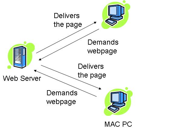

How this works??
The HTTP:TCP transport service uses sockets to transfer the data. The client initiates the TCP connection by using sockets on port 80 to the server. Then the server accepts the connection from the client. The client requests with the HTML pages and the objects which are then exchanged between the client browser and web server. After completing the request, the TCP connection is closed.
As HTTP is a stateless protocol. It does not keep user information about the previous client requests. So, this protocol is simple but if you have to maintain the past client records then it is complex. Since the server will maintain all the client requests and when the server crashes, it is very difficult to get the information back and makes the system very complex.
HTTP Connections
editThe web page consists of objects and URL’s. As there can be one or many objects or URL’s, the type of HTTP connection determines the order in which the objects are requested.
Since the HTTP is constantly evolving to improve its performance, there are two types of connections: • Non-Persistent (HTTP/1.0) • Persistent (HTTP/1.1)
The major difference between non-persistent and persistent connection is the number of TCP connection(s) required for transmitting the objects.
Non-Persistent HTTP – This connection requires that each object be delivered by an individually established TCP connection. Usually there is one round trip time delay for the initial TCP connection. Suppose user requests the page that contains text as well as 5 images. The number of TCP connections will be as follows:


Persistent HTTP -
This connection is also called as HTTP keep-alive, or HTTP Reuse. The idea is to use the same TCP connection to send and receive multiple HTTP requests/responses using the same connection. Using persistent connection is important to improve performance.
Persistent HTTP without Pipelining – In this connection, each client has to wait for the previously requested object received before issuing a new request for another object. Thus, not counting the initial TCP establishment (one RTT time), each object needs at least one RTT plus the transmission time of the object by the server.
Persistent HTTP with Pipelining – Can allow client to send out all (multiple) requests, so servers can receive all requests at once, and then sending responses (objects) one after another. The Pipelining method in HTTP/1.1 is default. The shortest time in pipelining is one initial RTT, RTT for request and response and the transmission time of all the objects by the server.
Thus, we can say that the number of RTT’s required in all the above types considering for some text and three objects would be:
- Non-persistent HTTP:
- Persistent HTTP
- Without Pipelining:
- With Pipelining:
Response Time (Modeling)
editRound Trip Time (RTT): The time taken to send a packet to remote host and receive a response: used to measure delay on the network at a given time.
Response time:
The response time denotes the time required to initiate the TCP connection and the next response and requests to receive back along with the file transmission time.
The following example denotes the response time -


From the above fig. we can state that the response time is :
2 RTT + File transmit time.
HTTP Message Format :
editThere are two types of messages that HTTP uses – 1. Request message 2. Response message
1. Request Message:
editThe request line has three parts, separated by spaces: a method name, the local path of the requested resource and version of HTTP being used. The message format is in ASCII so that it can be read by the humans.
For e.g.:
GET /path/to/the/file.html HTTP/1.0
The GET method is the most commonly used. It states that “give me this resource”. The part of the URL is also called as Request URL. The HTTP is to be in uppercase and the next part denotes the version of HTTP.
HTTP Request Message: General Format
The HTTP Request message format is shown below:
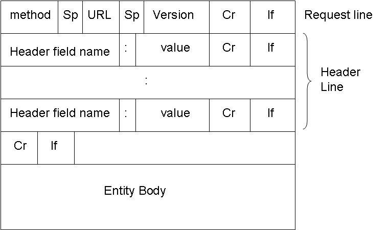

The method is the type of method used to request the URL. Like GET, POST or HEAD. The URL block contains the requested URL. Version denotes the HTTP version. Either HTTP/1.0 or HTTP/1.1. The header lines include the browser type, host , number of objects and file name and the type of language in the requested page. For e.g.:
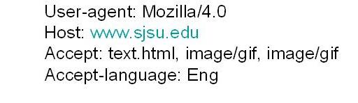

The entity body is used by the POST method. When user enters information on to the page, the entity body contains that information.
The HTTP 1.0 has GET, POST and HEAD methods. While the HTTP 1.1 has along with GET, POST and HEAD, PUT and DELETE.
Uploading the information in Web pages
The POST method
The Web pages which ask for input from user uses the POST method. The information filled by the web user is uploaded in server’s entity body.
The typical form submission in POST method. The content type is usually the application/x-www-form-urlencoded and the content-length is the length of the URL encoded form data.
The URL method
The URL method uses the GET method to get user input from the user. It appends the user information to be uploaded to server to the URL field.
2. Response Message:
editThe HTTP message response line also has three parts separated by spaces: the HTTP version, a response status code giving result of the request and English phrase of the status code. This first line is also called as Status line.
The HTTP Response message format is shown below:
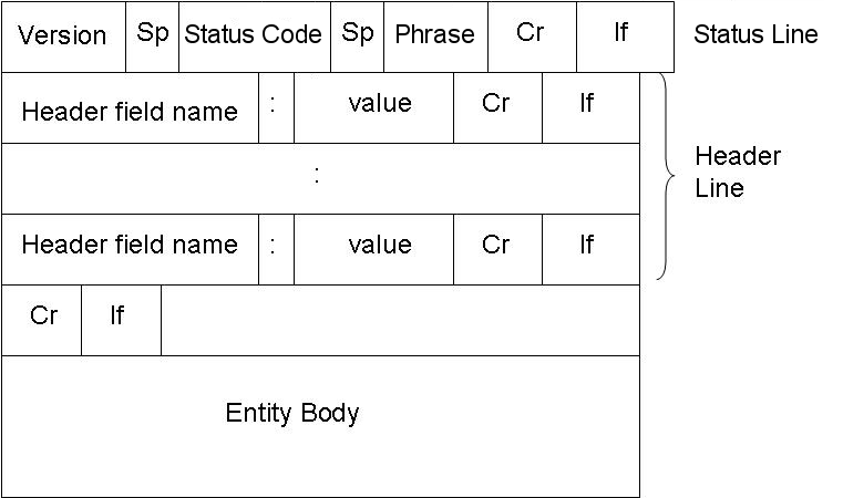

E.g.:
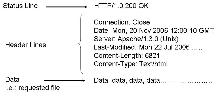

Below are the some HTTP response status codes:
200 OK The request succeeded, and the resulting resource (e.g. file or script output) is returned in the message body.
404 Not Found The requested resource doesn't exist.
301 Moved Permanently
302 Moved Temporarily
303 See Other (HTTP 1.1 only)
The resource has moved to another URL (given by the Location: response header), and should be automatically retrieved by the client. This is often used by a CGI script to redirect the browser to an existing file.
500 Server Error
An unexpected server error. The most common cause is a server-side script that has bad syntax, fails, or otherwise can't run correctly.
User Server Identification
editThe HTTP Protocol is a stateless protocol. So there should be an mechanism to identify the user using the web server. There are various techniques used:
1. Authentication 2. Cookies
1. Authentication:
The Client whenever request for the web page from the web server, the server authenticates the user. So each time whenever the web user or client requests any object, it has to provide a name and password to be identified by server. The need arises for the authentication so that the server has control over the documents. And, Since the HTTP protocol is stateless, it has to provide information each time it requests for web page. The authorization is done at the header line of the request. Generally, the cache is used to store the name and password of the web user. So that, each time it doesn’t have to provide the same information.
2. Cookies
Cookies are used by web servers to identify the web user. They are small piece of data stored into the web users disk. It is used in all major websites. As they have relatively much more importance in the web world. As said earlier, cookie is a small piece of data and not a code. This piece of small information is stored into web users machine whenever the browser visits the server site’s.
So how do the Cookie function exactly?
When the web users browser requests a file from web server, it send the file along with a cookie. So the next time whenever the web browser requests the same server a file, it sends the previous cookie to the web server so that it identifies that the browser had previously requested for a file. And so the web server coordinates your access to different pages from its website.
A typical example can be when you do online shopping., where cookie is used to traced your shopping basket .
The major four component of Cookie are:
1. Cookie header line in the HTTP response message. 2. Cookie header line in the HTTP request message. 3. Cookie file stored in User’s host and managed by User’s browser. 4. Back end database at the web site. So we can say that Cookies are used to keep the State of the web browser. Since HTTP is a stateless, so there should be some means for server to remember the state of the client’s request.
Cookies are in two flavors, one is persistent and the other is non-persistent. Persistent Cookies remain in the web browser’s machine memory for the specified time when it was first created. While non-persistent cookies are the ones which are deleted as soon as the web user’s browser is closed.
Cookies bring a number of useful applications in today’s Internet world. With the help of cookie, you can have: • User accounts • Online Shopping • Web Portals • Advertising
But with these cookies, you can secretly track down the web user’s habits. As whenever a web browser sends a request to web server, it includes its IP address, the type of browser you use and your operating system. So this information is also logged into the server’s file.
The Advertising is the main issue in cookies. Since, it is less admirable because of its use as a tracking of individual’s browsing and buying habits. As the server’s log file has all your information, so it becomes easier to track you. The advertisement firm has many clients which includes another several advertising firms. So it has contracts with many other agencies. They place an image file on their web site. Once you click on them, you are not clicking on the image but a link to another advertising firm’s site. So it sends a cookie to you when you request for that page. And thus, your IP address is tracked down. Whenever you request to their site’s page, they can track your number of visits to their site, which page you have visited and how often. Therefore, they come to know about your interests. So this important piece of information is valuable to them to track your preferences and target you based on your inferences.
Web Caching (Proxy Server)
editThe proxy server’s main goal is to satisfy client’s request without involving the original web server. It is a server acting like as a buffer between the Client’s web browser and the Web server. It accepts the requests from the user and responses to them if it contains the requested page. If it doesn’t have the requested page, then it requests to Original Web Server and responses to the client. It uses cache to store the pages. If the requested web page is in cache, it fulfills the request speedily.
Working of Proxy Server


The two main purpose of proxy server are:
1. Improve Performance –
As it saves the result for a particular period of time. If the same result is requested again and if it is present in the cache of proxy server then the request can be fulfilled in less time. So it drastically improves the performance. The major online searches do have an array of proxy servers to serve for a large number of web users.
2. Filter Requests -
Proxy server’s can also be used to filter requests. Suppose an company wants to restrict the user from accessing a specific set of sites, it can be done with the help of proxy servers.
Conditional GET
The conditional GET is the same as GET method. It only differs by including the If-modified-since, If-unmodified-since, If-match, If-None-Match or If-Range header field. The conditional GET method requests can be satisfied under the given conditions. This is method is used to reduce the network usage so that cache entities can be utilized to fulfill requests if they are not modified and avoids unnecessary transferring of data.
Working of Conditional GET:
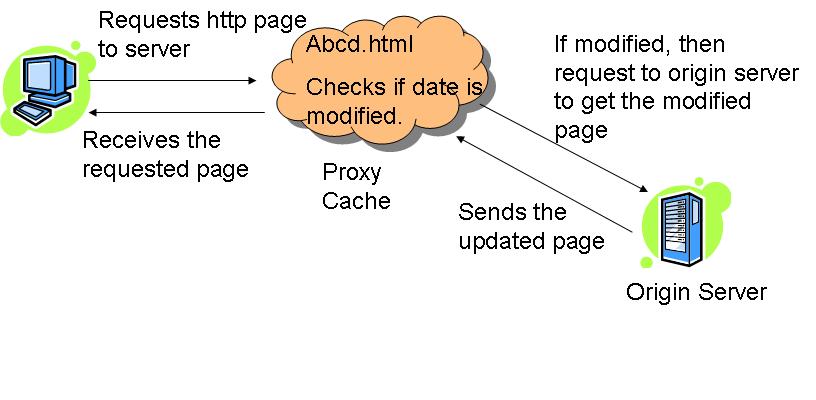

Whenever the client request to the server for html page, the proxy server checks the requested page in its cache. It checks the last-modified date entry in the header


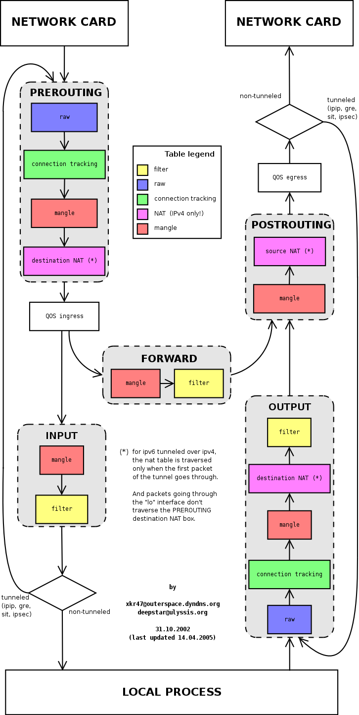
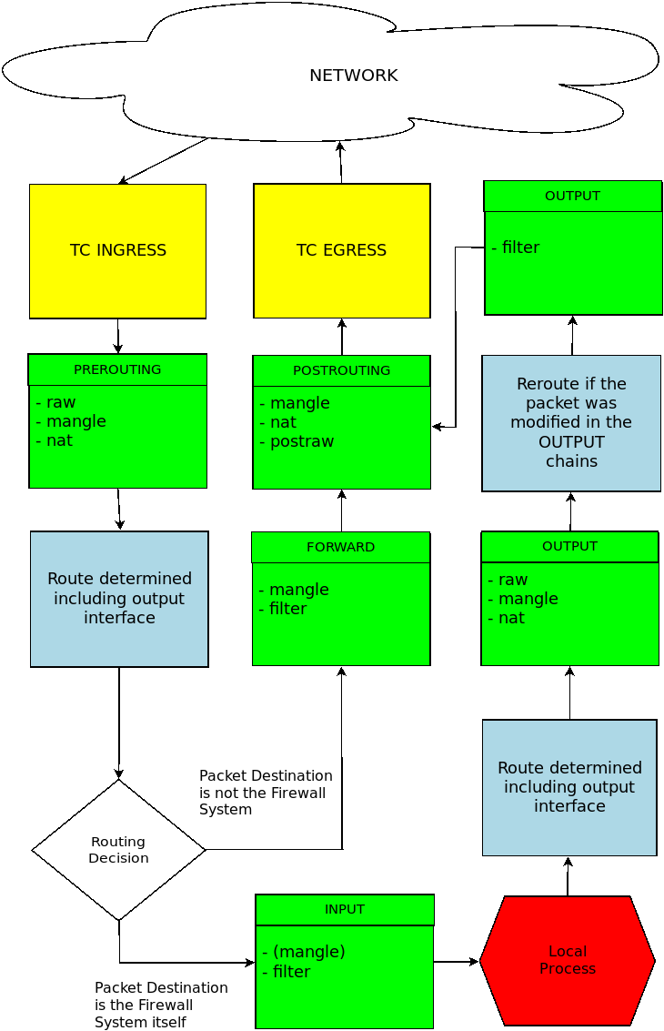
If the requested page in the cache entry determined to be out of date, the proxy server requests the updated page from the main server. And then, the main server responds to that requests and sends updates to the page to the proxy server; which are then forwarded to the client, as well as stored in the proxy server cache.
HTTPS
editThe HTTPS is a secure version of HTTP. It indicates the port 443 should be used instead of port 80. It is widely used, both in security concern areas such as eCommerce, as well as crime prevention by attempting to make sure the end user is actually getting the sites he was looking for. The protocol identifier HTTPS instructs the user agent the user is looking for a secure channel.
The HTTPS follows a procedure to follow secure connection in the network. The secure connection is done automatically. The steps are:
- The client authenticates the server using the server’s digital certificate.
- The client and server negotiate with the cipher suite (a set of security protocols) they will use for the connection.
- The client and server generate session keys for encrypting and decrypting data.
- The Client and server establish a secure encrypted connection.
The HTTPS ends its session whenever the client or server cannot negotiate with the cipher suite. The cipher suite can be based on any of the following:
- Digest Based –
- Message Digest 5 (MD5)
- Secure Hash Algorithm 1 (SHA-1)
- Public Key-Based –
- Rivest-Shamir-Adelman (RSA) encryption/decryption.
- Digital Signature Algorithm (DSA)
- Diffie-Hellman Key-exchange/Key-generation.
- X.509 digital certificates.
SUMMARY
editThis chapter includes HTTP how the Web World is all about. The various methods used in TCP connection to transfer the data in the web world. It has detail information on requests and response methods. Also it contains the User Identification methods like Authentication and Cookies. The cookies part is explained in detail. Also the various connections in HTTP, like non-persistent and persistent connections. We have also mentioned about the proxy server and how does it works. And lastly, the secure version of HTTP.i.e. HTTPS.
Ethereal
Ethereal
editEthereal is a network packet analyzer or a “packet sniffer” as it is called. It was started by Gerald combs in 1997 to track down network problems. Since then Ethereal has been used as the main tool to track and manage network problems and also for R & D purposes.. Ethereal captures network packets from the network during a live network data transmission and gives a detailed summary or description about the packets such as its source and destination, protocols used, packet parameters, network standard, checksum, ports information and much more.
Ethereal is widely used in the networking field as it has many features. some of them are as follows.
- Runs on many platforms such as Windows and Unix.
- Captures live data packets and gives detailed information.
- Saves all the information to be reviewed later.
- Filters packet search on many criteria.
- Supports around 780 protocols.
- Gives detailed summary and statistics after capturing.
- Moreover it is an open software.
And many more.
Ethereal does not detect or troubleshoot the network problems, but it is very important for network management and security as it keeps track of all the packets sent to and fro from your network interface.
Getting started
edit- Getting ethereal
Ethereal is a freeware. Simply download the Ethereal installer from: http://www.ethereal.com/download.html#releases and execute it.
After installing the ethereal package we start it to capture packets. The Ethereal’s Menu options are vast and covers almost all the aspects or options of packet capturing. The basic options of File, Edit, View, etc. have their usual functions. We will go in to the details of the menu afterwards. Let's start capturing packets, because then only you will grasp the real sense of using it. In the menu there is a Capture option. If we click on that button it asks for other options which are essential to both start and customize data capture.
Some of the options under capture tab are:
- Interface: This menu item brings up a dialog box that shows what's going on at the network interfaces Ethereal knows of and we can select our desired interface and capture data on that particular interface.
- Options: This the most important of all the dialog boxes. This menu item brings up the Capture Options dialog box and allows you to start capturing packets. It has all the main options that are required for any packet capturing. It allows you to capture data in promiscuous mode, assign some capture filter, specify capture file where captured packets are to be stored, specify name resolutions and lot lot more. The capture options window is self explanatory and guides you through the various options and gives information about them. The options window is shown below.

Start: It helps to start capturing data immediately with previous settings.
Capture Filters: This menu item brings up a dialog box that allows you to create and edit capture filters which helps you to be more specific with your data capturing.. You can name filters, and you can save them for future use.
After specifying all the options we can start capturing data. when the capturing is stopped then the detailed information is displayed in form of three panes. Which are as follows:
- The Packet List pane: The packet list pane displays all the packets in the current capture file. Each line in the packet list corresponds to one packet in the capture file. If you select a line in this pane, more details will be displayed in the "Packet Details" and "Packet Bytes" panes. This pane gives information regarding the time, destination and source address, protocol used and any other additional information.
- The packet details pane: The packet details pane shows the current packet (selected in the "Packet List" pane) in a more detailed form. This pane shows the protocols and protocol fields of the packet selected in the "Packet List" pane. The protocols and fields of the packet are displayed using a tree, which can be expanded and collapsed
- The packets bytes pane: The packet bytes pane shows the data of the current packet in the hexdump form. When we select some message in the packet list pane, corresponding information is displayed in the other two panes. All types of descriptions on the various topics related to any data capture are provided in these three panes. Let’s explain this by taking an example.
References: http://www.ethereal.com/docs/
Example 1 - Capture of yahoo messenger
editBelow is just an explanation of the ethereal capture of the Yahoo messenger. It takes you through all the basic steps and explains each and every step as detailed as possible.Yahoo messenger use client/server technology for communication. The protocol it uses is yahoo messenger protocol. The yahoo protocol is a application layer protocol, which run over the HTTP and TCP.
Yahoo messenger protocol header
editThe yahoo messenger protocol header is shown below. Each yahoo messenger messages start with the following data format.
| 4 bytes | 4 bytes | 2 bytes | ||
| YMSG | Version | Packet Length | ||
| service | status | session | ||
| Data 0 to 65535 bytes | ||||
HTTP and yahoo messenger protocol header sample
The server acts as a proxy between two clients. All communications between clients go through the server.
Client A < -------------- > server < --------------- > client B
The client and the server both use connection oriented method to establish connection between each other. They use TCP for the same. When the connection is established, they use HTTP protocol to send and receive data. The data portion in the HTTP protocol contain the Yahoo messenger messages. This is decoded by both the server and the client.
When I try to connect to yahoo using yahoo messenger , the following processes happen in the background.
- PC gets the yahoo.com IP address from the DNS server.
- Using the yahoo IP address PC establishes a TCP connection to the yahoo server.
- Then PC sends the yahoo login message through HTTP protocol.
A sample HTTP protocol and yahoo messenger protocol message captured through ethereal is shown below
0000  00 13 10 d4 d7 56 00 0e  9b 7a af 62 08 00 45 00   .....V.. .z.b..E.
0010  02 61 0f 15 40 00 80 06  8b 84 c0 a8 01 ca d8 9b   .a..@... ........
0020  c2 ef 05 6f 00 50 56 bf  09 3e 08 57 9f dd 50 18   ...o.PV. .>.W..P.
0030  ff f0 75 82 00 00 50 4f  53 54 20 2f 6e 6f 74 69   ..u...PO ST /noti
0040  66 79 2f 20 48 54 54 50  2f 31 2e 31 0d 0a 52 65   fy/ HTTP /1.1..Re
;
; other http packets
;
0220  6f 6e 74 72 6f 6c 3a 20  6e 6f 2d 63 61 63 68 65   ontrol:  no-cache
0230  0d 0a 0d 0a 59 4d 53 47  00 0e 00 00 00 25 00 57   ....YMSG .....%.W
0240  00 00 00 00 7a 40 00 00  31 c0 80 70 75 73 75 6b   ....z@.. 1..pusuk
0250  75 c0 80 30 c0 80 70 75  73 75 6b 75 c0 80 32 34   u..0..pu suku..24
0260  c0 80 36 33 35 39 37 39  35 38 32 c0 80 0d 0a      ..635979 582....
The yahoo messenger protocol is the data portion of the HTTP protocol. The yahoo messenger protocol starts with the header YMSG.
| 59 4D 53 47 | YMSG, yahoo messenger protocol message starts |
| 00 0e 00 00 | Version, yahoo messenger version is 14 |
| 00 25 | Length, packet length 37 bytes or 0x25 bytes |
| 00 57 | Yahoo Service, service in this case is YAHOO_SERVICE_AUTH |
| 00 00 00 00 | Yahoo Status , Status of the using trying to login in this case is YAHOO_STATUS_AVAILABLE |
| 7a 40 00 00 | Yahoo Session ID, Session id of the client and server. Followed by the data |
Yahoo messenger protocol background process using ethereal The following explains a simple communication between the yahoo client and yahoo server . In this case client A send a message to client B, where client B is offline. Each process is explained with packet capture using ethereal.
Login process
edit- Client A log in to yahoo messenger.
1. When client A submits the login button of the yahoo messenger with his user id and password the following happens between the client ( Client A yahoo messenger) and yahoo server. Client A says I want to login as <username> here is the session id ‘7a 40 00 00’ and user name pusuku
0230   0d 0a 0d 0a 59 4d 53 47 00 0e 00 00 00 25 00 57  ....YMSG.....%.W
0240   00 00 00 00 7a 40 00 00 31 c0 80 70 75 73 75 6b  ....z@..1..pusuk
0250   75 c0 80 30 c0 80 70 75 73 75 6b 75 c0 80 32 34  u..0..pusuku..24
0260   c0 80 36 33 35 39 37 39 35 38 32 c0 80 0d 0a     ..635979582....
7a 40 00 00 is the session id, Client sents a YAHOO_SERVICE_AUTH (00 57) with status YAHOO_STATUS_AVAILABLE(00 00 00 00)
2. Server responds , Okay , Here is a challenge string , Using this to hash your id and password and send it to me
0170   00 00 59 4d 53 47 00 00 00 00 00 59 00 57 00 00  ..YMSG.....Y.W..
0180   00 01 7a 40 00 00 31 c0 80 70 75 73 75 6b 75 c0  ..z@..1..pusuku.
0190   80 39 34 c0 80 64 7c 67 2d 75 5e 77 2f 79 2d 72  .94..d|g-u^w/y-r
01a0   2b 38 2b 70 2a 6b 2a 7a 2f 61 2d 35 2b 33 2a 62  +8+p*k*z/a-5+3*b
01b0   26 68 25 32 2a 75 2f 6e 2f 28 77 2d 70 2d 75 25  &h%2*u/n/(w-p-u%
01c0   71 2a 76 7c 7a 2a 6e 25 66 2f 67 2a 6e 7c 74 25  q*v|z*n%f/g*n|t%
01d0   79 26 6d 26 6d 29 c0 80 31 33 c0 80 32 c0 80     y&m&m)..13..2..
Server responds with YAHOO_SERVICE_AUTH (00 57) and status YaHOO_STATUS_BRB and the challenge string in the data portion of the yahoo messenger protocol
3. Client says, here is the user id and password hashed with the challenge string
01f0   6c 3a 20 6e 6f 2d 63 61 63 68 65 0d 0a 0d 0a 59  l: no-cache....Y
0200   4d 53 47 00 0e 00 00 03 2f 00 54 00 00 00 0c 7a  MSG...../.T....z
;
; other hashed messages
;
0540   c0 80 0d 0a                                      ....
Client sends a YAHOO_SERVICE_AUTHRESP (00 54) with user and password hashed with the challenge string , The hashed challenge string is sent as data portion
4. Server verifies the user id and password and responds , okay your authenticated , here is your buddy list
0170   00 00 59 4d 53 47 00 00 00 00 03 c7 00 55 00 00  ..YMSG.......U..
0180   00 05 7a 40 00 00 38 37 c0 80 43 68 61 74 20 46  ..z@..87..Chat F
0190   72 69 65 6e 64 73 3a 63 6c 75 6d 73 79 64 72 65  riends:clumsydre
01a0   61 6d 73 2c 64 75 72 67 61 6b 73 2c 6b 69 72 75  ams,durgaks,kiru
;
; other buddy list and their status
;
0510   31 38 35 c0 80 63 6c 75 6d 73 79 64 72 65 61 6d  185..clumsydream
0520   73 2c                                            s,
Server on authentication responds with the buddy list YAHOO_SERVICE_LIST (00 55) With this Client A is ready is ready to send the message to Client B , Tough client A knows , Client B is offline client A sends a offline message .
Send process
editAs Client A select Client B window and start typing, 1. The Client says , I am typing message for my buddy
0230   0d 0a 0d 0a 59 4d 53 47 00 0e 00 00 00 4a 00 4b  ....YMSG.....J.K
0240   00 00 00 16 7a 40 00 00 34 39 c0 80 54 59 50 49  ....z@..49..TYPI
0250   4e 47 c0 80 31 c0 80 70 75 73 75 6b 75 c0 80 31  NG..1..pusuku..1
0260   34 c0 80 20 c0 80 31 33 c0 80 31 c0 80 35 c0 80  4.. ..13..1..5..
0270   64 73 75 73 61 69 c0 80 30 c0 80 70 75 73 75 6b  dnunai..0..pusuk
0280   75 c0 80 32 34 c0 80 32 31 33 31 30 33 33 39 33  u..24..213103393
0290   c0 80 0d 0a                                      ....
client sends YAHOO_SERVICE_NOTIFY(00 4b) message saying pusuku is sending message to dnunai with the status YAHOO_SERVICE_TYPING (0x16)
2. When the user presses the send button . The client sends the message to the server client send this message <msg> to my buddy <buddyname> server
0230   65 0d 0a 0d 0a 59 4d 53 47 00 0e 00 00 00 5c 00  e....YMSG.....\.
0240   06 5a 55 aa 56 7a 40 00 00 31 c0 80 70 75 73 75  .ZU.Vz@..1..pusu
0250   6b 75 c0 80 35 c0 80 64 73 75 73 61 69 c0 80 31  ku..5..dnunai..1
0260   34 c0 80 68 69 20 64 65 6c 6c 61 c0 80 39 37 c0  4..hi kella..97.
0270   80 31 c0 80 36 33 c0 80 3b 30 c0 80 36 34 c0 80  .1..63..;0..64..
0280   30 c0 80 32 30 36 c0 80 32 c0 80 30 c0 80 70 75  0..206..2..0..pu
0290   73 75 6b 75 c0 80 32 34 c0 80 32 31 33 31 30 33  suku..24..213103
02a0   33 39 33 c0 80 0d 0a                             393....
client sends YAHOO_SERVICE_MESSAGE(00 06) message to the server The server processes the message , The message is from pusuku to dnunai(who’s status is offline, 5a 55 aa 56) Note the message sent ‘ hi kella’ Since Client B is offline , the server stores the message and sends it to client B , when client B log in. Now, client A has sent the message, time to logout.
Logout process
edit1. Client A says , I am done , I am logging out .
0230   0d 0a 0d 0a 59 4d 53 47 00 0e 00 00 00 1a 00 02  ....YMSG........
0240   00 00 00 00 7a 40 00 00 30 c0 80 50 55 53 55 4b  ....z@..0..PUSUK
0250   55 c0 80 32 34 c0 80 32 31 33 31 30 33 33 39 33  U..24..213103393
0260   c0 80 0d 0a                                      ....
client sends YAHOO_SERVICE_LOGOFF(00 02) message to server
2. Server responds , okay .
0170   00 00 59 4d 53 47 00 00 00 00 00 00 00 02 00 00  ..YMSG..........
0180   00 00 7a 40 00 00                                ..z@..
Server responds with empty message with service YAHOO_SERVICE_LOGOFF
Understanding Tracert with Ethereal
editTracert is a windows based tool for tracing the path of the packets taken from your pc to the destination router. This assignment traces the path from my pc to www.yahoo.com using Tracert
C:\DOCUME~1\skva>tracert www.yahoo.com

Tracing route to www.yahoo-ht2.akadns.net [209.131.36.158]
over a maximum of 30 hops:

  1     1 ms     1 ms     1 ms  c-24-6-102-212.hsd1.ca.comcast.net [24.6.102.212]
  2     *        *        *     Request timed out.
  3    11 ms     *        *     GE-2-1-ur01.santaclara.ca.sfba.comcast.net [68.87.198.105]
  4    11 ms    11 ms     *     10g-9-3-ur02.santaclara.ca.sfba.comcast.net [68.87.192.26]
  5    14 ms     *       12 ms  10g-9-4-ar01.oakland.ca.sfba.comcast.net [68.87.192.34]
  6     *        *        *     Request timed out.
  7    13 ms    14 ms    12 ms  12.118.38.5
  8    13 ms    14 ms    17 ms  tbr1-p010802.sffca.ip.att.net [12.123.12.66]
  9    14 ms    14 ms    11 ms  ggr2-p310.sffca.ip.att.net [12.123.12.18]
 10    15 ms    15 ms    14 ms  att-gw.sea.level3.net [192.205.32.206]
 11    16 ms    14 ms    14 ms  4.71.112.14
 12    15 ms    16 ms    17 ms  g-1-0-0-p171.msr2.sp1.yahoo.com [216.115.107.87]
 13    16 ms    16 ms    16 ms  te-8-1.bas-a1.sp1.yahoo.com [209.131.32.17]
 14    19 ms    17 ms    17 ms  f1.www.vip.sp1.yahoo.com [209.131.36.158]

Trace complete.
The above output from tracert shows the number of routes it took, name of the routers on the way and time taken to reach each router. It took 14 hops to reach the yahoo server from my pc. The asterisk indicate the failed attempt for next route.
When I executed the command ‘tracert www.yahoo.com’ the following happens in the back ground. The packets were captured using ethereal.
Step 1: The PC sends a DNS request to the DNS server to resolve the ip address of yahoo.com.
192.168.1.101 to 68.87.76.178 DNS standard query A www.yahoo.com
68.87.76.178 to 192.168.1.101 DNS standard query response CNAME
                              www.yahoo-ht2.akadns.net Address 209.131.36.158
Step 2: After getting yahoo.com ip address , tracert sends icmp echo request message with TTL set to 1, Each echo request is received by the router at the first hop , which responds with ‘time to live exceeded live‘ message. Each hop packets are analyzed below .
Hop 1
edit1 1 ms 1 ms 1 ms c-24-6-102-212.hsd1.ca.comcast.net [24.6.102.212] Echo request packets were sent with TTL set to 1 0000 00 13 10 d4 d7 56 00 0e 9b 7a af 62 08 00 45 00 .....V...z.b..E. 0010 00 5c a8 f9 00 00 01 01 58 79 c0 a8 01 65 d1 83 .\......Xy...e.. 0020 24 9e 08 00 f4 ff 02 00 01 00 00 00 00 00 00 00 $............... 0030 00 00 00 00 00 00 00 00 00 00 00 00 00 00 00 00 ................ 0040 00 00 00 00 00 00 00 00 00 00 00 00 00 00 00 00 ................ 0050 00 00 00 00 00 00 00 00 00 00 00 00 00 00 00 00 ................ 0060 00 00 00 00 00 00 00 00 00 00 ..........
| 45 | = IP version 4 |
| 01 | = TTL (time to live ) |
| 01 | = ICMP protocol |
| c0 a8 01 65 | = Source ip address = > 192.168.1.101 |
| d1 83 24 9e | = Destination ip address = > 209.131.36.158 |
| 08 | = Type 8 ICMP (Echo (ping) request) |
| 00 | = Code , net unreachable |
0000   00 0e 9b 7a af 62 00 13 10 d4 d7 56 08 00 45 4f  ...z.b.....V..EO
0010   00 38 0a 93 00 00 40 01 2e fc 18 06 66 d4 c0 a8  .8....@.....f...
0020   01 65 0b 00 f4 ff 00 00 00 00 45 00 00 5c a8 f9  .e........E..\..
0030   00 00 01 01 58 79 c0 a8 01 65 d1 83 24 9e 08 00  ....Xy...e..$...
0040   f4 ff 02 00 01 00                                ......
| 45 | = IP version 4 |
| 40 | = TTL (time to live ) => 64 |
| 01 | = ICMP protocol |
| 18 06 66 d4 | = Source ip address = > 24.6.102.212 |
| C0 a8 01 65 | = Destination ip address = > 192.168.1.101 |
| 0b | = Type ICMP => 11 (time to live exceeded |
| 00 | = Code , net unreachable (time to live exceeded in transit) |
0000   00 13 10 d4 d7 56 00 0e 9b 7a af 62 08 00 45 00  .....V...z.b..E.
0010   00 5c a8 fa 00 00 01 01 58 78 c0 a8 01 65 d1 83  .\......Xx...e..
0020   24 9e 08 00 f3 ff 02 00 02 00 00 00 00 00 00 00  $...............
0030   00 00 00 00 00 00 00 00 00 00 00 00 00 00 00 00  ................
0040   00 00 00 00 00 00 00 00 00 00 00 00 00 00 00 00  ................
0050   00 00 00 00 00 00 00 00 00 00 00 00 00 00 00 00  ................
0060   00 00 00 00 00 00 00 00 00 00                    ..........
| 45 | = IP version 4 |
| 01 | = TTL (time to live ) |
| 01 | = ICMP protocol |
| c0 a8 01 65 | = Source ip address = > 192.168.1.101 |
| d1 83 24 9e | = Destination ip address = > 209.131.36.158 |
| 08 | = Type 8 ICMP (Echo (ping) request) |
| 00 | = Code , net unreachable |
0000   00 0e 9b 7a af 62 00 13 10 d4 d7 56 08 00 45 4f  ...z.b.....V..EO
0010   00 38 0a 94 00 00 40 01 2e fb 18 06 66 d4 c0 a8  .8....@.....f...
0020   01 65 0b 00 f2 ff 00 00 00 00 45 00 00 5c a8 fa  .e........E..\..
0030   00 00 01 01 58 78 c0 a8 01 65 d1 83 24 9e 08 00  ....Xx...e..$...
0040   f3 ff 02 00 02 00                                ......
| 45 | = IP version 4 |
| 40 | = TTL (time to live ) => 64 |
| 01 | = ICMP protocol |
| 18 06 66 d4 | = Source ip address = > 24.6.102.212 |
| C0 a8 01 65 | = Destination ip address = > 192.168.1.101 |
| 0b | = Type ICMP (Echo (ping) request) => 11 (time to live exceeded |
| 00 | = Code , net unreachable (time to live exceeded in transit) |
0000   00 13 10 d4 d7 56 00 0e 9b 7a af 62 08 00 45 00  .....V...z.b..E.
0010   00 5c a8 fa 00 00 01 01 58 78 c0 a8 01 65 d1 83  .\......Xx...e..
0020   24 9e 08 00 f3 ff 02 00 02 00 00 00 00 00 00 00  $...............
0030   00 00 00 00 00 00 00 00 00 00 00 00 00 00 00 00  ................
0040   00 00 00 00 00 00 00 00 00 00 00 00 00 00 00 00  ................
0050   00 00 00 00 00 00 00 00 00 00 00 00 00 00 00 00  ................
0060   00 00 00 00 00 00 00 00 00 00                    ..........
| 45 | = IP version 4 |
| 01 | = TTL (time to live ) |
| 01 | = ICMP protocol |
| c0 a8 01 65 | = Source ip address = > 192.168.1.101 |
| d1 83 24 9e | = Destination ip address = > 209.131.36.158 |
| 08 | = Type 8 ICMP (Echo (ping) request) |
| 00 | = Code , net unreachable |
0000   00 0e 9b 7a af 62 00 13 10 d4 d7 56 08 00 45 4f  ...z.b.....V..EO
0010   00 38 0a 94 00 00 40 01 2e fb 18 06 66 d4 c0 a8  .8....@.....f...
0020   01 65 0b 00 f4 ff 00 00 00 00 45 00 00 5c a8 fa  .e........E..\..
0030   00 00 01 01 58 78 c0 a8 01 65 d1 83 24 9e 08 00  ....Xx...e..$...
0040   f3 ff 02 00 02 00                                ......
| 45 | = IP version 4 |
| 40 | = TTL (time to live ) => 64 |
| 01 | = ICMP protocol |
| 18 06 66 d4 | = Source ip address = > 24.6.102.212 |
| C0 a8 01 65 | = Destination ip address = > 192.168.1.101 |
| 0b | = Type ICMP (Echo (ping) request) => 11 (time to live exceeded |
| 00 | = Code , net unreachable (time to live exceeded in transit) |
Hop 2
edit2 * * * Request timed out. Echo request packets were sent with TTL set to 2 0000 00 13 10 d4 d7 56 00 0e 9b 7a af 62 08 00 45 00 .....V...z.b..E. 0010 00 5c a9 01 00 00 02 01 57 71 c0 a8 01 65 d1 83 .\......Wq...e.. 0020 24 9e 08 00 f1 ff 02 00 04 00 00 00 00 00 00 00 $............... 0030 00 00 00 00 00 00 00 00 00 00 00 00 00 00 00 00 ................ 0040 00 00 00 00 00 00 00 00 00 00 00 00 00 00 00 00 ................ 0050 00 00 00 00 00 00 00 00 00 00 00 00 00 00 00 00 ................ 0060 00 00 00 00 00 00 00 00 00 00 ..........
| 45 | = IP version 4 |
| 02 | = TTL (time to live ) => 2 |
| 01 | = ICMP protocol |
| c0 a8 01 65 | = Source ip address = > 192.168.1.101 |
| d1 83 24 9e | = Destination ip address = > 209.131.36.158 |
| 08 | = Type 8 ICMP (Echo (ping) request) |
| 00 | = Code , net unreachable |
0000   00 13 10 d4 d7 56 00 0e 9b 7a af 62 08 00 45 00  .....V...z.b..E.
0010   00 5c a9 01 00 00 02 01 57 71 c0 a8 01 65 d1 83  .\......Wq...e..
0020   24 9e 08 00 f1 ff 02 00 04 00 00 00 00 00 00 00  $...............
0030   00 00 00 00 00 00 00 00 00 00 00 00 00 00 00 00  ................
0040   00 00 00 00 00 00 00 00 00 00 00 00 00 00 00 00  ................
0050   00 00 00 00 00 00 00 00 00 00 00 00 00 00 00 00  ................
0060   00 00 00 00 00 00 00 00 00 00                    ..........
| 45 | = IP version 4 |
| 02 | = TTL (time to live ) => 2 |
| 01 | = ICMP protocol |
| c0 a8 01 65 | = Source ip address = > 192.168.1.101 |
| d1 83 24 9e | = Destination ip address = > 209.131.36.158 |
| 08 | = Type 8 ICMP (Echo (ping) request) |
| 00 | = Code , net unreachable |
Hop 3
edit3 11 ms * * GE-2-1-ur01.santaclara.ca.sfba.comcast.net [68.87.198.105] Echo request packets were sent with TTL set to 3 0000 00 13 10 d4 d7 56 00 0e 9b 7a af 62 08 00 45 00 .....V...z.b..E. 0010 00 5c a9 41 00 00 03 01 56 31 c0 a8 01 65 d1 83 .\.A....V1...e.. 0020 24 9e 08 00 ee ff 02 00 07 00 00 00 00 00 00 00 $............... 0030 00 00 00 00 00 00 00 00 00 00 00 00 00 00 00 00 ................ 0040 00 00 00 00 00 00 00 00 00 00 00 00 00 00 00 00 ................ 0050 00 00 00 00 00 00 00 00 00 00 00 00 00 00 00 00 ................ 0060 00 00 00 00 00 00 00 00 00 00 ..........
| 45 | = IP version 4 |
| 03 | = TTL (time to live ) => 3 |
| 01 | = ICMP protocol |
| c0 a8 01 65 | = Source ip address = > 192.168.1.101 |
| d1 83 24 9e | = Destination ip address = > 209.131.36.158 |
| 08 | = Type 8 ICMP (Echo (ping) request) |
| 00 | = Code , net unreachable |
0000   00 0e 9b 7a af 62 00 13 10 d4 d7 56 08 00 45 c0  ...z.b.....V..E.
0010   00 38 23 76 00 00 fd 01 cc c0 44 57 c6 69 c0 a8  .8#v......DW.i..
0020   01 65 0b 00 f4 ff 00 00 00 00 45 20 00 5c a9 41  .e........E .\.A
0030   00 00 01 01 58 11 c0 a8 01 65 d1 83 24 9e 08 00  ....X....e..$...
0040   ee ff 02 00 07 00                                ......
| 45 | = IP version 4 |
| fd | = TTL (time to live ) => 253 |
| 01 | = ICMP protocol |
| 44 57 c6 69 | = Source ip address = > 68.87.198.105 |
| a8 01 65 | = Destination ip address = > 192.168.1.101 |
| 0b | = Type ICMP (Echo (ping) request) => 11 (time to live exceeded |
| 00 | = Code , net unreachable (time to live exceeded in transit) |
0000   00 13 10 d4 d7 56 00 0e 9b 7a af 62 08 00 45 00  .....V...z.b..E.
0010   00 5c a9 42 00 00 03 01 56 30 c0 a8 01 65 d1 83  .\.B....V0...e..
0020   24 9e 08 00 ed ff 02 00 08 00 00 00 00 00 00 00  $...............
0030   00 00 00 00 00 00 00 00 00 00 00 00 00 00 00 00  ................
0040   00 00 00 00 00 00 00 00 00 00 00 00 00 00 00 00  ................
0050   00 00 00 00 00 00 00 00 00 00 00 00 00 00 00 00  ................
0060   00 00 00 00 00 00 00 00 00 00                    ..........
| 45 | = IP version 4 |
| 03 | = TTL (time to live ) => 3 |
| 01 | = ICMP protocol |
| c0 a8 01 65 | = Source ip address = > 192.168.1.101 |
| d1 83 24 9e | = Destination ip address = > 209.131.36.158 |
| 08 | = Type 8 ICMP (Echo (ping) request) |
| 00 | = Code, net unreachable |
0000   00 13 10 d4 d7 56 00 0e 9b 7a af 62 08 00 45 00  .....V...z.b..E.
0010   00 5c a9 59 00 00 03 01 56 19 c0 a8 01 65 d1 83  .\.Y....V....e..
0020   24 9e 08 00 ec ff 02 00 09 00 00 00 00 00 00 00  $...............
0030   00 00 00 00 00 00 00 00 00 00 00 00 00 00 00 00  ................
0040   00 00 00 00 00 00 00 00 00 00 00 00 00 00 00 00  ................
0050   00 00 00 00 00 00 00 00 00 00 00 00 00 00 00 00  ................
0060   00 00 00 00 00 00 00 00 00 00                    ..........
| 45 | = IP version 4 |
| 03 | = TTL (time to live ) => 3 |
| 01 | = ICMP protocol |
| c0 a8 01 65 | = Source ip address = > 192.168.1.101 |
| d1 83 24 9e | = Destination ip address = > 209.131.36.158 |
| 08 | = Type 8 ICMP (Echo (ping) request) |
| 00 | = Code, net unreachable |
Hop 4
edit4 11 ms 11 ms * 10g-9-3-ur02.santaclara.ca.sfba.comcast.net [68.87.192.26] Echo request packets were sent with TTL set to 4 0000 00 13 10 d4 d7 56 00 0e 9b 7a af 62 08 00 45 00 .....V...z.b..E. 0010 00 5c a9 6c 00 00 04 01 55 06 c0 a8 01 65 d1 83 .\.l....U....e.. 0020 24 9e 08 00 eb ff 02 00 0a 00 00 00 00 00 00 00 $............... 0030 00 00 00 00 00 00 00 00 00 00 00 00 00 00 00 00 ................ 0040 00 00 00 00 00 00 00 00 00 00 00 00 00 00 00 00 ................ 0050 00 00 00 00 00 00 00 00 00 00 00 00 00 00 00 00 ................ 0060 00 00 00 00 00 00 00 00 00 00 ..........
| 45 | = IP version 4 |
| 04 | = TTL (time to live ) => 4 |
| 01 | = ICMP protocol |
| c0 a8 01 65 | = Source ip address = > 192.168.1.101 |
| d1 83 24 9e | = Destination ip address = > 209.131.36.158 |
| 08 | = Type 8 ICMP (Echo (ping) request) |
| 00 | = Code, net unreachable |
0000   00 0e 9b 7a af 62 00 13 10 d4 d7 56 08 00 45 c0  ...z.b.....V..E.
0010   00 38 6e 22 00 00 fd 01 88 63 44 57 c0 1a c0 a8  .8n".....cDW....
0020   01 65 0b 00 f4 ff 00 00 00 00 45 20 00 5c a9 6c  .e........E .\.l
0030   00 00 01 01 57 e6 c0 a8 01 65 d1 83 24 9e 08 00  ....W....e..$...
0040   eb ff 02 00 0a 00                                ......
| 45 | = IP version 4 |
| fd | = TTL (time to live ) => 253 |
| 01 | = ICMP protocol |
| 44 57 c0 1a | = Source ip address = > 68.87.192.26 |
| c0 a8 01 65 | = Destination ip address = > 192.168.1.101 |
| 0b | = Type ICMP (Echo (ping) request) => 11 (time to live exceeded |
| 00 | = Code , net unreachable (time to live exceeded in transit) |
0000   00 13 10 d4 d7 56 00 0e 9b 7a af 62 08 00 45 00  .....V...z.b..E.
0010   00 5c a9 6d 00 00 04 01 55 05 c0 a8 01 65 d1 83  .\.m....U....e..
0020   24 9e 08 00 ea ff 02 00 0b 00 00 00 00 00 00 00  $...............
0030   00 00 00 00 00 00 00 00 00 00 00 00 00 00 00 00  ................
0040   00 00 00 00 00 00 00 00 00 00 00 00 00 00 00 00  ................
0050   00 00 00 00 00 00 00 00 00 00 00 00 00 00 00 00  ................
0060   00 00 00 00 00 00 00 00 00 00                    ..........
| 45 | = IP version 4 |
| 04 | = TTL (time to live ) => 4 |
| 01 | = ICMP protocol |
| c0 a8 01 65 | = Source ip address = > 192.168.1.101 |
| d1 83 24 9e | = Destination ip address = > 209.131.36.158 |
| 08 | = Type 8 ICMP (Echo (ping) request) |
| 00 | = Code, net unreachable |
0000   00 0e 9b 7a af 62 00 13 10 d4 d7 56 08 00 45 c0  ...z.b.....V..E.
0010   00 38 6e 23 00 00 fd 01 88 62 44 57 c0 1a c0 a8  .8n#.....bDW....
0020   01 65 0b 00 f4 ff 00 00 00 00 45 20 00 5c a9 6d  .e........E .\.m
0030   00 00 01 01 57 e5 c0 a8 01 65 d1 83 24 9e 08 00  ....W....e..$...
0040   ea ff 02 00 0b 00                                ......
| 45 | = IP version 4 |
| fd | = TTL (time to live ) => 253 |
| 01 | = ICMP protocol |
| 44 57 c0 1a | = Source ip address = > 68.87.192.26 |
| c0 a8 01 65 | = Destination ip address = > 192.168.1.101 |
| 0b | = Type ICMP (Echo (ping) request) => 11 (time to live exceeded |
| 00 | = Code , net unreachable (time to live exceeded in transit) |
0000   00 13 10 d4 d7 56 00 0e 9b 7a af 62 08 00 45 00  .....V...z.b..E.
0010   00 5c a9 6e 00 00 04 01 55 04 c0 a8 01 65 d1 83  .\.n....U....e..
0020   24 9e 08 00 e9 ff 02 00 0c 00 00 00 00 00 00 00  $...............
0030   00 00 00 00 00 00 00 00 00 00 00 00 00 00 00 00  ................
0040   00 00 00 00 00 00 00 00 00 00 00 00 00 00 00 00  ................
0050   00 00 00 00 00 00 00 00 00 00 00 00 00 00 00 00  ................
0060   00 00 00 00 00 00 00 00 00 00                    ..........
| 45 | = IP version 4 |
| 04 | = TTL (time to live ) => 4 |
| 01 | = ICMP protocol |
| c0 a8 01 65 | = Source ip address = > 192.168.1.101 |
| d1 83 24 9e | = Destination ip address = > 209.131.36.158 |
| 08 | = Type 8 ICMP (Echo (ping) request) |
| 00 | = Code, net unreachable |
Hop 5
edit5 14 ms * 12 ms 10g-9-4-ar01.oakland.ca.sfba.comcast.net [68.87.192.34] Echo request packets were sent with TTL set to 5 0000 00 13 10 d4 d7 56 00 0e 9b 7a af 62 08 00 45 00 .....V...z.b..E. 0010 00 5c a9 89 00 00 05 01 53 e9 c0 a8 01 65 d1 83 .\......S....e.. 0020 24 9e 08 00 e8 ff 02 00 0d 00 00 00 00 00 00 00 $............... 0030 00 00 00 00 00 00 00 00 00 00 00 00 00 00 00 00 ................ 0040 00 00 00 00 00 00 00 00 00 00 00 00 00 00 00 00 ................ 0050 00 00 00 00 00 00 00 00 00 00 00 00 00 00 00 00 ................ 0060 00 00 00 00 00 00 00 00 00 00 ..........
| 45 | = IP version 4 |
| 05 | = TTL (time to live ) => 5 |
| 01 | = ICMP protocol |
| c0 a8 01 65 | = Source ip address = > 192.168.1.101 |
| d1 83 24 9e | = Destination ip address = > 209.131.36.158 |
| 08 | = Type 8 ICMP (Echo (ping) request) |
| 00 | = Code, net unreachable |
0000   00 0e 9b 7a af 62 00 13 10 d4 d7 56 08 00 45 c0  ...z.b.....V..E.
0010   00 38 fa 4e 00 00 fc 01 fd 2e 44 57 c0 22 c0 a8  .8.N......DW."..
0020   01 65 0b 00 f4 ff 00 00 00 00 45 20 00 5c a9 89  .e........E .\..
0030   00 00 01 01 57 c9 c0 a8 01 65 d1 83 24 9e 08 00  ....W....e..$...
0040   e8 ff 02 00 0d 00                                ......
| 45 | = IP version 4 |
| fd | = TTL (time to live ) => 252 |
| 01 | = ICMP protocol |
| 44 57 c0 22 | = Source ip address = > 68.87.192.34 |
| c0 a8 01 65 | = Destination ip address = > 192.168.1.101 |
| 0b | = Type ICMP (Echo (ping) request) => 11 (time to live exceeded |
| 00 | = Code , net unreachable (time to live exceeded in transit) |
0000   00 13 10 d4 d7 56 00 0e 9b 7a af 62 08 00 45 00  .....V...z.b..E.
0010   00 5c a9 8a 00 00 05 01 53 e8 c0 a8 01 65 d1 83  .\......S....e..
0020   24 9e 08 00 e7 ff 02 00 0e 00 00 00 00 00 00 00  $...............
0030   00 00 00 00 00 00 00 00 00 00 00 00 00 00 00 00  ................
0040   00 00 00 00 00 00 00 00 00 00 00 00 00 00 00 00  ................
0050   00 00 00 00 00 00 00 00 00 00 00 00 00 00 00 00  ................
0060   00 00 00 00 00 00 00 00 00 00                    ..........
| 45 | = IP version 4 |
| 05 | = TTL (time to live ) => 5 |
| 01 | = ICMP protocol |
| c0 a8 01 65 | = Source ip address = > 192.168.1.101 |
| d1 83 24 9e | = Destination ip address = > 209.131.36.158 |
| 08 | = Type 8 ICMP (Echo (ping) request) |
| 00 | = Code, net unreachable |
0000   00 13 10 d4 d7 56 00 0e 9b 7a af 62 08 00 45 00  .....V...z.b..E.
0010   00 5c a9 9f 00 00 05 01 53 d3 c0 a8 01 65 d1 83  .\......S....e..
0020   24 9e 08 00 e6 ff 02 00 0f 00 00 00 00 00 00 00  $...............
0030   00 00 00 00 00 00 00 00 00 00 00 00 00 00 00 00  ................
0040   00 00 00 00 00 00 00 00 00 00 00 00 00 00 00 00  ................
0050   00 00 00 00 00 00 00 00 00 00 00 00 00 00 00 00  ................
0060   00 00 00 00 00 00 00 00 00 00                    ..........
| 45 | = IP version 4 |
| 05 | = TTL (time to live ) => 5 |
| 01 | = ICMP protocol |
| c0 a8 01 65 | = Source ip address = > 192.168.1.101 |
| d1 83 24 9e | = Destination ip address = > 209.131.36.158 |
| 08 | = Type 8 ICMP (Echo (ping) request) |
| 00 | = Code, net unreachable |
0000   00 0e 9b 7a af 62 00 13 10 d4 d7 56 08 00 45 c0  ...z.b.....V..E.
0010   00 38 fc 75 00 00 fc 01 fb 07 44 57 c0 22 c0 a8  .8.u......DW."..
0020   01 65 0b 00 f4 ff 00 00 00 00 45 20 00 5c a9 9f  .e........E .\..
0030   00 00 01 01 57 b3 c0 a8 01 65 d1 83 24 9e 08 00  ....W....e..$...
0040   e6 ff 02 00 0f 00                                ......
| 45 | = IP version 4 |
| fd | = TTL (time to live ) => 252 |
| 01 | = ICMP protocol |
| 44 57 c0 22 | = Source ip address = > 68.87.192.34 |
| c0 a8 01 65 | = Destination ip address = > 192.168.1.101 |
| 0b | = Type ICMP (Echo (ping) request) => 11 (time to live exceeded |
| 00 | = Code , net unreachable (time to live exceeded in transit) |
Hop 6
edit6 * * * Request timed out. Echo request packets were sent with TTL set to 6 0000 00 13 10 d4 d7 56 00 0e 9b 7a af 62 08 00 45 00 .....V...z.b..E. 0010 00 5c a9 a5 00 00 06 01 52 cd c0 a8 01 65 d1 83 .\......R....e.. 0020 24 9e 08 00 e5 ff 02 00 10 00 00 00 00 00 00 00 $............... 0030 00 00 00 00 00 00 00 00 00 00 00 00 00 00 00 00 ................ 0040 00 00 00 00 00 00 00 00 00 00 00 00 00 00 00 00 ................ 0050 00 00 00 00 00 00 00 00 00 00 00 00 00 00 00 00 ................ 0060 00 00 00 00 00 00 00 00 00 00 ..........
| 45 | = IP version 4 |
| 06 | = TTL (time to live ) => 6 |
| 01 | = ICMP protocol |
| c0 a8 01 65 | = Source ip address = > 192.168.1.101 |
| d1 83 24 9e | = Destination ip address = > 209.131.36.158 |
| 08 | = Type 8 ICMP (Echo (ping) request) |
| 00 | = Code, net unreachable |
0000   00 13 10 d4 d7 56 00 0e 9b 7a af 62 08 00 45 00  .....V...z.b..E.
0010   00 5c a9 a5 00 00 06 01 52 cd c0 a8 01 65 d1 83  .\......R....e..
0020   24 9e 08 00 e4 ff 02 00 10 00 00 00 00 00 00 00  $...............
0030   00 00 00 00 00 00 00 00 00 00 00 00 00 00 00 00  ................
0040   00 00 00 00 00 00 00 00 00 00 00 00 00 00 00 00  ................
0050   00 00 00 00 00 00 00 00 00 00 00 00 00 00 00 00  ................
0060   00 00 00 00 00 00 00 00 00 00                    ..........
| 45 | = IP version 4 |
| 06 | = TTL (time to live ) => 6 |
| 01 | = ICMP protocol |
| c0 a8 01 65 | = Source ip address = > 192.168.1.101 |
| d1 83 24 9e | = Destination ip address = > 209.131.36.158 |
| 08 | = Type 8 ICMP (Echo (ping) request) |
| 00 | = Code, net unreachable |
0000   00 13 10 d4 d7 56 00 0e 9b 7a af 62 08 00 45 00  .....V...z.b..E.
0010   00 5c a9 a5 00 00 06 01 52 cd c0 a8 01 65 d1 83  .\......R....e..
0020   24 9e 08 00 e5 ff 02 00 10 00 00 00 00 00 00 00  $...............
0030   00 00 00 00 00 00 00 00 00 00 00 00 00 00 00 00  ................
0040   00 00 00 00 00 00 00 00 00 00 00 00 00 00 00 00  ................
0050   00 00 00 00 00 00 00 00 00 00 00 00 00 00 00 00  ................
0060   00 00 00 00 00 00 00 00 00 00                    ..........
| 45 | = IP version 4 |
| 06 | = TTL (time to live ) => 6 |
| 01 | = ICMP protocol |
| c0 a8 01 65 | = Source ip address = > 192.168.1.101 |
| d1 83 24 9e | = Destination ip address = > 209.131.36.158 |
| 08 | = Type 8 ICMP (Echo (ping) request) |
| 00 | = Code, net unreachable |
Hop 7
edit7 13 ms 14 ms 12 ms 12.118.38.5 Echo request packets were sent with TTL set to 7 0000 00 13 10 d4 d7 56 00 0e 9b 7a af 62 08 00 45 00 .....V...z.b..E. 0010 00 5c a9 dc 00 00 07 01 51 96 c0 a8 01 65 d1 83 .\......Q....e.. 0020 24 9e 08 00 e2 ff 02 00 13 00 00 00 00 00 00 00 $............... 0030 00 00 00 00 00 00 00 00 00 00 00 00 00 00 00 00 ................ 0040 00 00 00 00 00 00 00 00 00 00 00 00 00 00 00 00 ................ 0050 00 00 00 00 00 00 00 00 00 00 00 00 00 00 00 00 ................ 0060 00 00 00 00 00 00 00 00 00 00 ..........
| 45 | = IP version 4 |
| 07 | = TTL (time to live ) => 7 |
| 01 | = ICMP protocol |
| c0 a8 01 65 | = Source ip address = > 192.168.1.101 |
| d1 83 24 9e | = Destination ip address = > 209.131.36.158 |
| 08 | = Type 8 ICMP (Echo (ping) request) |
| 00 | = Code, net unreachable |
0000   00 0e 9b 7a af 62 00 13 10 d4 d7 56 08 00 45 00  ...z.b.....V..E.
0010   00 38 00 00 00 00 f8 01 ce 3c 0c 76 26 05 c0 a8  .8.......<.v&...
0020   01 65 0b 00 f4 ff 00 00 00 00 45 20 00 5c a9 dc  .e........E .\..
0030   00 00 01 01 57 76 c0 a8 01 65 d1 83 24 9e 08 00  ....Wv...e..$...
0040   e2 ff 02 00 13 00                                ......
| 45 | = IP version 4 |
| F8 | = TTL (time to live ) => 248 |
| 01 | = ICMP protocol |
| 44 57 c0 22 | = Source ip address = > 12.118.38.5 |
| c0 a8 01 65 | = Destination ip address = > 192.168.1.101 |
| 0b | = Type ICMP (Echo (ping) request) => 11 (time to live exceeded |
| 00 | = Code , net unreachable (time to live exceeded in transit) |
Hop 8 to Hop 13
editEcho request packets were sent with TTL set to 8 to 13 respectively 8 13 ms 14 ms 17 ms tbr1-p010802.sffca.ip.att.net [12.123.12.66] 9 14 ms 14 ms 11 ms ggr2-p310.sffca.ip.att.net [12.123.12.18] 10 15 ms 15 ms 14 ms att-gw.sea.level3.net [192.205.32.206] 11 16 ms 14 ms 14 ms 4.71.112.14 12 15 ms 16 ms 17 ms g-1-0-0-p171.msr2.sp1.yahoo.com [216.115.107.87] 13 16 ms 16 ms 16 ms te-8-1.bas-a1.sp1.yahoo.com [209.131.32.17]
Hop 14
edit14 19 ms 17 ms 17 ms f1.www.vip.sp1.yahoo.com [209.131.36.158] Echo request packets were sent with TTL set to 2 0000 00 13 10 d4 d7 56 00 0e 9b 7a af 62 08 00 45 00 .....V...z.b..E. 0010 00 5c aa 22 00 00 0e 01 4a 50 c0 a8 01 65 d1 83 .\."....JP...e.. 0020 24 9e 08 00 cd ff 02 00 28 00 00 00 00 00 00 00 $.......(....... 0030 00 00 00 00 00 00 00 00 00 00 00 00 00 00 00 00 ................ 0040 00 00 00 00 00 00 00 00 00 00 00 00 00 00 00 00 ................ 0050 00 00 00 00 00 00 00 00 00 00 00 00 00 00 00 00 ................ 0060 00 00 00 00 00 00 00 00 00 00 ..........
| 45 | = IP version 4 |
| 0e | = TTL (time to live ) => 14 |
| 01 | = ICMP protocol |
| c0 a8 01 65 | = Source ip address = > 192.168.1.101 |
| d1 83 24 9e | = Destination ip address = > 209.131.36.158 |
| 08 | = Type 8 ICMP (Echo (ping) request) |
| 00 | = Code, net unreachable |
0000   00 0e 9b 7a af 62 00 13 10 d4 d7 56 08 00 45 00  ...z.b.....V..E.
0010   00 5c 92 b2 00 00 33 01 3c c0 d1 83 24 9e c0 a8  .\....3.<...$...
0020   01 65 00 00 d5 ff 02 00 28 00 00 00 00 00 00 00  .e......(.......
0030   00 00 00 00 00 00 00 00 00 00 00 00 00 00 00 00  ................
0040   00 00 00 00 00 00 00 00 00 00 00 00 00 00 00 00  ................
0050   00 00 00 00 00 00 00 00 00 00 00 00 00 00 00 00  ................
0060   00 00 00 00 00 00 00 00 00 00                    ..........
| 45 | = IP version 4 |
| 33 | = TTL (time to live ) => 51 |
| 01 | = ICMP protocol |
| D1 83 24 9e | = Source ip address = > 209.131.36.158 |
| c0 a8 01 65 | = Destination ip address = > 192.168.1.101 |
| 00 | = Type ICMP (Echo (ping) reply => 0 |
| 00 | = Code |
The above reply indicates the destination, www.yahoo.com . Thus tracert tool can be used to troubleshooting the network and finding the path of the network .
Conclusion
editEthereal is a powerful tool to capture and analyze many networking protocols. It does not detect or solve any network problem by itself but it can always be used to do so. It gives all the relevant details for any communication so it is used in research work and other relevant fields.
Questions and Answers
editQ1. What is the value for ICMP protocol message
a. 0x10
b. 10
c. 0x01
d. 1
Ans: a, 0x10
Q2. How does yahoo messenger protocol header start ? a. YHOO
b. YMSG
c. YCHT
d. No such yahoo messenger protocol
Ans: b, YMSG
Q3. Study the following figure Ethereal capture shown below:
 1. What is the selected message(no: 18) all about?
Answer: the sync message is the first message sent from the client to the server as the first message in of the three way handshake protocol in order to establish the connection with the server. The sync message establishes the connection and synchronizes the client and the server. The server then sends the acknowledgement signal.
2. What is the four tuple of this communication? Answer: Four tuple of any exercise is source IP, source port no: and destination IP, destination port no:. for this communication the four tuple would be:
- 192.168.1.76, 1942
- 203.84.221.151, 80
Berkeley Socket API
It will be mentioned here, but also probably in every sub-chapter of this section that the intention of these chapters, much less of the entire book, that the purpose of this is not to teach network programming. What these chapters do aim to do is provide a fast and dirty listing of available functions, and demonstrate how they coincide with our previous discussions on networking. For further information on the subject, the reader is encouraged to check out networking concepts on the programming bookshelf.
This page is not designed to be an in-depth discussion of C socket programming. Instead, this page would like to be a quick-and-dirty overview of C, in the interests of reinforcing some of the networking concepts discussed earlier.
C and Unix
editThis section will (briefly) discuss how to program socket applications using the C programming language in a UNIX environment. The next section will then discuss the differences between socket programming under Windows, and will explain how to port socket code from UNIX to Windows platforms.
C and Windows (Winsock)
editProgramming sockets in Windows is nearly identical to programming sockets in UNIX, except that windows requires a few different additions:
- Use <Winsock.h>
- Link to ws2_32.dll
- Initialize Winsock with WSAStartup( )
The first 2 points are self-explanatory, and are actually dependent on your compiler, which we will not go into here. However, the 3rd point needs a little explaining. We need to initialize winsock before we can use any of the socket functions (or else they will all return errors). To initialize, we must create a new data object, and pass it to the initialization routine:
WSADATA wd;
And we must pass a pointer to this structure, along with the requested version number for winsock to the function:
WSAStartup(MAKEWORD(2, 0), &wd);
The MAKEWORD macro takes two numbers, a major version number (the 2, above), and a minor version number (the 0, above). For instance, to use Winsock2.0, we use MAKEWORD(2, 0). To use Winsock1.1, we use MAKEWORD(1, 1).
Also, it is important to note that Windows does not allow sockets to be read and written using the generic unix read( ) and write( ) functions. In windows, you should instead use the recv( ) and send( ) functions. Also, people who are familiar with windows should know that windows treats sockets as an I/O handle, so they can also be accessed with the Windows generic read/write functions ReadFile( ) and WriteFile( ).
Winsock, and windows in general also have a number of other functions available in winsock.dll, but also in other dlls (like wininet.dll) that will facilitate higher-level internet operations.
Other Socket Implementations
editFurther reading
editFor a comprehensive examination of the Berkeley Socket API in C, see UNIX networking chapter of C Programming.
- www.collegetojob.com - Useful website tutorials on C, Unix & Socket Programming.
Glossary
- Access Point
- A layer 1 device that interconnects a wireless network with a wired network.
- Bridge
- A layer 2 device that interconnects two or more existing networks.
- Firewall
- A multi-layer device that makes decisions on what data to forward on to its destination, and what data to block from its destination.
- Hub
- A layer 1 device that physically connects two or more network devices together. Similar to a switch, but less efficient. Every device receives and sends to and from every other device connected to the hub.
- Network
- A collection of two or more devices which are interconnected using common protocols to exchange data.
- Node
- Any device connected to a network.
- Protocol
- Any agreed upon standard used for communication.
- Request for Comments (RFC)
- A specification of an internet standard or protocol.
- Router
- A layer 3 device that decides how to forward a packet based on its desired destination.
- Switch
- A layer 2 device that logically connects two or more devices in a network for more isolated communication. Some devices sold as switches are also capab
Resources
Wikibooks
edit- Communication Systems
- Data Coding Theory
- Signals and Systems
- Fundamentals of Information Systems Security/Telecommunications and Network Security