This Quantum World/print version

version 2024–04–19 of

This Quantum World

The current, editable version of this book is available in Wikibooks, the open-content textbooks collection, at
//en.wikibooks.org/wiki/This_Quantum_World

Atoms

What does an atom look like?

Like this?

• 
• 
• 
• 

Or like this?

• 
  $\rho _{2p0}$
• 
  $\rho _{3p0}$
• 
  $\rho _{3d0}$
• 
  $\rho _{4p0}$
• 
  $\rho _{4d0}$
• 
  $\rho _{4f0}$
• 
  $\rho _{5d0}$
• 
  $\rho _{5f0}$

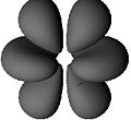
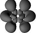
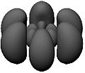
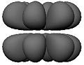
None of these images depicts an atom as it is. This is because it is impossible to even visualize an atom as it is. Whereas the best you can do with the images in the first row is to erase them from your memory—they represent a way of viewing the atom that is too simplified for the way we want to start thinking about it—the eight fuzzy images in the next row deserve scrutiny. Each represents an aspect of a stationary state of atomic hydrogen. You see neither the nucleus (a proton) nor the electron. What you see is a fuzzy position. To be precise, what you see are cloud-like blurs, which are symmetrical about the vertical and horizontal axes, and which represent the atom's internal relative position—the position of the electron relative to the proton or the position of the proton relative to the electron.

• What is the state of an atom?
• What is a stationary state?
• What exactly is a fuzzy position?
• How does such a blur represent the atom's internal relative position?
• Why can we not describe the atom's internal relative position as it is?

Quantum states

In quantum mechanics, states are probability algorithms. We use them to calculate the probabilities of the possible outcomes of measurements on the basis of actual measurement outcomes. A quantum state takes as its input

• one or several measurement outcomes,
• a measurement M,
• the time of M,

and it yields as its output the probabilities of the possible outcomes of M.

A quantum state is called stationary if the probabilities it assigns are independent of the time of the measurement.

From the mathematical point of view, each blur represents a density function $\rho ({\boldsymbol {r}})$. Imagine a small region $R$ like the little box inside the first blur. And suppose that this is a region of the (mathematical) space of positions relative to the proton. If you integrate $\rho ({\boldsymbol {r}})$ over $R,$ you obtain the probability $p\,(R)$ of finding the electron in $R,$ provided that the appropriate measurement is made:

$p\,(R)=\int _{R}\rho ({\boldsymbol {r}})\,d^{3}{\boldsymbol {r}}.$

"Appropriate" here means capable of ascertaining the truth value of the proposition "the electron is in $R$", the possible truth values being "true" or "false". What we see in each of the following images is a surface of constant probability density.

• 
  $\rho _{2p0}$
• 
  $\rho _{3p0}$
• 
  $\rho _{3d0}$
• 
  $\rho _{4p0}$
• 
  $\rho _{4d0}$
• 
  $\rho _{4f0}$
• 
  $\rho _{5d0}$
• 
  $\rho _{5f0}$

Now imagine that the appropriate measurement is made. Before the measurement, the electron is neither inside $R$ nor outside $R$. If it were inside, the probability of finding it outside would be zero, and if it were outside, the probability of finding it inside would be zero. After the measurement, on the other hand, the electron is either inside or outside $R.$

Conclusions:

• Before the measurement, the proposition "the electron is in $R$" is neither true nor false; it lacks a (definite) truth value.
• A measurement generally changes the state of the system on which it is performed.

As mentioned before, probabilities are assigned not only to measurement outcomes but also on the basis of measurement outcomes. Each density function $\rho _{nlm}$ serves to assign probabilities to the possible outcomes of a measurement of the electron's position relative to the proton. And in each case the assignment is based on the outcomes of a simultaneous measurement of three observables: the atom's energy (specified by the value of the principal quantum number $n$), its total angular momentum $l$ (specified by a letter, here p, d, or f), and the vertical component of its angular momentum $m$.

Fuzzy observables

We say that an observable $Q$ with a finite or countable number of possible values $q_{k}$ is fuzzy (or that it has a fuzzy value) if and only if at least one of the propositions "The value of $Q$ is $q_{k}$" lacks a truth value. This is equivalent to the following necessary and sufficient condition: the probability assigned to at least one of the values $q_{k}$ is neither 0 nor 1.

What about observables that are generally described as continuous, like a position?

The description of an observable as "continuous" is potentially misleading. For one thing, we cannot separate an observable and its possible values from a measurement and its possible outcomes, and a measurement with an uncountable set of possible outcomes is not even in principle possible. For another, there is not a single observable called "position". Different partitions of space define different position measurements with different sets of possible outcomes.

• Corollary: The possible outcomes of a position measurement (or the possible values of a position observable) are defined by a partition of space. They make up a finite or countable set of regions of space. An exact position is therefore neither a possible measurement outcome nor a possible value of a position observable.

So how do those cloud-like blurs represent the electron's fuzzy position relative to the proton? Strictly speaking, they graphically represent probability densities in the mathematical space of exact relative positions, rather than fuzzy positions. It is these probability densities that represent fuzzy positions by allowing us to calculate the probability of every possible value of every position observable.

It should now be clear why we cannot describe the atom's internal relative position as it is. To describe a fuzzy observable is to assign probabilities to the possible outcomes of a measurement. But a description that rests on the assumption that a measurement is made, does not describe an observable as it is (by itself, regardless of measurements).

Planck

Quantum mechanics began as a desperate measure to get around some spectacular failures of what subsequently came to be known as classical physics.

In 1900 Max Planck discovered a law that perfectly describes the spectrum of a glowing hot object. Planck's radiation formula turned out to be irreconcilable with the physics of his time. (If classical physics were right, you would be blinded by ultraviolet light if you looked at the burner of a stove, aka the UV catastrophe.) At first, it was just a fit to the data, "a fortuitous guess at an interpolation formula" as Planck himself called it. Only weeks later did it turn out to imply the quantization of energy for the emission of electromagnetic radiation: the energy $~E~$ of a quantum of radiation is proportional to the frequency $\nu$ of the radiation, the constant of proportionality being Planck's constant $~h~$

$~E=h\nu ~$.

We can of course use the angular frequency $~\omega =2\pi \nu ~$ instead of $\nu$. Introducing the reduced Planck constant $~\hbar =h/2\pi ~$, we then have

$E=\hbar \omega$.

This theory is valid at all temperatures and helpful in explaining radiation by black bodies.

Rutherford

In 1911 Ernest Rutherford proposed a model of the atom based on experiments by Geiger and Marsden. Geiger and Marsden had directed a beam of alpha particles at a thin gold foil. Most of the particles passed the foil more or less as expected, but about one in 8000 bounced back as if it had encountered a much heavier object. In Rutherford's own words this was as incredible as if you fired a 15 inch cannon ball at a piece of tissue paper and it came back and hit you. After analysing the data collected by Geiger and Marsden, Rutherford concluded that the diameter of the atomic nucleus (which contains over 99.9% of the atom's mass) was less than 0.01% of the diameter of the entire atom. He suggested that the atom is spherical in shape and the atomic electrons orbit the nucleus much like planets orbit a star. He calculated mass of electron as 1/7000th part of the mass of an alpha particle. Rutherford's atomic model is also called the Nuclear model.

The problem of having electrons orbit the nucleus the same way that a planet orbits a star is that classical electromagnetic theory demands that an orbiting electron will radiate away its energy and spiral into the nucleus in about 0.5×10^-10 seconds. This was the worst quantitative failure in the history of physics, under-predicting the lifetime of hydrogen by at least forty orders of magnitude! (This figure is based on the experimentally established lower bound on the proton's lifetime.)

Bohr

In 1913 Niels Bohr postulated that the angular momentum $L$ of an orbiting atomic electron was quantized: its "allowed" values are integral multiples of $\hbar$:

$L=n\hbar$ where $n=1,2,3,\dots$

Why quantize angular momentum, rather than any other quantity?

• Radiation energy of a given frequency is quantized in multiples of Planck's constant.
• Planck's constant is measured in the same units as angular momentum.

Bohr's postulate explained not only the stability of atoms but also why the emission and absorption of electromagnetic radiation by atoms is discrete. In addition it enabled him to calculate with remarkable accuracy the spectrum of atomic hydrogen — the frequencies at which it is able to emit and absorb light (visible as well as infrared and ultraviolet). The following image shows the visible emission spectrum of atomic hydrogen, which contains four lines of the Balmer series.

Visible emission spectrum of atomic hydrogen, containing four lines of the Balmer series.

Apart from his quantization postulate, Bohr's reasoning at this point remained completely classical. Let's assume with Bohr that the electron's orbit is a circle of radius $r.$ The speed of the electron is then given by $v=r\,d\beta /dt,$ and the magnitude of its acceleration by $a=dv/dt=v\,d\beta /dt.$ Eliminating $d\beta /dt$ yields $a=v^{2}/r.$ In the cgs system of units, the magnitude of the Coulomb force is simply $F=e^{2}/r^{2},$ where $e$ is the magnitude of the charge of both the electron and the proton. Via Newton's $F=ma$ the last two equations yield $m_{e}v^{2}=e^{2}/r,$ where $m_{e}$ is the electron's mass. If we take the proton to be at rest, we obtain $T=m_{e}v^{2}/2=e^{2}/2r$ for the electron's kinetic energy.

If the electron's potential energy at infinity is set to 0, then its potential energy $V$ at a distance $r$ from the proton is minus the work required to move it from $r$ to infinity,

$V=-\int _{r}^{\infty }F(r')\,dr'=-\int _{r}^{\infty }\!{e^{2} \over (r')^{2}}\,dr'=+\left[{e^{2} \over r'}\right]_{r}^{\infty }=0-{e^{2} \over r}.$

The total energy of the electron thus is

$E=T+V=e^{2}/2r-e^{2}/r=-e^{2}/2r.$

We want to express this in terms of the electron's angular momentum $L=m_{e}vr.$ Remembering that $m_{e}v^{2}=e^{2}/r,$ and hence $rm_{e}^{2}v^{2}=m_{e}e^{2},$ and multiplying the numerator $e^{2}\,$ by $m_{e}e^{2}$ and the denominator $2r$ by $rm_{e}^{2}v^{2},$ we obtain

$E=-{e^{2} \over 2r}=-{m_{e}e^{4} \over 2m_{e}^{2}v^{2}r^{2}}=-{m_{e}e^{4} \over 2L^{2}}.$

Now comes Bohr's break with classical physics: he simply replaced $L$ by $n\hbar$. The "allowed" values for the angular momentum define a series of allowed values for the atom's energy:

$E_{n}=-{1 \over n^{2}}\left({m_{e}e^{4} \over 2\hbar ^{2}}\right),\quad n=1,2,3,\dots$

As a result, the atom can emit or absorb energy only by amounts equal to the absolute values of the differences

$\Delta E_{nm}=E_{n}-E_{m}=\left({1 \over n^{2}}-{1 \over m^{2}}\right)\,{\hbox{Ry}},$

one Rydberg (Ry) being equal to $m_{e}e^{4}/2\hbar ^{2}=13.6056923(12)\,{\hbox{eV.}}$ This is also the ionization energy $\Delta E_{1\infty }$ of atomic hydrogen — the energy needed to completely remove the electron from the proton. Bohr's predicted value was found to be in excellent agreement with the measured value.

Using two of the above expressions for the atom's energy and solving for $r,$ we obtain $r=n^{2}\hbar ^{2}/m_{e}e^{2}.$ For the ground state $(n=1)$ this is the Bohr radius of the hydrogen atom, which equals $\hbar ^{2}/m_{e}e^{2}=5.291772108(18)\times 10^{-11}m.$ The mature theory yields the same figure but interprets it as the most likely distance from the proton at which the electron would be found if its distance from the proton were measured.

de Broglie

In 1923, ten years after Bohr had derived the spectrum of atomic hydrogen by postulating the quantization of angular momentum, Louis de Broglie hit on an explanation of why the atom's angular momentum comes in multiples of $\hbar .$ Since 1905, Einstein had argued that electromagnetic radiation itself was quantized (and not merely its emission and absorption, as Planck held). If electromagnetic waves can behave like particles (now known as photons), de Broglie reasoned, why cannot electrons behave like waves?

Suppose that the electron in a hydrogen atom is a standing wave on what has so far been thought of as the electron's circular orbit. (The crests, troughs, and nodes of a standing wave are stationary.) For such a wave to exist on a circle, the circumference of the latter must be an integral multiple of the wavelength $\lambda$ of the former: $2\pi r=n\lambda .$

• 
• 
• 
• 

Einstein had established not only that electromagnetic radiation of frequency $\nu$ comes in quanta of energy $E=h\nu$ but also that these quanta carry a momentum $p=h/\lambda .$ Using this formula to eliminate $\lambda$ from the condition $2\pi r=n\lambda ,$ one obtains $pr=n\hbar .$ But $pr=mvr$ is just the angular momentum $L$ of a classical electron with an orbit of radius $r.$ In this way de Broglie derived the condition $L=n\hbar$ that Bohr had simply postulated.

Schrödinger

If the electron is a standing wave, why should it be confined to a circle? After de Broglie's crucial insight that particles are waves of some sort, it took less than three years for the mature quantum theory to be found, not once, but twice. By Werner Heisenberg in 1925 and by Erwin Schrödinger in 1926. If we let the electron be a standing wave in three dimensions, we have all it takes to arrive at the Schrödinger equation, which is at the heart of the mature theory.

Let's keep to one spatial dimension. The simplest mathematical description of a wave of angular wavenumber $k=2\pi /\lambda$ and angular frequency $\omega =2\pi /T=2\pi \nu$ (at any rate, if you are familiar with complex numbers) is the function

$\psi (x,t)=e^{i(kx-\omega t)}.$

Let's express the phase $\phi (x,t)=kx-\omega t$ in terms of the electron's energy $E=h\nu =\hbar \omega$ and momentum $p=h/\lambda =\hbar k:$

$\psi (x,t)=e^{i(px-Et)/\hbar }.$

The partial derivatives with respect to $x$ and $t$ are

${\partial \psi \over \partial x}={i \over \hbar }p\psi \quad {\hbox{and}}\quad {\partial \psi \over \partial t}=-{i \over \hbar }E\psi .$

We also need the second partial derivative of $\psi$ with respect to $x$:

${\partial ^{2}\psi \over \partial x^{2}}=\left({ip \over \hbar }\right)^{2}\psi .$

We thus have

$E\psi =i\hbar {\partial \psi \over \partial t},\quad p\psi =-i\hbar {\partial \psi \over \partial x},\quad {\hbox{and}}\quad p^{2}\psi =-\hbar ^{2}{\partial ^{2}\psi \over \partial x^{2}}.$

In non-relativistic classical physics the kinetic energy and the kinetic momentum $p$ of a free particle are related via the dispersion relation

$E=p^{2}/2m.$

This relation also holds in non-relativistic quantum physics. Later you will learn why.

In three spatial dimensions, $p$ is the magnitude of a vector ${\textbf {p}}$. If the particle also has a potential energy $V({\textbf {r}},t)$ and a potential momentum ${\textbf {A}}({\textbf {r}},t)$ (in which case it is not free), and if $E$ and ${\textbf {p}}$ stand for the particle's total energy and total momentum, respectively, then the dispersion relation is

$E-V=({\textbf {p}}-{\textbf {A}})^{2}/2m.$

By the square of a vector ${\textbf {v}}$ we mean the dot (or scalar) product ${\textbf {v}}\cdot {\textbf {v}}$. Later you will learn why we represent possible influences on the motion of a particle by such fields as $V({\textbf {r}},t)$ and ${\textbf {A}}({\textbf {r}},t).$

Returning to our fictitious world with only one spatial dimension, allowing for a potential energy $V(x,t)$, substituting the differential operators $i\hbar {\partial \over \partial t}$ and $-\hbar ^{2}{\partial ^{2} \over \partial x^{2}}$ for $E$ and $p^{2}$ in the resulting dispersion relation, and applying both sides of the resulting operator equation to $\psi ,$ we arrive at the one-dimensional (time-dependent) Schrödinger equation:

$i\hbar {\partial \psi \over \partial t}=-{\hbar ^{2} \over 2m}{\partial ^{2}\psi \over \partial x^{2}}+V\psi$

In three spatial dimensions and with both potential energy $V({\textbf {r}},t)$ and potential momentum ${\textbf {A}}({\textbf {r}},t)$ present, we proceed from the relation $E-V=({\textbf {p}}-{\textbf {A}})^{2}/2m,$ substituting $i\hbar {\partial \over \partial t}$ for $E$ and $-i\hbar {\partial \over \partial {\textbf {r}}}$ for ${\textbf {p}}.$ The differential operator ${\partial \over \partial {\textbf {r}}}$ is a vector whose components are the differential operators $\left({\partial \psi \over \partial x},{\partial \psi \over \partial y},{\partial \psi \over \partial z}\right).$ The result:

$i\hbar {\partial \psi \over \partial t}={\frac {1}{2m}}\left(-i\hbar {\partial \over \partial {\textbf {r}}}-{\textbf {A}}\right)^{2}\psi +V\psi ,$

where $\psi$ is now a function of ${\textbf {r}}=(x,y,z)$ and $t.$ This is the three-dimensional Schrödinger equation. In non-relativistic investigations (to which the Schrödinger equation is confined) the potential momentum can generally be ignored, which is why the Schrödinger equation is often given this form:

$i\hbar {\partial \psi \over \partial t}=-{\hbar ^{2} \over 2m}\left({\partial ^{2}\psi \over \partial x^{2}}+{\partial ^{2}\psi \over \partial y^{2}}+{\partial ^{2}\psi \over \partial z^{2}}\right)+V\psi$

The free Schrödinger equation (without even the potential energy term) is satisfied by $\psi (x,t)=e^{i(kx-\omega t)}$ (in one dimension) or $\psi ({\textbf {r}},t)=e^{i(\mathbf {k} \cdot \mathbf {r} -\omega t)}$ (in three dimensions) provided that $E=\hbar {\omega }$ equals $p^{2}/2m=(\hbar k)^{2}/2m,$ which is to say: $\omega (k)=\hbar k^{2}/2m.$ However, since we are dealing with a homogeneous linear differential equation — which tells us that solutions may be added and/or multiplied by an arbitrary constant to yield additional solutions — any function of the form

$\psi (x,t)={1 \over {\sqrt {2\pi }}}\int {\overline {\psi }}(k)\,e^{i[kx-\omega (k)t]}dk={1 \over {\sqrt {2\pi }}}\int {\overline {\psi }}(k,t)\,e^{ikx}dk$

with ${\overline {\psi }}(k,t)={\overline {\psi }}(k)e^{-i\omega (k)t}$ solves the (one-dimensional) Schrödinger equation. If no integration boundaries are specified, then we integrate over the real line, i.e., the integral is defined as the limit $\lim _{L\rightarrow \infty }\int _{-L}^{+L}.$ The converse also holds: every solution is of this form. The factor in front of the integral is present for purely cosmetic reasons, as you will realize presently. ${\overline {\psi }}(k,t)$ is the Fourier transform of $\psi (x,t),$ which means that

${\overline {\psi }}(k,t)={1 \over {\sqrt {2\pi }}}\int \psi (x,t)\,e^{-ikx}dx.$

The Fourier transform of $\psi (x,t)$ exists because the integral $\int |\psi (x,t)|dx$ is finite. In the next section we will come to know the physical reason why this integral is finite.

So now we have a condition that every electron "wave function" must satisfy in order to satisfy the appropriate dispersion relation. If this (and hence the Schrödinger equation) contains either or both of the potentials ${\textbf {V}}$ and ${\textbf {A}}$, then finding solutions can be tough. As a budding quantum mechanician, you will spend a considerable amount of time learning to solve the Schrödinger equation with various potentials.

Born

In the same year that Erwin Schrödinger published the equation that now bears his name, the nonrelativistic theory was completed by Max Born's insight that the Schrödinger wave function $\psi (\mathbf {r} ,t)$ is actually nothing but a tool for calculating probabilities, and that the probability of detecting a particle "described by" $\psi (\mathbf {r} ,t)$ in a region of space $R$ is given by the volume integral

$\int _{R}|\psi (t,\mathbf {r} )|^{2}\,d^{3}r=\int _{R}\psi ^{*}\psi \,d^{3}r$

— provided that the appropriate measurement is made, in this case a test for the particle's presence in $R$. Since the probability of finding the particle somewhere (no matter where) has to be 1, only a square integrable function can "describe" a particle. This rules out $\psi (\mathbf {r} )=e^{i\mathbf {k} \cdot \mathbf {r} },$ which is not square integrable. In other words, no particle can have a momentum so sharp as to be given by $\hbar$ times a wave vector $\mathbf {k}$, rather than by a genuine probability distribution over different momenta.

Given a probability density function $|\psi (x)|^{2}$, we can define the expected value

$\langle x\rangle =\int |\psi (x)|^{2}\,x\,dx=\int \psi ^{*}\,x\,\psi \,dx$

and the standard deviation  $\Delta x={\sqrt {\int |\psi |^{2}(x-\langle x\rangle )^{2}}}$

as well as higher moments of $|\psi (x)|^{2}$. By the same token,

$\langle k\rangle =\int {\overline {\psi }}\,^{*}\,k\,{\overline {\psi }}\,dk$  and  $\Delta k={\sqrt {\int |{\overline {\psi }}|^{2}(k-\langle k\rangle )^{2}}}.$

Here is another expression for $\langle k\rangle :$

$\langle k\rangle =\int \psi ^{*}(x)\left(-i{\frac {d}{dx}}\right)\psi (x)\,dx.$

To check that the two expressions are in fact equal, we plug  $\psi (x)=(2\pi )^{-1/2}\int {\overline {\psi }}(k)\,e^{ikx}dk$  into the latter expression:

$\langle k\rangle ={\frac {1}{\sqrt {2\pi }}}\int \psi ^{*}(x)\left(-i{\frac {d}{dx}}\right)\int {\overline {\psi }}(k)\,e^{ikx}dk\,dx={\frac {1}{\sqrt {2\pi }}}\int \psi ^{*}(x)\int {\overline {\psi }}(k)\,k\,e^{ikx}dk\,dx.$

Next we replace $\psi ^{*}(x)$ by $(2\pi )^{-1/2}\int {\overline {\psi }}\,^{*}(k')\,e^{-ik'x}dk'$  and shuffle the integrals with the mathematical nonchalance that is common in physics:

$\langle k\rangle =\int \!\int {\overline {\psi }}\,^{*}(k')\,k\,{\overline {\psi }}(k)\left[{\frac {1}{2\pi }}\int e^{i(k-k')x}dx\right]dk\,dk'.$

The expression in square brackets is a representation of Dirac's delta distribution $\delta (k-k'),$ the defining characteristic of which is  $\int _{-\infty }^{+\infty }f(x)\,\delta (x)\,dx=f(0)$  for any continuous function $f(x).$ (In case you didn't notice, this proves what was to be proved.)

Heisenberg

In the same annus mirabilis of quantum mechanics, 1926, Werner Heisenberg proved the so-called "uncertainty" relation

$\Delta x\,\Delta p\geq \hbar /2.$

Heisenberg spoke of Unschärfe, the literal translation of which is "fuzziness" rather than "uncertainty". Since the relation $\Delta x\,\Delta k\geq 1/2$ is a consequence of the fact that $\psi (x)$ and ${\overline {\psi }}(k)$ are related to each other via a Fourier transformation, we leave the proof to the mathematicians. The fuzziness relation for position and momentum follows via $p=\hbar k$. It says that the fuzziness of a position (as measured by $\Delta x$ ) and the fuzziness of the corresponding momentum (as measured by $\Delta p=\hbar \Delta k$ ) must be such that their product equals at least $\hbar /2.$

The Feynman route to Schrödinger

The probabilities of the possible outcomes of measurements performed at a time $t_{2}$ are determined by the Schrödinger wave function $\psi (\mathbf {r} ,t_{2})$. The wave function $\psi (\mathbf {r} ,t_{2})$ is determined via the Schrödinger equation by $\psi (\mathbf {r} ,t_{1}).$ What determines $\psi (\mathbf {r} ,t_{1})$ ? Why, the outcome of a measurement performed at $t_{1}$ — what else? Actual measurement outcomes determine the probabilities of possible measurement outcomes.

Two rules

In this chapter we develop the quantum-mechanical probability algorithm from two fundamental rules. To begin with, two definitions:

• Alternatives are possible sequences of measurement outcomes.
• With each alternative is associated a complex number called amplitude.

Suppose that you want to calculate the probability of a possible outcome of a measurement given the actual outcome of an earlier measurement. Here is what you have to do:

• Choose any sequence of measurements that may be made in the meantime.
• Assign an amplitude to each alternative.
• Apply either of the following rules:

Rule A: If the intermediate measurements are made (or if it is possible to infer from other measurements what their outcomes would have been if they had been made), first square the absolute values of the amplitudes of the alternatives and then add the results.

Rule B: If the intermediate measurements are not made (and if it is not possible to infer from other measurements what their outcomes would have been), first add the amplitudes of the alternatives and then square the absolute value of the result.

In subsequent sections we will explore the consequences of these rules for a variety of setups, and we will think about their origin — their raison d'être. Here we shall use Rule B to determine the interpretation of ${\overline {\psi }}(k)$ given Born's probabilistic interpretation of $\psi (x)$.

In the so-called "continuum normalization", the unphysical limit of a particle with a sharp momentum $\hbar k'$ is associated with the wave function

$\psi _{k'}(x,t)={\frac {1}{\sqrt {2\pi }}}\int \delta (k-k')\,e^{i[kx-\omega (k)t]}dk={\frac {1}{\sqrt {2\pi }}}\,e^{i[k'x-\omega (k')t]}.$

Hence we may write $\psi (x,t)=\int {\overline {\psi }}(k)\,\psi _{k}(x,t)\,dk.$

${\overline {\psi }}(k)$ is the amplitude for the outcome $\hbar k$ of an infinitely precise momentum measurement. $\psi _{k}(x,t)$ is the amplitude for the outcome $x$ of an infinitely precise position measurement performed (at time t) subsequent to an infinitely precise momentum measurement with outcome $\hbar k.$ And $\psi (x,t)$ is the amplitude for obtaining $x$ by an infinitely precise position measurement performed at time $t.$

The preceding equation therefore tells us that the amplitude for finding $x$ at $t$ is the product of

1. the amplitude for the outcome $\hbar k$ and
2. the amplitude for the outcome $x$ (at time $t$) subsequent to a momentum measurement with outcome $\hbar k,$

summed over all values of $k.$

Under the conditions stipulated by Rule A, we would have instead that the probability for finding $x$ at $t$ is the product of

1. the probability for the outcome $\hbar k$ and
2. the probability for the outcome $x$ (at time $t$) subsequent to a momentum measurement with outcome $\hbar k,$

summed over all values of $k.$

The latter is what we expect on the basis of standard probability theory. But if this holds under the conditions stipulated by Rule A, then the same holds with "amplitude" substituted from "probability" under the conditions stipulated by Rule B. Hence, given that $\psi _{k}(x,t)$ and $\psi (x,t)$ are amplitudes for obtaining the outcome $x$ in an infinitely precise position measurement, ${\overline {\psi }}(k)$ is the amplitude for obtaining the outcome $\hbar k$ in an infinitely precise momentum measurement.

Notes:

1. Since Rule B stipulates that the momentum measurement is not actually made, we need not worry about the impossibility of making an infinitely precise momentum measurement.
2. If we refer to $|\psi (x)|^{2}$ as "the probability of obtaining the outcome $x,$" what we mean is that $|\psi (x)|^{2}$ integrated over any interval or subset of the real line is the probability of finding our particle in this interval or subset.

An experiment with two slits

The setup

In this experiment, the final measurement (to the possible outcomes of which probabilities are assigned) is the detection of an electron at the backdrop, by a detector situated at D (D being a particular value of x). The initial measurement outcome, on the basis of which probabilities are assigned, is the launch of an electron by an electron gun G. (Since we assume that G is the only source of free electrons, the detection of an electron behind the slit plate also indicates the launch of an electron in front of the slit plate.) The alternatives or possible intermediate outcomes are

• the electron went through the left slit (L),
• the electron went through the right slit (R).

The corresponding amplitudes are $A_{L}$ and $A_{R}.$

Here is what we need to know in order to calculate them:

• $A_{L}$ is the product of two complex numbers, for which we shall use the symbols $\langle D|L\rangle$ and $\langle L|G\rangle .$
• By the same token, $A_{R}=\langle D|R\rangle \,\langle R|G\rangle .$
• The absolute value of $\langle B|A\rangle$ is inverse proportional to the distance $d(BA)$ between A and B.
• The phase of $\langle B|A\rangle$ is proportional to $d(BA).$

For obvious reasons $\langle B|A\rangle$ is known as a propagator.

Why product?

Recall the fuzziness ("uncertainty") relation, which implies that $\Delta p\rightarrow \infty$ as $\Delta x\rightarrow 0.$ In this limit the particle's momentum is completely indefinite or, what comes to the same, has no value at all. As a consequence, the probability of finding a particle at B, given that it was last "seen" at A, depends on the initial position A but not on any initial momentum, inasmuch as there is none. Hence whatever the particle does after its detection at A is independent of what it did before then. In probability-theoretic terms this means that the particle's propagation from G to L and its propagation from L to D are independent events. So the probability of propagation from G to D via L is the product of the corresponding probabilities, and so the amplitude of propagation from G to D via L is the product $\langle D|L\,\rangle \langle L|G\rangle$ of the corresponding amplitudes.

Why is the absolute value inverse proportional to the distance?

Imagine (i) a sphere of radius $r$ whose center is A and (ii) a detector monitoring a unit area of the surface of this sphere. Since the total surface area is proportional to $r^{2},$ and since for a free particle the probability of detection per unit area is constant over the entire surface (explain why!), the probability of detection per unit area is inverse proportional to $r^{2}.$ The absolute value of the amplitude of detection per unit area, being the square root of the probability, is therefore inverse proportional to $r.$

Why is the phase proportional to the distance?

The multiplicativity of successive propagators implies the additivity of their phases. Together with the fact that, in the case of a free particle, the propagator $\langle B|A\rangle$ (and hence its phase) can only depend on the distance between A and B, it implies the proportionality of the phase of $\langle B|A\rangle$ to $d(BA).$

Calculating the interference pattern

According to Rule A, the probability of detecting at G an electron launched at D is

$p_{A}(D)=|\langle D|L\rangle \,\langle L|G\rangle |^{2}+|\langle D|R\rangle \,\langle R|G\rangle |^{2}.$

If the slits are equidistant from G, then $\langle L|G\rangle$ and $\langle R|G\rangle$ are equal and $p_{A}(D)$ is proportional to

$|\langle D|L\rangle |^{2}+|\langle D|R\rangle |^{2}=1/d^{2}(DL)+1/d^{2}(DR).$

Here is the resulting plot of $p_{A}$ against the position $x$ of the detector:

Predicted relative frequency of detection according to Rule A

$p_{A}(x)$ (solid line) is the sum of two distributions (dotted lines), one for the electrons that went through L and one for the electrons that went through R.

According to Rule B, the probability $p_{B}(D)$ of detecting at D an electron launched at G is proportional to

$|\langle D|L\rangle +\langle D|R\rangle |^{2}=1/d^{2}(DL)+1/d^{2}(DR)+2\cos(k\Delta )/[d(DL)\,d(DR)],$

where $\Delta$ is the difference $d(DR)-d(DL)$ and $k=p/\hbar$ is the wavenumber, which is sufficiently sharp to be approximated by a number. (And it goes without saying that you should check this result.)

Here is the plot of $p_{B}$ against $x$ for a particular set of values for the wavenumber, the distance between the slits, and the distance between the slit plate and the backdrop:

Predicted relative frequency of detection according to Rule B

Observe that near the minima the probability of detection is less if both slits are open than it is if one slit is shut. It is customary to say that destructive interference occurs at the minima and that constructive interference occurs at the maxima, but do not think of this as the description of a physical process. All we mean by "constructive interference" is that a probability calculated according to Rule B is greater than the same probability calculated according to Rule A, and all we mean by "destructive interference" is that a probability calculated according to Rule B is less than the same probability calculated according to Rule A.

Here is how an interference pattern builds up over time:

• 
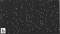  100 electrons
• 
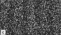  3000 electrons
• 
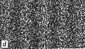  20000 electrons
• 
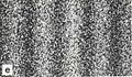  70000 electrons

Bohm's story

Hidden Variables

Suppose that the conditions stipulated by Rule B are met: there is nothing — no event, no state of affairs, anywhere, anytime — from which the slit taken by an electron can be inferred. Can it be true, in this case,

• that each electron goes through a single slit — either L or R — and
• that the behavior of an electron that goes through one slit does not depend on whether the other slit is open or shut?

To keep the language simple, we will say that an electron leaves a mark where it is detected at the backdrop. If each electron goes through a single slit, then the observed distribution of marks when both slits are open is the sum of two distributions, one from electrons that went through L and one from electrons that went through R:

$p_{B}(x)=p_{L}(x)+p_{R}(x)\,\!$

If in addition the behavior of an electron that goes through one slit does not depend on whether the other slit is open or shut, then we can observe $p_{L}(x)$ by keeping R shut, and we can observe $p_{R}(x)$ by keeping L shut. What we observe if R is shut is the left dashed hump, and what we observed if L is shut is the right dashed hump:

Hence if the above two conditions (as well as those stipulated by Rule B) are satisfied, we will see the sum of these two humps. In reality what we see is this:

Thus all of those conditions cannot be simultaneously satisfied. If Rule B applies, then either it is false that each electron goes through a single slit or the behavior of an electron that goes through one slit does depend on whether the other slit is open or shut.

Which is it?

According to one attempt to make physical sense of the mathematical formalism of quantum mechanics, due to Louis de Broglie and David Bohm, each electron goes through a single slit, and the behavior of an electron that goes through one slit depends on whether the other slit is open or shut.

So how does the state of, say, the right slit (open or shut) affect the behavior of an electron that goes through the left slit? In both de Broglie's pilot wave theory and Bohmian mechanics, the electron is assumed to be a well-behaved particle in the sense that it follows a precise path — its position at any moment is given by three coordinates — and in addition there exists a wave that guides the electron by exerting on it a force. If only one slit is open, this passes through one slit. If both slits are open, this passes through both slits and interferes with itself (in the "classical" sense of interference). As a result, it guides the electrons along wiggly paths that cluster at the backdrop so as to produce the observed interference pattern:

According to this story, the reason why electrons coming from the same source or slit arrive in different places, is that they start out in slightly different directions and/or with slightly different speeds. If we had exact knowledge of their initial positions and momenta, we could make an exact prediction of each electron's subsequent motion. Obtaining this exact knowledge, however, is impossible in practice. The [[../../Serious illnesses/Born#Heisenberg|uncertainty principle ]] prevents us from making exact predictions of a particle's motion. Hence even though according to Bohm the initial positions and momenta are in possession of precise values, we can never know them.

If positions and momenta have precise values, then why can we not measure them? It used to be said that this is because a measurement exerts an uncontrollable influence on the value of the observable being measured. Yet this merely raises another question: why do measurements exert uncontrollable influences? This may be true for all practical purposes, but the uncertainty principle does not say that $\Delta x\,\Delta p\geq \hbar /2$ merely holds for all practical purposes. Moreover, it isn't the case that measurements necessarily "disturb" the systems on which they are performed.

The statistical element of quantum mechanics is an essential feature of the theory. The postulate of an underlying determinism, which in order to be consistent with the theory has to be a crypto-determinism, not only adds nothing to our understanding of the theory but also precludes any proper understanding of this essential feature of the theory. There is, in fact, a simple and obvious reason why hidden variables are hidden: the reason why they are strictly (rather than merely for all practical purposes) unobservable is that they do not exist.

At one time Einstein insisted that theories ought to be formulated without reference to unobservable quantities. When Heisenberg later mentioned to Einstein that this maxim had guided him in his discovery of the uncertainty principle, Einstein replied something to this effect: "Even if I once said so, it is nonsense." His point was that before one has a theory, one cannot know what is observable and what is not. Our situation here is different. We have a theory, and this tells in no uncertain terms what is observable and what is not.

Propagator for a free and stable particle

The propagator as a path integral

Suppose that we make m intermediate position measurements at fixed intervals of duration $\Delta t.$ Each of these measurements is made with the help of an array of detectors monitoring n mutually disjoint regions $R_{k},$ $k=1,\dots ,n.$ Under the conditions stipulated by Rule B, the propagator $\langle B|A\rangle$ now equals the sum of amplitudes

$\sum _{k_{1}=1}^{n}\cdots \sum _{k_{m}=1}^{n}\langle B|R_{k_{m}}\rangle \cdots \langle R_{k_{2}}|R_{k_{1}}\rangle \,\langle R_{k_{1}}|A\rangle .$

It is not hard to see what happens in the double limit $\Delta t\rightarrow 0$ (which implies that $m\rightarrow \infty$) and $n\rightarrow \infty .$ The multiple sum $\sum _{k_{1}=1}^{n}\cdots \sum _{k_{m}=1}^{n}$ becomes an integral $\int \!{\mathcal {DC}}$ over continuous spacetime paths from A to B, and the amplitude $\langle B|R_{k_{m}}\rangle \cdots \langle R_{k_{1}}|A\rangle$ becomes a complex-valued functional $Z[{\mathcal {C}}:A\rightarrow B]$ — a complex function of continuous functions representing continuous spacetime paths from A to B:

$\langle B|A\rangle =\int \!{\mathcal {DC}}\,Z[{\mathcal {C}}:A\rightarrow B]$

The integral $\int \!{\mathcal {DC}}$ is not your standard Riemann integral $\int _{a}^{b}dx\,f(x),$ to which each infinitesimal interval $dx$ makes a contribution proportional to the value that $f(x)$ takes inside the interval, but a functional or path integral, to which each "bundle" of paths of infinitesimal width ${\mathcal {DC}}$ makes a contribution proportional to the value that $Z[{\mathcal {C}}]$ takes inside the bundle.

As it stands, the path integral $\int \!{\mathcal {DC}}$ is just the idea of an idea. Appropriate evaluation methods have to be devised on a more or less case-by-case basis.

A free particle

Now pick any path ${\mathcal {C}}$ from A to B, and then pick any infinitesimal segment $d{\mathcal {C}}$ of ${\mathcal {C}}$. Label the start and end points of $d{\mathcal {C}}$ by inertial coordinates $t,x,y,z$ and $t+dt,x+dx,y+dy,z+dz,$ respectively. In the general case, the amplitude $Z(d{\mathcal {C}})$ will be a function of $t,x,y,z$ and $dt,dx,dy,dz.$ In the case of a free particle, $Z(d{\mathcal {C}})$ depends neither on the position of $d{\mathcal {C}}$ in spacetime (given by $t,x,y,z$) nor on the spacetime orientiaton of $d{\mathcal {C}}$ (given by the four-velocity $(c\,dt/ds,dx/ds,dy/ds,dz/ds)$ but only on the proper time interval $ds={\sqrt {dt^{2}-(dx^{2}+dy^{2}+dz^{2})/c^{2}}}.$

(Because its norm equals the speed of light, the four-velocity depends on three rather than four independent parameters. Together with $ds,$ they contain the same information as the four independent numbers $dt,dx,dy,dz.$)

Thus for a free particle $Z(d{\mathcal {C}})=Z(ds).$ With this, the multiplicativity of successive propagators tells us that

$\prod _{j}Z(ds_{j})=Z{\Bigl (}\sum _{j}ds_{j}{\Bigr )}\longrightarrow Z{\Bigl (}\int _{\mathcal {C}}ds{\Bigr )}$

It follows that there is a complex number $z$ such that $Z[{\mathcal {C}}]=e^{z\,s[{\mathcal {C}}:A\rightarrow B]},$ where the line integral $s[{\mathcal {C}}:A\rightarrow B]=\int _{\mathcal {C}}ds$ gives the time that passes on a clock as it travels from A to B via ${\mathcal {C}}.$

A free and stable particle

By integrating ${\bigl |}\langle B|A\rangle {\bigr |}^{2}$ (as a function of $\mathbf {r} _{B}$) over the whole of space, we obtain the probability of finding that a particle launched at the spacetime point $t_{A},\mathbf {r} _{A}$ still exists at the time $t_{B}.$ For a stable particle this probability equals 1:

$\int \!d^{3}r_{B}\left|\langle t_{B},\mathbf {r} _{B}|t_{A},\mathbf {r} _{A}\rangle \right|^{2}=\int \!d^{3}r_{B}\left|\int \!{\mathcal {DC}}\,e^{z\,s[{\mathcal {C}}:A\rightarrow B]}\right|^{2}=1$

If you contemplate this equation with a calm heart and an open mind, you will notice that if the complex number $z=a+ib$ had a real part $a\neq 0,$ then the integral between the two equal signs would either blow up $(a>0)$ or drop off $(a<0)$ exponentially as a function of $t_{B}$, due to the exponential factor $e^{a\,s[{\mathcal {C}}]}$.

Meaning of mass

The propagator for a free and stable particle thus has a single "degree of freedom": it depends solely on the value of $b.$ If proper time is measured in seconds, then $b$ is measured in radians per second. We may think of $e^{ib\,s},$ with $s$ a proper-time parametrization of ${\mathcal {C}},$ as a clock carried by a particle that travels from A to B via ${\mathcal {C}},$ provided we keep in mind that we are thinking of an aspect of the mathematical formalism of quantum mechanics rather than an aspect of the real world.

It is customary

• to insert a minus (so the clock actually turns clockwise!): $Z=e^{-ib\,s[{\mathcal {C}}]},$
• to multiply by $2\pi$ (so that we may think of $b$ as the rate at which the clock "ticks" — the number of cycles it completes each second): $Z=e^{-i\,2\pi \,b\,s[{\mathcal {C}}]},$
• to divide by Planck's constant $h$ (so that $b$ is measured in energy units and called the rest energy of the particle): $Z=e^{-i(2\pi /h)\,b\,s[{\mathcal {C}}]}=e^{-(i/\hbar )\,b\,s[{\mathcal {C}}]},$
• and to multiply by $c^{2}$ (so that $b$ is measured in mass units and called the particle's rest mass): $Z=e^{-(i/\hbar )\,b\,c^{2}\,s[{\mathcal {C}}]}.$

The purpose of using the same letter $b$ everywhere is to emphasize that it denotes the same physical quantity, merely measured in different units. If we use natural units in which $\hbar =c=1,$ rather than conventional ones, the identity of the various $b$'s is immediately obvious.

From quantum to classical

Action

Let's go back to the propagator

$\langle B|A\rangle =\int \!{\mathcal {DC}}\,Z[{\mathcal {C}}:A\rightarrow B].$

For a free and stable particle we found that

$Z[{\mathcal {C}}]=e^{-(i/\hbar )\,m\,c^{2}\,s[{\mathcal {C}}]},\qquad s[{\mathcal {C}}]=\int _{\mathcal {C}}ds,$

where $ds={\sqrt {dt^{2}-(dx^{2}+dy^{2}+dz^{2})/c^{2}}}$ is the proper-time interval associated with the path element $d{\mathcal {C}}$. For the general case we found that the amplitude $Z(d{\mathcal {C}})$ is a function of $t,x,y,z$ and $dt,dx,dy,dz$ or, equivalently, of the coordinates $t,x,y,z$, the components $c\,dt/ds,dx/ds,dy/ds,dz/ds$ of the 4-velocity, as well as $ds$. For a particle that is stable but not free, we obtain, by the same argument that led to the above amplitude,

$Z[{\mathcal {C}}]=e^{(i/\hbar )\,S[{\mathcal {C}}]},$

where we have introduced the functional $S[{\mathcal {C}}]=\int _{\mathcal {C}}dS$, which goes by the name action.

For a free and stable particle, $S[{\mathcal {C}}]$ is the proper time (or proper duration) $s[{\mathcal {C}}]=\int _{\mathcal {C}}ds$ multiplied by $-mc^{2}$, and the infinitesimal action $dS[d{\mathcal {C}}]$ is proportional to $ds$:

$S[{\mathcal {C}}]=-m\,c^{2}\,s[{\mathcal {C}}],\qquad dS[d{\mathcal {C}}]=-m\,c^{2}\,ds.$

Let's recap. We know all about the motion of a stable particle if we know how to calculate the probability $p(B|A)$ (in all circumstances). We know this if we know the amplitude $\langle B|A\rangle$. We know the latter if we know the functional $Z[{\mathcal {C}}]$. And we know this functional if we know the infinitesimal action $dS(t,x,y,z,dt,dx,dy,dz)$ or $dS(t,\mathbf {r} ,dt,d\mathbf {r} )$ (in all circumstances).

What do we know about $dS$?

The multiplicativity of successive propagators implies the additivity of actions associated with neighboring infinitesimal path segments $d{\mathcal {C}}_{1}$ and $d{\mathcal {C}}_{2}$. In other words,

$e^{(i/\hbar )\,dS(d{\mathcal {C}}_{1}+d{\mathcal {C}}_{2})}=e^{(i/\hbar )\,dS(d{\mathcal {C}}_{2})}\,e^{(i/\hbar )\,dS(d{\mathcal {C}}_{1})}$

implies

$dS(d{\mathcal {C}}_{1}+d{\mathcal {C}}_{2})=dS(d{\mathcal {C}}_{1})+dS(d{\mathcal {C}}_{2}).$

It follows that the differential $dS$ is homogeneous (of degree 1) in the differentials $dt,d\mathbf {r}$:

$dS(t,\mathbf {r} ,\lambda \,dt,\lambda \,d\mathbf {r} )=\lambda \,dS(t,\mathbf {r} ,dt,d\mathbf {r} ).$

This property of $dS$ makes it possible to think of the action $S[{\mathcal {C}}]$ as a (particle-specific) length associated with ${\mathcal {C}}$, and of $dS$ as defining a (particle-specific) spacetime geometry. By substituting $1/dt$ for $\lambda$ we get:

$dS(t,\mathbf {r} ,\mathbf {v} )={\frac {dS}{dt}}.$

Something is wrong, isn't it? Since the right-hand side is now a finite quantity, we shouldn't use the symbol $dS$ for the left-hand side. What we have actually found is that there is a function $L(t,\mathbf {r} ,\mathbf {v} )$, which goes by the name Lagrange function, such that $dS=L\,dt$.

Geodesic equations

Consider a spacetime path ${\mathcal {C}}$ from $A$ to $B.$ Let's change ("vary") it in such a way that every point $(t,\mathbf {r} )$ of ${\mathcal {C}}$ gets shifted by an infinitesimal amount to a corresponding point $(t+\delta t,\mathbf {r} +\delta \mathbf {r} ),$ except the end points, which are held fixed: $\delta t=0$ and $\delta \mathbf {r} =0$ at both $A$ and $B.$

If $t\rightarrow t+\delta t,$ then $dt=t_{2}-t_{1}\longrightarrow t_{2}+\delta t_{2}-(t_{1}+\delta t_{1})=(t_{2}-t_{1})+(\delta t_{2}-\delta t_{1})=dt+d\delta t.$

By the same token, $d\mathbf {r} \rightarrow d\mathbf {r} +d\delta \mathbf {r} .$

In general, the change ${\mathcal {C}}\rightarrow {\mathcal {C}}'$ will cause a corresponding change in the action: $S[{\mathcal {C}}]\rightarrow S[{\mathcal {C}}']\neq S[{\mathcal {C}}].$ If the action does not change (that is, if it is stationary at ${\mathcal {C}}$ ),

$\delta S=\int _{{\mathcal {C}}'}dS-\int _{\mathcal {C}}dS=0,$

then ${\mathcal {C}}$ is a geodesic of the geometry defined by $dS.$ (A function $f(x)$ is stationary at those values of $x$ at which its value does not change if $x$ changes infinitesimally. By the same token we call a functional $S[{\mathcal {C}}]$ stationary if its value does not change if ${\mathcal {C}}$ changes infinitesimally.)

To obtain a handier way to characterize geodesics, we begin by expanding

$dS({\mathcal {C}}')=dS(t+\delta t,\mathbf {r} +\delta \mathbf {r} ,dt+d\delta t,d\mathbf {r} +d\delta \mathbf {r} )$

$=dS(t,\mathbf {r} ,dt,d\mathbf {r} )+{\frac {\partial dS}{\partial t}}\,\delta t+{\frac {\partial dS}{\partial \mathbf {r} }}\cdot \delta \mathbf {r} +{\frac {\partial dS}{\partial dt}}\,d\delta t+{\frac {\partial dS}{\partial d\mathbf {r} }}\cdot d\delta \mathbf {r} .$

This gives us

$(^{*})\quad \int _{{\mathcal {C}}'}dS-\int _{\mathcal {C}}dS=\int _{\mathcal {C}}\left[{\partial dS \over \partial t}\delta t+{\partial dS \over \partial \mathbf {r} }\cdot \delta \mathbf {r} +{\partial dS \over \partial dt}d\,\delta t+{\partial dS \over \partial d\mathbf {r} }\cdot d\,\delta \mathbf {r} \right].$

Next we use the product rule for derivatives,

$d\left({\partial dS \over \partial dt}\delta t\right)=\left(d{\partial dS \over \partial dt}\right)\delta t+{\partial dS \over \partial dt}d\,\delta t,$

$d\left({\partial dS \over \partial d\mathbf {r} }\cdot \delta \mathbf {r} \right)=\left(d{\partial dS \over \partial d\mathbf {r} }\right)\cdot \delta \mathbf {r} +{\partial dS \over \partial d\mathbf {r} }\cdot d\,\delta \mathbf {r} ,$

to replace the last two terms of (*), which takes us to

$\delta S=\int \left[\left({\partial dS \over \partial t}-d{\partial dS \over \partial dt}\right)\delta t+\left({\partial dS \over \partial \mathbf {r} }-d{\partial dS \over \partial d\mathbf {r} }\right)\cdot \delta \mathbf {r} \right]+\int d\left({\partial dS \over \partial dt}\delta t+{\partial dS \over \partial d\mathbf {r} }\cdot \delta \mathbf {r} \right).$

The second integral vanishes because it is equal to the difference between the values of the expression in brackets at the end points $A$ and $B,$ where $\delta t=0$ and $\delta \mathbf {r} =0.$ If ${\mathcal {C}}$ is a geodesic, then the first integral vanishes, too. In fact, in this case $\delta S=0$ must hold for all possible (infinitesimal) variations $\delta t$ and $\delta \mathbf {r} ,$ whence it follows that the integrand of the first integral vanishes. The bottom line is that the geodesics defined by $dS$ satisfy the geodesic equations

${\partial dS \over \partial t}=d\,{\partial dS \over \partial dt},\qquad {\partial dS \over \partial \mathbf {r} }=d\,{\partial dS \over \partial d\mathbf {r} }.$

Principle of least action

If an object travels from $A$ to $B,$ it travels along all paths from $A$ to $B,$ in the same sense in which an electron goes through both slits. Then how is it that a big thing (such as a planet, a tennis ball, or a mosquito) appears to move along a single well-defined path?

There are at least two reasons. One of them is that the bigger an object is, the harder it is to satisfy the conditions stipulated by Rule $B.$ Another reason is that even if these conditions are satisfied, the likelihood of finding an object of mass $m$ where according to the laws of classical physics it should not be, decreases as $m$ increases.

To see this, we need to take account of the fact that it is strictly impossible to check whether an object that has travelled from $A$ to $B,$ has done so along a mathematically precise path ${\mathcal {C}}.$ Let us make the half realistic assumption that what we can check is whether an object has travelled from $A$ to $B$ within a a narrow bundle of paths — the paths contained in a narrow tube ${\mathcal {T}}.$ The probability of finding that it has, is the absolute square of the path integral $I({\mathcal {T}})=\int _{\mathcal {T}}{\mathcal {DC}}e^{(i/\hbar )S[{\mathcal {C}}]},$ which sums over the paths contained in ${\mathcal {T}}.$

Let us assume that there is exactly one path from $A$ to $B$ for which $S[{\mathcal {C}}]$ is stationary: its length does not change if we vary the path ever so slightly, no matter how. In other words, we assume that there is exactly one geodesic. Let's call it ${\mathcal {G}},$ and let's assume it lies in ${\mathcal {T}}.$

No matter how rapidly the phase $S[{\mathcal {C}}]/\hbar$ changes under variation of a generic path ${\mathcal {C}},$ it will be stationary at ${\mathcal {G}}.$ This means, loosely speaking, that a large number of paths near ${\mathcal {G}}$ contribute to $I({\mathcal {T}})$ with almost equal phases. As a consequence, the magnitude of the sum of the corresponding phase factors $e^{(i/\hbar )S[{\mathcal {C}}]}$ is large.

If $S[{\mathcal {C}}]/\hbar$ is not stationary at ${\mathcal {C}},$ all depends on how rapidly it changes under variation of ${\mathcal {C}}.$ If it changes sufficiently rapidly, the phases associated with paths near ${\mathcal {C}}$ are more or less equally distributed over the interval $[0,2\pi ],$ so that the corresponding phase factors add up to a complex number of comparatively small magnitude. In the limit $S[{\mathcal {C}}]/\hbar \rightarrow \infty ,$ the only significant contributions to $I({\mathcal {T}})$ come from paths in the infinitesimal neighborhood of ${\mathcal {G}}.$

We have assumed that ${\mathcal {G}}$ lies in ${\mathcal {T}}.$ If it does not, and if $S[{\mathcal {C}}]/\hbar$ changes sufficiently rapidly, the phases associated with paths near any path in ${\mathcal {T}}$ are more or less equally distributed over the interval $[0,2\pi ],$ so that in the limit $S[{\mathcal {C}}]/\hbar \rightarrow \infty$ there are no significant contributions to $I({\mathcal {T}}).$

For a free particle, as you will remember, $S[{\mathcal {C}}]=-m\,c^{2}\,s[{\mathcal {C}}].$ From this we gather that the likelihood of finding a freely moving object where according to the laws of classical physics it should not be, decreases as its mass increases. Since for sufficiently massive objects the contributions to the action due to influences on their motion are small compared to $|-m\,c^{2}\,s[{\mathcal {C}}]|,$ this is equally true of objects that are not moving freely.

What, then, are the laws of classical physics?

They are what the laws of quantum physics degenerate into in the limit $\hbar \rightarrow 0.$ In this limit, as you will gather from the above, the probability of finding that a particle has traveled within a tube (however narrow) containing a geodesic, is 1, and the probability of finding that a particle has traveled within a tube (however wide) not containing a geodesic, is 0. Thus we may state the laws of classical physics (for a single "point mass", to begin with) by saying that it follows a geodesic of the geometry defined by $dS.$

This is readily generalized. The propagator for a system with $n$ degrees of freedom — such as an $m$-particle system with $n=3m$ degrees of freedom — is

$\langle {\mathcal {P}}_{f},t_{f}|{\mathcal {P}}_{i},t_{i}\rangle =\int \!{\mathcal {DC}}\,e^{(i/\hbar )S[{\mathcal {C}}]},$

where ${\mathcal {P}}_{i}$ and ${\mathcal {P}}_{f}$ are the system's respective configurations at the initial time $t_{i}$ and the final time $t_{f},$ and the integral sums over all paths in the system's $n{+}1$-dimensional configuration spacetime leading from $({\mathcal {P}}_{i},t_{i})$ to $({\mathcal {P}}_{f},t_{f}).$ In this case, too, the corresponding classical system follows a geodesic of the geometry defined by the action differential $dS,$ which now depends on $n$ spatial coordinates, one time coordinate, and the corresponding $n{+}1$ differentials.

The statement that a classical system follows a geodesic of the geometry defined by its action, is often referred to as the principle of least action. A more appropriate name is principle of stationary action.

Energy and momentum

Observe that if $dS$ does not depend on $t$ (that is, $\partial dS/\partial t=0$ ) then

$E=-{\partial dS \over \partial dt}$

is constant along geodesics. (We'll discover the reason for the negative sign in a moment.)

Likewise, if $dS$ does not depend on $\mathbf {r}$ (that is, $\partial dS/\partial \mathbf {r} =0$ ) then

$\mathbf {p} ={\partial dS \over \partial d\mathbf {r} }$

is constant along geodesics.

$E$ tells us how much the projection $dt$ of a segment $d{\mathcal {C}}$ of a path ${\mathcal {C}}$ onto the time axis contributes to the action of ${\mathcal {C}}.$ $\mathbf {p}$ tells us how much the projection $d\mathbf {r}$ of $d{\mathcal {C}}$ onto space contributes to $S[{\mathcal {C}}].$ If $dS$ has no explicit time dependence, then equal intervals of the time axis make equal contributions to $S[{\mathcal {C}}],$ and if $dS$ has no explicit space dependence, then equal intervals of any spatial axis make equal contributions to $S[{\mathcal {C}}].$ In the former case, equal time intervals are physically equivalent: they represent equal durations. In the latter case, equal space intervals are physically equivalent: they represent equal distances.

If equal intervals of the time coordinate or equal intervals of a space coordinate are not physically equivalent, this is so for either of two reasons. The first is that non-inertial coordinates are used. For if inertial coordinates are used, then every freely moving point mass moves by equal intervals of the space coordinates in equal intervals of the time coordinate, which means that equal coordinate intervals are physically equivalent. The second is that whatever it is that is moving is not moving freely: something, no matter what, influences its motion, no matter how. This is because one way of incorporating effects on the motion of an object into the mathematical formalism of quantum physics, is to make inertial coordinate intervals physically inequivalent, by letting $dS$ depend on $t$ and/or $\mathbf {r} .$

Thus for a freely moving classical object, both $E$ and $\mathbf {p}$ are constant. Since the constancy of $E$ follows from the physical equivalence of equal intervals of coordinate time (a.k.a. the "homogeneity" of time), and since (classically) energy is defined as the quantity whose constancy is implied by the homogeneity of time, $E$ is the object's energy.

By the same token, since the constancy of $\mathbf {p}$ follows from the physical equivalence of equal intervals of any spatial coordinate axis (a.k.a. the "homogeneity" of space), and since (classically) momentum is defined as the quantity whose constancy is implied by the homogeneity of space, $\mathbf {p}$ is the object's momentum.

Let us differentiate a former result,

$dS(t,\mathbf {r} ,\lambda \,dt,\lambda \,d\mathbf {r} )=\lambda \,dS(t,\mathbf {r} ,dt,d\mathbf {r} ),$

with respect to $\lambda .$ The left-hand side becomes

${d(dS) \over d\lambda }={\partial dS \over \partial (\lambda dt)}{\partial (\lambda dt) \over \partial \lambda }+{\partial dS \over \partial (\lambda d\mathbf {r} )}\cdot {\partial (\lambda d\mathbf {r} ) \over \partial \lambda }={\partial dS \over \partial (\lambda dt)}dt+{\partial dS \over \partial (\lambda d\mathbf {r} )}\cdot d\mathbf {r} ,$

while the right-hand side becomes just $dS.$ Setting $\lambda =1$ and using the above definitions of $E$ and $\mathbf {p} ,$ we obtain

$-E\,dt+\mathbf {p} \cdot d\mathbf {r} =dS.$

$dS=-m\,c^{2}\,ds$ is a 4-scalar. Since $(c\,dt,d\mathbf {r} )$ are the components of a 4-vector, the left-hand side, $-E\,dt+\mathbf {p} \cdot d\mathbf {r} ,$ is a 4-scalar if and only if $(E/c,\mathbf {p} )$ are the components of another 4-vector.

(If we had defined $E$ without the minus, this 4-vector would have the components $(-E/c,\mathbf {p} ).$)

In the rest frame ${\mathcal {F}}'$ of a free point mass, $dt'=ds$ and $dS=-m\,c^{2}\,dt'.$ Using the Lorentz transformations, we find that this equals

$dS=-mc^{2}{dt-v\,dx/c^{2} \over {\sqrt {1-v^{2}/c^{2}}}}=-{mc^{2} \over {\sqrt {1-v^{2}/c^{2}}}}\,dt+{m\mathbf {v} \over {\sqrt {1-v^{2}/c^{2}}}}\cdot d\mathbf {r} ,$

where $\mathbf {v} =(v,0,0)$ is the velocity of the point mass in ${\mathcal {F}}.$ Compare with the above framed equation to find that for a free point mass,

$E={mc^{2} \over {\sqrt {1-v^{2}/c^{2}}}}\qquad \mathbf {p} ={m\mathbf {v} \over {\sqrt {1-v^{2}/c^{2}}}}\;.$

Lorentz force law

To incorporate effects on the motion of a particle (regardless of their causes), we must modify the action differential $dS=-mc^{2}\,dt{\sqrt {1-v^{2}/c^{2}}}$ that a free particle associates with a path segment $d{\mathcal {C}}.$ In doing so we must take care that the modified $dS$ (i) remains homogeneous in the differentials and (ii) remains a 4-scalar. The most straightforward way to do this is to add a term that is not just homogeneous but linear in the coordinate differentials:

$(^{*})\quad dS=-mc^{2}\,dt{\sqrt {1-v^{2}/c^{2}}}-qV(t,\mathbf {r} )\,dt+(q/c)\mathbf {A} (t,\mathbf {r} )\cdot d\mathbf {r} .$

Believe it or not, all classical electromagnetic effects (as against their causes) are accounted for by this expression. $V(t,\mathbf {r} )$ is a scalar field (that is, a function of time and space coordinates that is invariant under rotations of the space coordinates), $\mathbf {A} (t,\mathbf {r} )$ is a 3-vector field, and $(V,\mathbf {A} )$ is a 4-vector field. We call $V$ and $\mathbf {A}$ the scalar potential and the vector potential, respectively. The particle-specific constant $q$ is the electric charge, which determines how strongly a particle of a given species is affected by influences of the electromagnetic kind.

If a point mass is not free, the expressions at the end of the previous section give its kinetic energy $E_{k}$ and its kinetic momentum $\mathbf {p} _{k}.$ Casting (*) into the form

$dS=-(E_{k}+qV)\,dt+[\mathbf {p} _{k}+(q/c)\mathbf {A} ]\cdot d\mathbf {r}$

and plugging it into the definitions

$(^{*}{}^{*})\quad E=-{\partial dS \over \partial dt},\qquad \mathbf {p} ={\partial dS \over \partial d\mathbf {r} },$

we obtain

$E=E_{k}+qV,\qquad \mathbf {p} =\mathbf {p} _{k}+(q/c)\mathbf {A} .$

$qV$ and $(q/c)\mathbf {A}$ are the particle's potential energy and potential momentum, respectively.

Now we plug (**) into the geodesic equation

${\partial dS \over \partial \mathbf {r} }=d\,{\partial dS \over \partial d\mathbf {r} }.$

For the right-hand side we obtain

$d\mathbf {p} _{k}+{q \over c}d\mathbf {A} =d\mathbf {p} _{k}+{q \over c}\left[dt{\partial \mathbf {A} \over \partial t}+\left(d\mathbf {r} \cdot {\partial \over \partial \mathbf {r} }\right)\mathbf {A} \right],$

while the left-hand side works out at

$-q{\partial V \over \partial \mathbf {r} }dt+{q \over c}{\partial (\mathbf {A} \cdot d\mathbf {r} ) \over \partial \mathbf {r} }=-q{\partial V \over \partial \mathbf {r} }dt+{q \over c}\left[\left(d\mathbf {r} \cdot {\partial \over \partial \mathbf {r} }\right)\mathbf {A} +d\mathbf {r} \times \left({\partial \over \partial \mathbf {r} }\times \mathbf {A} \right)\right].$

Two terms cancel out, and the final result is

$d\mathbf {p} _{k}=q\underbrace {\left(-{\partial V \over \partial \mathbf {r} }-{1 \over c}{\partial \mathbf {A} \over \partial t}\right)} _{\displaystyle \equiv \mathbf {E} }dt+d\mathbf {r} \times {q \over c}\underbrace {\left({\partial \over \partial \mathbf {r} }\times \mathbf {A} \right)} _{\displaystyle \equiv \mathbf {B} }=q\,\mathbf {E} \,dt+d\mathbf {r} \times {q \over c}\,\mathbf {B} .$

As a classical object travels along the segment $d{\mathcal {G}}$ of a geodesic, its kinetic momentum changes by the sum of two terms, one linear in the temporal component $dt$ of $d{\mathcal {G}}$ and one linear in the spatial component $d\mathbf {r} .$ How much $dt$ contributes to the change of $\mathbf {p} _{k}$ depends on the electric field $\mathbf {E} ,$ and how much $d\mathbf {r}$ contributes depends on the magnetic field $\mathbf {B} .$ The last equation is usually written in the form

${d\mathbf {p} _{k} \over dt}=q\,\mathbf {E} +{q \over c}\,\mathbf {v} \times \mathbf {B} ,$

called the Lorentz force law, and accompanied by the following story: there is a physical entity known as the electromagnetic field, which is present everywhere, and which exerts on a charge $q$ an electric force $q\mathbf {E}$ and a magnetic force $(q/c)\,\mathbf {v} \times \mathbf {B} .$

(Note: This form of the Lorentz force law holds in the Gaussian system of units. In the MKSA system of units the $c$ is missing.)

Whence the classical story?

Imagine a small rectangle in spacetime with corners

$A=(0,0,0,0),\;B=(dt,0,0,0),\;C=(0,dx,0,0),\;D=(dt,dx,0,0).$

Let's calculate the electromagnetic contribution to the action of the path from $A$ to $D$ via $B$ for a unit charge ($q=1$) in natural units ( $c=1$ ):

$S_{ABD}=-V(dt/2,0,0,0)\,dt+A_{x}(dt,dx/2,0,0)\,dx$

$\quad =-V(dt/2,0,0,0)\,dt+\left[A_{x}(0,dx/2,0,0)+{\partial A_{x} \over \partial t}dt\right]dx.$

Next, the contribution to the action of the path from $A$ to $D$ via $C$:

$S_{ACD}=A_{x}(0,dx/2,0,0)\,dx-V(dt/2,dx,0,0)\,dt$

$=A_{x}(0,dx/2,0,0)\,dx-\left[V(dt/2,0,0,0)+{\partial V \over \partial x}dx\right]dt.$

Look at the difference:

$\Delta S=S_{ACD}-S_{ABD}=\left(-{\partial V \over \partial x}-{\partial A_{x} \over \partial t}\right)dt\,dx=E_{x}\,dt\,dx.$

Alternatively, you may think of $\Delta S$ as the electromagnetic contribution to the action of the loop $A\rightarrow B\rightarrow D\rightarrow C\rightarrow A.$

Let's repeat the calculation for a small rectangle with corners

$A=(0,0,0,0),\;B=(0,0,dy,0),\;C=(0,0,0,dz),\;D=(0,0,dy,dz).$

$S_{ABD}=A_{z}(0,0,0,dz/2)\,dz+A_{y}(0,0,dy/2,dz)\,dy$

$=A_{z}(0,0,0,dz/2)\,dz+\left[A_{y}(0,0,dy/2,0)+{\partial A_{y} \over \partial z}dz\right]dy,$

$S_{ACD}=A_{y}(0,0,dy/2,0)\,dy+A_{z}(0,0,dy,dz/2)\,dz$

$=A_{y}(0,0,dy/2,0)\,dy+\left[A_{z}(0,0,0,dz/2)+{\partial A_{z} \over \partial y}dy\right]dz,$

$\Delta S=S_{ACD}-S_{ABD}=\left({\partial A_{z} \over \partial y}-{\partial A_{y} \over \partial z}\right)dy\,dz=B_{x}\,dy\,dz.$

Thus the electromagnetic contribution to the action of this loop equals the flux of $\mathbf {B}$ through the loop.

Remembering (i) Stokes' theorem and (ii) the definition of $\mathbf {B}$ in terms of $\mathbf {A} ,$ we find that

$\oint _{\partial \Sigma }\mathbf {A} \cdot d\mathbf {r} =\int _{\Sigma }{\hbox{curl}}\,\mathbf {A} \cdot d\mathbf {\Sigma } =\int _{\Sigma }\mathbf {B} \cdot d\mathbf {\Sigma } .$

In (other) words, the magnetic flux through a loop $\partial \Sigma$ (or through any surface $\Sigma$ bounded by $\partial \Sigma$ ) equals the circulation of $\mathbf {A}$ around the loop (or around any surface bounded by the loop).

The effect of a circulation $\oint _{\partial \Sigma }\mathbf {A} \cdot d\mathbf {r}$ around the finite rectangle $A\rightarrow B\rightarrow D\rightarrow C\rightarrow A$ is to increase (or decrease) the action associated with the segment $A\rightarrow B\rightarrow D$ relative to the action associated with the segment $A\rightarrow C\rightarrow D.$ If the actions of the two segments are equal, then we can expect the path of least action from $A$ to $D$ to be a straight line. If one segment has a greater action than the other, then we can expect the path of least action from $A$ to $D$ to curve away from the segment with the larger action.

Compare this with the classical story, which explains the curvature of the path of a charged particle in a magnetic field by invoking a force that acts at right angles to both the magnetic field and the particle's direction of motion. The quantum-mechanical treatment of the same effect offers no such explanation. Quantum mechanics invokes no mechanism of any kind. It simply tells us that for a sufficiently massive charge traveling from $A$ to $D,$ the probability of finding that it has done so within any bundle of paths not containing the action-geodesic connecting $A$ with $D,$ is virtually 0.

Much the same goes for the classical story according to which the curvature of the path of a charged particle in a spacetime plane is due to a force that acts in the direction of the electric field. (Observe that curvature in a spacetime plane is equivalent to acceleration or deceleration. In particular, curvature in a spacetime plane containing the $x$ axis is equivalent to acceleration in a direction parallel to the $x$ axis.) In this case the corresponding circulation is that of the 4-vector potential $(cV,\mathbf {A} )$ around a spacetime loop.

Schrödinger at last

The Schrödinger equation is non-relativistic. We obtain the non-relativistic version of the electromagnetic action differential,

$dS=-mc^{2}\,dt{\sqrt {1-v^{2}/c^{2}}}-qV(t,\mathbf {r} )\,dt+(q/c)\mathbf {A} (t,\mathbf {r} )\cdot d\mathbf {r} ,$

by expanding the root and ignoring all but the first two terms:

${\sqrt {1-v^{2}/c^{2}}}=1-{1 \over 2}{v^{2} \over c^{2}}-{1 \over 8}{v^{4} \over c^{4}}-\cdots \approx 1-{1 \over 2}{v^{2} \over c^{2}}.$

This is obviously justified if $v\ll c,$ which defines the non-relativistic regime.

Writing the potential part of $dS$ as $q\,[-V+\mathbf {A} (t,\mathbf {r} )\cdot (\mathbf {v} /c)]\,dt$ makes it clear that in most non-relativistic situations the effects represented by the vector potential $\mathbf {A}$ are small compared to those represented by the scalar potential $V.$ If we ignore them (or assume that $\mathbf {A}$ vanishes), and if we include the charge $q$ in the definition of $V$ (or assume that $q=1$), we obtain

$S[{\mathcal {C}}]=-mc^{2}(t_{B}-t_{A})+\int _{\mathcal {C}}dt\left[{\textstyle {m \over 2}}v^{2}-V(t,\mathbf {r} )\right]$

for the action associated with a spacetime path ${\mathcal {C}}.$

Because the first term is the same for all paths from $A$ to $B,$ it has no effect on the differences between the phases of the amplitudes associated with different paths. By dropping it we change neither the classical phenomena (inasmuch as the extremal path remains the same) nor the quantum phenomena (inasmuch as interference effects only depend on those differences). Thus

$\langle B|A\rangle =\int {\mathcal {DC}}e^{(i/\hbar )\int _{\mathcal {C}}dt[(m/2)v^{2}-V]}.$

We now introduce the so-called wave function $\psi (t,\mathbf {r} )$ as the amplitude of finding our particle at $\mathbf {r}$ if the appropriate measurement is made at time $t.$ $\langle t,\mathbf {r} |t',\mathbf {r} '\rangle \,\psi (t',\mathbf {r} '),$ accordingly, is the amplitude of finding the particle first at $\mathbf {r} '$ (at time $t'$) and then at $\mathbf {r}$ (at time $t$). Integrating over $\mathbf {r} ,$ we obtain the amplitude of finding the particle at $\mathbf {r}$ (at time $t$), provided that Rule B applies. The wave function thus satisfies the equation

$\psi (t,\mathbf {r} )=\int \!d^{3}r'\,\langle t,\mathbf {r} |t',\mathbf {r} '\rangle \,\psi (t',\mathbf {r} ').$

We again simplify our task by pretending that space is one-dimensional. We further assume that $t$ and $t'$ differ by an infinitesimal interval $\epsilon .$ Since $\epsilon$ is infinitesimal, there is only one path leading from $x'$ to $x.$ We can therefore forget about the path integral except for a normalization factor ${\mathcal {A}}$ implicit in the integration measure ${\mathcal {DC}},$ and make the following substitutions:

$dt=\epsilon ,\quad v={\frac {x-x'}{\epsilon }},\quad V=V\left(t{+}{\frac {\epsilon }{2}},{\frac {x{+}x'}{2}}\right).$

This gives us

$\psi (t{+}\epsilon ,x)={\mathcal {A}}\int \!dx'\,e^{im(x{-}x')^{2}/2\hbar \epsilon }\,e^{-(i\epsilon /\hbar )V(t{+}\epsilon /2,(x{+}x')/2)}\,\psi (t,x').$

We obtain a further simplification if we introduce $\eta =x'-x$ and integrate over $\eta$ instead of $x'.$ (The integration "boundaries" $-\infty$ and $+\infty$ are the same for both $x'$ and $\eta .$) We now have that

$\psi (t+\epsilon ,x)={\mathcal {A}}\int \!d\eta \,e^{im\eta ^{2}/2\hbar \epsilon }\,e^{-(i\epsilon /\hbar )V(t{+}\epsilon /2,x{+}\eta /2)}\,\psi (t,x{+}\eta ).$

Since we are interested in the limit $\epsilon \rightarrow 0,$ we expand all terms to first order in $\epsilon .$ To which power in $\eta$ should we expand? As $\eta$ increases, the phase $m\eta ^{2}/2\hbar \epsilon$ increases at an infinite rate (in the limit $\epsilon \rightarrow 0$) unless $\eta ^{2}$ is of the same order as $\epsilon .$ In this limit, higher-order contributions to the integral cancel out. Thus the left-hand side expands to

$\psi (t+\epsilon ,x)\approx \psi (t,x)+{\partial \psi \over \partial t}\epsilon ,$

while $e^{-(i\epsilon /\hbar )V(t{+}\epsilon /2,x{+}\eta /2)}\,\psi (t,x{+}\eta )$ expands to

$\left[1-{i\epsilon \over \hbar }V(t,x)\right]\left[\psi (t,x)+{\partial \psi \over \partial x}\eta +{\frac {1}{2}}{\partial ^{2}\psi \over \partial x^{2}}\eta ^{2}\right]=\left[1-{i\epsilon \over \hbar }V(t,x)\right]\!\psi (t,x)+{\partial \psi \over \partial x}\eta +{\partial ^{2}\psi \over \partial x^{2}}{\eta ^{2} \over 2}.$

The following integrals need to be evaluated:

$I_{1}=\int \!d\eta \,e^{im\eta ^{2}/2\hbar \epsilon },\quad I_{2}=\int \!d\eta \,e^{im\eta ^{2}/2\hbar \epsilon }\eta ,\quad I_{3}=\int \!d\eta \,e^{im\eta ^{2}/2\hbar \epsilon }\eta ^{2}.$

The results are

$I_{1}={\sqrt {2\pi i\hbar \epsilon /m}},\quad I_{2}=0,\quad I_{3}={\sqrt {2\pi \hbar ^{3}\epsilon ^{3}/im^{3}}}.$

Putting Humpty Dumpty back together again yields

$\psi (t,x)+{\partial \psi \over \partial t}\epsilon ={\mathcal {A}}{\sqrt {2\pi i\hbar \epsilon \over m}}\left(1-{i\epsilon \over \hbar }V(t,x)\right)\psi (t,x)+{{\mathcal {A}} \over 2}{\sqrt {2\pi \hbar ^{3}\epsilon ^{3} \over im^{3}}}{\partial ^{2}\psi \over \partial x^{2}}.$

The factor of $\psi (t,x)$ must be the same on both sides, so ${\mathcal {A}}={\sqrt {m/2\pi i\hbar \epsilon }},$ which reduces Humpty Dumpty to

${\partial \psi \over \partial t}\epsilon =-{i\epsilon \over \hbar }V\psi +{i\hbar \epsilon \over 2m}{\partial ^{2}\psi \over \partial x^{2}}.$

Multiplying by $i\hbar /\epsilon$ and taking the limit $\epsilon \rightarrow 0$ (which is trivial since $\epsilon$ has dropped out), we arrive at the Schrödinger equation for a particle with one degree of freedom subject to a potential $V(t,x)$:

$i\hbar {\partial \psi \over \partial t}=-{\hbar ^{2} \over 2m}{\partial ^{2}\psi \over \partial x^{2}}+V\psi .$

Trumpets please! The transition to three dimensions is straightforward:

$i\hbar {\partial \psi \over \partial t}=-{\hbar ^{2} \over 2m}\left({\partial ^{2}\psi \over \partial x^{2}}+{\partial ^{2}\psi \over \partial y^{2}}+{\partial ^{2}\psi \over \partial z^{2}}\right)+V\psi .$

The Schrödinger equation: implications and applications

In this chapter we take a look at some of the implications of the Schrödinger equation

$i\hbar \,{\frac {\partial \psi }{\partial t}}={\frac {1}{2m}}\left({\frac {\hbar }{i}}{\frac {\partial }{\partial \mathbf {r} }}-\mathbf {A} \right)^{2}\psi +V\psi .$

How fuzzy positions get fuzzier

We will calculate the rate at which the fuzziness of a position probability distribution increases, in consequence of the fuzziness of the corresponding momentum, when there is no counterbalancing attraction (like that between the nucleus and the electron in atomic hydrogen).

Because it is easy to handle, we choose a Gaussian function

$\psi (0,x)=Ne^{-x^{2}/2\sigma ^{2}},$

which has a bell-shaped graph. It defines a position probability distribution

$|\psi (0,x)|^{2}=N^{2}e^{-x^{2}/\sigma ^{2}}.$

If we normalize this distribution so that $\int dx\,|\psi (0,x)|^{2}=1,$ then $N^{2}=1/\sigma {\sqrt {\pi }},$ and

$|\psi (0,x)|^{2}=e^{-x^{2}/\sigma ^{2}}/\sigma {\sqrt {\pi }}.$

We also have that

• $\Delta x(0)=\sigma /{\sqrt {2}},$
• the Fourier transform of $\psi (0,x)$ is ${\overline {\psi }}(0,k)={\sqrt {\sigma /{\sqrt {\pi }}}}e^{-\sigma ^{2}k^{2}/2},$
• this defines the momentum probability distribution $|{\overline {\psi }}(0,k)|^{2}=\sigma e^{-\sigma ^{2}k^{2}}/{\sqrt {\pi }},$
• and $\Delta k(0)=1/\sigma {\sqrt {2}}.$

The fuzziness of the position and of the momentum of a particle associated with $\psi (0,x)$ is therefore the minimum allowed by the "uncertainty" relation: $\Delta x(0)\,\Delta k(0)=1/2.$

Now recall that

${\overline {\psi }}(t,k)=\phi (0,k)e^{-i\omega t},$

where $\omega =\hbar k^{2}/2m.$ This has the Fourier transform

$\psi (t,x)={\sqrt {\sigma \over {\sqrt {\pi }}}}{1 \over {\sqrt {\sigma ^{2}+i\,(\hbar /m)\,t}}}\,e^{-x^{2}/2[\sigma ^{2}+i\,(\hbar /m)\,t]},$

and this defines the position probability distribution

$|\psi (t,x)|^{2}={1 \over {\sqrt {\pi }}{\sqrt {\sigma ^{2}+(\hbar ^{2}/m^{2}\sigma ^{2})\,t^{2}}}}\,e^{-x^{2}/[\sigma ^{2}+(\hbar ^{2}/m^{2}\sigma ^{2})\,t^{2}]}.$

Comparison with $|\psi (0,x)|^{2}$ reveals that $\sigma (t)={\sqrt {\sigma ^{2}+(\hbar ^{2}/m^{2}\sigma ^{2})\,t^{2}}}.$ Therefore,

$\Delta x(t)={\sigma (t) \over {\sqrt {2}}}={\sqrt {{\sigma ^{2} \over 2}+{\hbar ^{2}t^{2} \over 2m^{2}\sigma ^{2}}}}={\sqrt {[\Delta x(0)]^{2}+{\hbar ^{2}t^{2} \over 4m^{2}[\Delta x(0)]^{2}}}}.$

The graphs below illustrate how rapidly the fuzziness of a particle the mass of an electron grows, when compared to an object the mass of a $C_{60}$ molecule or a peanut. Here we see one reason, though by no means the only one, why for all intents and purposes "once sharp, always sharp" is true of the positions of macroscopic objects.

Above: an electron with $\Delta x(0)=1$ nanometer. In a second, $\Delta x(t)$ grows to nearly 60 km.

Below: an electron with $\Delta x(0)=1$ centimeter. $\Delta x(t)$ grows only 16% in a second.

Next, a $C_{60}$ molecule with $\Delta x(0)=1$ nanometer. In a second, $\Delta x(t)$ grows to 4.4 centimeters.

Finally, a peanut (2.8 g) with $\Delta x(0)=1$ nanometer. $\Delta x(t)$ takes the present age of the universe to grow to 7.5 micrometers.

Time-independent Schrödinger equation

If the potential V does not depend on time, then the Schrödinger equation has solutions that are products of a time-independent function $\psi (\mathbf {r} )$ and a time-dependent phase factor $e^{-(i/\hbar )\,E\,t}$:

$\psi (t,\mathbf {r} )=\psi (\mathbf {r} )\,e^{-(i/\hbar )\,E\,t}.$

Because the probability density $|\psi (t,\mathbf {r} )|^{2}$ is independent of time, these solutions are called stationary.

Plug $\psi (\mathbf {r} )\,e^{-(i/\hbar )\,E\,t}$ into

$i\hbar {\frac {\partial \psi }{\partial t}}=-{\frac {\hbar ^{2}}{2m}}{\frac {\partial }{\partial \mathbf {r} }}\cdot {\frac {\partial }{\partial \mathbf {r} }}\psi +V\psi$

to find that $\psi (\mathbf {r} )$ satisfies the time-independent Schrödinger equation

$E\psi (\mathbf {r} )=-{\hbar ^{2} \over 2m}\left({\frac {\partial ^{2}}{\partial x^{2}}}+{\frac {\partial ^{2}}{\partial y^{2}}}+{\frac {\partial ^{2}}{\partial z^{2}}}\right)\psi (\mathbf {r} )+V(\mathbf {r} )\,\psi (\mathbf {r} ).$

Why energy is quantized

Limiting ourselves again to one spatial dimension, we write the time independent Schrödinger equation in this form:

${d^{2}\psi (x) \over dx^{2}}=A(x)\,\psi (x),\qquad A(x)={2m \over \hbar ^{2}}{\Big [}V(x)-E{\Big ]}.$

Since this equation contains no complex numbers except possibly $\psi$ itself, it has real solutions, and these are the ones in which we are interested. You will notice that if $V>E,$ then $A$ is positive and $\psi (x)$ has the same sign as its second derivative. This means that the graph of $\psi (x)$ curves upward above the $x$ axis and downward below it. Thus it cannot cross the axis. On the other hand, if $V<E,$ then $A$ is negative and $\psi (x)$ and its second derivative have opposite signs. In this case the graph of $\psi (x)$ curves downward above the $x$ axis and upward below it. As a result, the graph of $\psi (x)$ keeps crossing the axis — it is a wave. Moreover, the larger the difference $E-V,$ the larger the curvature of the graph; and the larger the curvature, the smaller the wavelength. In particle terms, the higher the kinetic energy, the higher the momentum.

Let us now find the solutions that describe a particle "trapped" in a potential well — a bound state. Consider this potential:

Observe, to begin with, that at $x_{1}$ and $x_{2},$ where $E=V,$ the slope of $\psi (x)$ does not change since $d^{2}\psi (x)/dx^{2}=0$ at these points. This tells us that the probability of finding the particle cannot suddenly drop to zero at these points. It will therefore be possible to find the particle to the left of $x_{1}$ or to the right of $x_{2},$ where classically it could not be. (A classical particle would oscillates back and forth between these points.)

Next, take into account that the probability distributions defined by $\psi (x)$ must be normalizable. For the graph of $\psi (x)$ this means that it must approach the $x$ axis asymptotically as $x\rightarrow \pm \infty .$

Suppose that we have a normalized solution for a particular value $E.$ If we increase or decrease the value of $E,$ the curvature of the graph of $\psi (x)$ between $x_{1}$ and $x_{2}$ increases or decreases. A small increase or decrease won't give us another solution: $\psi (x)$ won't vanish asymptotically for both positive and negative $x.$ To obtain another solution, we must increase $E$ by just the right amount to increase or decrease by one the number of wave nodes between the "classical" turning points $x_{1}$ and $x_{2}$ and to make $\psi (x)$ again vanish asymptotically in both directions.

The bottom line is that the energy of a bound particle — a particle "trapped" in a potential well — is quantized: only certain values $E_{k}$ yield solutions $\psi _{k}(x)$ of the time-independent Schrödinger equation:

A quantum bouncing ball

As a specific example, consider the following potential:

$V(z)=mgz\quad {\hbox{if}}\quad z>0\quad {\hbox{and}}\quad V(z)=\infty \quad {\hbox{if}}\quad z<0.$

$g$ is the gravitational acceleration at the floor. For $z<0,$ the Schrödinger equation as given in the previous section tells us that $d^{2}\psi (z)/dz^{2}=\infty$ unless $\psi (z)=0.$ The only sensible solution for negative $z$ is therefore $\psi (z)=0.$ The requirement that $V(z)=\infty$ for $z<0$ ensures that our perfectly elastic, frictionless quantum bouncer won't be found below the floor.

Since a picture is worth more than a thousand words, we won't solve the time-independent Schrödinger equation for this particular potential but merely plot its first eight solutions:

Where would a classical bouncing ball subject to the same potential reverse its direction of motion? Observe the correlation between position and momentum (wavenumber).

All of these states are stationary; the probability of finding the quantum bouncer in any particular interval of the $z$ axis is independent of time. So how do we get it to move?

Recall that any linear combination of solutions of the Schrödinger equation is another solution. Consider this linear combination of two stationary states:

$\psi (t,x)=A\,\psi _{1}(x)\,e^{-i\omega _{1}t}+B\,\psi _{2}(x)\,e^{-i\omega _{2}t}.$

Assuming that the coefficients $A,B$ and the wave functions $\psi _{1}(x),\psi _{2}(x)$ are real, we calculate the mean position of a particle associated with $\psi (t,x)$:

$\int \!dx\,\psi ^{*}x\psi =\int \!dx\,(A\psi _{1}e^{i\omega _{1}t}+B\psi _{2}e^{i\omega _{2}t})\,x\,(A\psi _{1}e^{-i\omega _{1}t}+B\psi _{2}e^{-i\omega _{2}t})$

$=A^{2}\int \!dx\,\psi _{1}^{2}\,x+B^{2}\int \!dx\,\psi _{2}^{2}\,x+AB(e^{i(\omega _{1}-\omega _{2})t}+e^{i(\omega _{2}-\omega _{1})t})\int \!dx\,\psi _{1}x\psi _{2}.$

The first two integrals are the (time-independent) mean positions of a particle associated with $\psi _{1}(x)\,e^{i\omega _{1}t}$ and $\psi _{2}(x)\,e^{i\omega _{2}t},$ respectively. The last term equals

$2AB\cos(\Delta \omega \,t)\int \!dx\,\psi _{1}x\psi _{2},$

and this tells us that the particle's mean position oscillates with frequency $\Delta \omega =\omega _{2}-\omega _{1}$ and amplitude $2AB\int \!dx\,\psi _{1}x\psi _{2}$ about the sum of the first two terms.

Visit this site to watch the time-dependence of the probability distribution associated with a quantum bouncer that is initially associated with a Gaussian distribution.

Atomic hydrogen

While de Broglie's theory of 1923 featured circular electron waves, Schrödinger's "wave mechanics" of 1926 features standing waves in three dimensions. Finding them means finding the solutions of the time-independent Schrödinger equation

$E\psi (\mathbf {r} )=-{\hbar ^{2} \over 2m}\left({\frac {\partial ^{2}}{\partial x^{2}}}+{\frac {\partial ^{2}}{\partial y^{2}}}+{\frac {\partial ^{2}}{\partial z^{2}}}\right)\psi (\mathbf {r} )+V(\mathbf {r} )\,\psi (\mathbf {r} ).$

with $V(\mathbf {r} )=-e^{2}/r,$ the potential energy of a classical electron at a distance $r=|\mathbf {r} |$ from the proton. (Only when we come to the relativistic theory will we be able to shed the last vestige of classical thinking.)

$E\psi (\mathbf {r} )=-{\hbar ^{2} \over 2m}\left({\frac {\partial ^{2}}{\partial x^{2}}}+{\frac {\partial ^{2}}{\partial y^{2}}}+{\frac {\partial ^{2}}{\partial z^{2}}}\right)\psi (\mathbf {r} )-{\frac {e^{2}}{r}}V(\mathbf {r} )\,\psi (\mathbf {r} ).$

In using this equation, we ignore (i) the influence of the electron on the proton, whose mass is some 1836 times larger than that of he electron, and (ii) the electron's spin. Since relativistic and spin effects on the measurable properties of atomic hydrogen are rather small, this non-relativistic approximation nevertheless gives excellent results.

For bound states the total energy $E$ is negative, and the Schrödinger equation has a discrete set of solutions. As it turns out, the "allowed" values of $E$ are precisely the values that Bohr obtained in 1913:

$E_{n}=-{1 \over n^{2}}\,{\mu e^{4} \over 2\hbar ^{2}},\qquad n=1,2,3,\dots$

However, for each $n$ there are now $n^{2}$ linearly independent solutions. (If $\psi _{1},\dots ,\psi _{k}$ are independent solutions, then none of them can be written as a linear combination $\sum a_{i}\psi _{i}$ of the others.)

Solutions with different $n$ correspond to different energies. What physical differences correspond to linearly independent solutions with the same $n$?

Using polar coordinates, one finds that all solutions for a particular value $E_{n}$ are linear combinations of solutions that have the form

$\psi (r,\phi ,\theta )=e^{(i/\hbar )\,l_{z}\,\phi }\psi (r,\theta ).$

$l_{z}$ turns out to be another quantized variable, for $e^{(i/\hbar )\,l_{z}\,\phi }=e^{(i/\hbar )\,l_{z}\,(\phi \pm 2\pi )}$ implies that $l_{z}=m\hbar$ with $m=0,\pm 1,\pm 2,\dots$ In addition, $|m|$ has an upper bound, as we shall see in a moment.

Just as the factorization of $\psi (t,\mathbf {r} )$ into $e^{-(i/\hbar )\,E\,t}\,\psi (\mathbf {r} )$ made it possible to obtain a $t$-independent Schrödinger equation, so the factorization of $\psi (r,\phi ,\theta )$ into $e^{(i/\hbar )\,l_{z}\,\phi }\,\psi (r,\theta )$ makes it possible to obtain a $\phi$-independent Schrödinger equation. This contains another real parameter $\Lambda ,$ over and above $m,$ whose "allowed" values are given by $l(l+1)\hbar ^{2},$ with $l$ an integer satisfying $0\leq l\leq n-1.$ The range of possible values for $m$ is bounded by the inequality $|m|\leq l.$ The possible values of the principal quantum number $n,$ the angular momentum quantum number $l,$ and the so-called magnetic quantum number $m$ thus are:

$n=1$	$l=0$	$m=0$
$n=2$	$l=0$	$m=0$
	$l=1$	$m=0,\pm 1$
$n=3$	$l=0$	$m=0$
	$l=1$	$m=0,\pm 1$
	$l=2$	$m=0,\pm 1,\pm 2$
$n=4$	$\dots$	$\dots$

Each possible set of quantum numbers $n,l,m$ defines a unique wave function $\psi _{nlm}(t,\mathbf {r} ),$ and together these make up a complete set of bound-state solutions ($E<0$) of the Schrödinger equation with $V(\mathbf {r} )=-e^{2}/r.$ The following images give an idea of the position probability distributions of the first three $l=0$ states (not to scale). Below them are the probability densities plotted against $r.$ Observe that these states have $n-1$ nodes, all of which are spherical, that is, surfaces of constant $r.$ (The nodes of a wave in three dimensions are two-dimensional surfaces. The nodes of a "probability wave" are the surfaces at which the sign of $\psi$ changes and, consequently, the probability density $|\psi |^{2}$ vanishes.)

Take another look at these images:

• 
  $\rho _{2p0}$
• 
  $\rho _{3p0}$
• 
  $\rho _{3d0}$
• 
  $\rho _{4p0}$
• 
  $\rho _{2p0}$
• 
  $\rho _{3p0}$
• 
  $\rho _{3d0}$
• 
  $\rho _{4p0}$
• 
  $\rho _{4d0}$
• 
  $\rho _{4f0}$
• 
  $\rho _{5d0}$
• 
  $\rho _{5f0}$
• 
  $\rho _{4d0}$
• 
  $\rho _{4f0}$
• 
  $\rho _{5d0}$
• 
  $\rho _{5f0}$

The letters s,p,d,f stand for l=0,1,2,3, respectively. (Before the quantum-mechanical origin of atomic spectral lines was understood, a distinction was made between "sharp," "principal," "diffuse," and "fundamental" lines. These terms were subsequently found to correspond to the first four values that $l$ can take. From $l=3$ onward the labels follows the alphabet: f,g,h...) Observe that these states display both spherical and conical nodes, the latter being surfaces of constant $\theta .$ (The "conical" node with $\theta =0$ is a horizontal plane.) These states, too, have a total of $n-1$ nodes, $l$ of which are conical.

Because the "waviness" in $\phi$ is contained in a phase factor $e^{im\phi },$ it does not show up in representations of $|\psi |^{2}.$ To make it visible, the phase can be encoded as color:

• 
  $\rho _{2p1}$
• 
  $\rho _{3p1}$
• 
  $\rho _{3d-1}$
• 
  $\rho _{4f-1}$
• 
  $\rho _{5f-2}$
• 
  $\rho _{6h-1}$
• 
  $\rho _{6h5}$

In chemistry it is customary to consider real superpositions of opposite $m$ like $\textstyle {\frac {1}{\sqrt {2}}}\left(e^{im\phi }+e^{i(-m)\phi }\right)={\sqrt {2}}\cos(m\phi )$ as in the following images, which are also valid solutions.

• 
  $\rho _{4f\pm 1}$ or $\rho _{4fxz^{2}}$
• 
  $\rho _{4f\pm 3}$ or $\rho _{4fx^{2}y}$
• 
  $\rho _{5f\pm 1}$ or $\rho _{5fxz^{2}}$
• 
  $\rho _{5f\pm 2}$
• 
  $\rho _{5f\pm 3}$ or $\rho _{5fx^{2}y}$
• 
  $\rho _{5g\pm 1}$
• 
  $\rho _{5g\pm 2}$
• 
  $\rho _{5g\pm 3}$

The total number of nodes is again $n-1,$ the total number of non-spherical nodes is again $l,$ but now there are $m$ plane nodes containing the $z$ axis and $l-m$ conical nodes.

What is so special about the $z$ axis? Absolutely nothing, for the wave functions $\psi '_{nlm},$ which are defined with respect to a different axis, make up another complete set of bound-state solutions. This means that every wave function $\psi '_{nlm}$ can be written as a linear combination of the functions $\psi _{nlm},$ and vice versa.

Observables and operators

Remember the mean values

$\langle x\rangle =\int |\psi |^{2}\,x\,dx\quad {\hbox{and}}\quad \langle p\rangle =\hbar \langle k\rangle =\int |{\overline {\psi }}|^{2}\,\hbar k\,dk.$

As noted already, if we define the operators

${\hat {x}}=x$ ("multiply with $x$") and ${\hat {p}}=-i\hbar {\frac {\partial }{\partial x}},$

then we can write

$\langle x\rangle =\int \psi ^{*}\,{\hat {x}}\,\psi \,dx\quad {\hbox{and}}\quad \langle p\rangle =\int \psi ^{*}\,{\hat {p}}\,\psi \,dx.$

By the same token,

$\langle E\rangle =\int \psi ^{*}\,{\hat {E}}\,\psi \,dx\quad {\hbox{with}}\quad {\hat {E}}=i\hbar {\frac {\partial }{\partial t}}.$

Which observable is associated with the differential operator $\partial /\partial \phi$? If $r$ and $\theta$ are constant (as the partial derivative with respect to $\phi$ requires), then $z$ is constant, and

${\partial \psi \over \partial \phi }={\partial y \over \partial \phi }\,{\partial \psi \over \partial y}+{\partial x \over \partial \phi }\,{\partial \psi \over \partial x}.$

Given that $x=r\sin \theta \,\cos \phi$ and $y=r\sin \theta \,\sin \phi ,$ this works out at $x{\partial \psi \over \partial y}-y{\partial \psi \over \partial x}$ or

$-i\hbar {\frac {\partial }{\partial \phi }}={\hat {x}}{\hat {p}}_{y}-{\hat {y}}{\hat {p}}_{x}.$

Since, classically, orbital angular momentum is given by $\mathbf {L} =\mathbf {r} \times \mathbf {p} ,$ so that $L_{z}=x\,p_{y}-y\,p_{x},$ it seems obvious that we should consider ${\hat {x}}{\hat {p}}_{y}-{\hat {y}}{\hat {p}}_{x}$ as the operator ${\hat {l}}_{z}$ associated with the $z$ component of the atom's angular momentum.

Yet we need to be wary of basing quantum-mechanical definitions on classical ones. Here are the quantum-mechanical definitions:

Consider the wave function $\psi (q_{k},t)$ of a closed system ${\mathcal {S}}$ with $K$ degrees of freedom. Suppose that the probability distribution $|\psi (q_{k},t)|^{2}$ (which is short for $|\psi (q_{1},\dots ,q_{K},t)|^{2}$) is invariant under translations in time: waiting for any amount of time $\tau$ makes no difference to it:

$|\psi (q_{k},t)|^{2}=|\psi (q_{k},t+\tau )|^{2}.$

Then the time dependence of $\psi$ is confined to a phase factor $e^{i\alpha (q_{k},t)}.$

Further suppose that the time coordinate $t$ and the space coordinates $q_{k}$ are homogeneous — equal intervals are physically equivalent. Since ${\mathcal {S}}$ is closed, the phase factor $e^{i\alpha (q_{k},t)}$ cannot then depend on $q_{k},$ and its phase can at most linearly depend on $t:$ waiting for $2\tau$ should have the same effect as twice waiting for $\tau .$ In other words, multiplying the wave function by $e^{i\alpha (2\tau )}$ should have same effect as multiplying it twice by $e^{i\alpha (\tau )}$:

$e^{i\alpha (2\tau )}=[e^{i\alpha (\tau )}]^{2}=e^{i2\alpha (\tau )}.$

Thus

$\psi (q_{k},t)=\psi (q_{k})\,e^{-i\omega t}=\psi (q_{k})\,e^{-(i/\hbar )E\,t}.$

So the existence of a constant ("conserved") quantity $\omega$ or (in conventional units) $E$ is implied for a closed system, and this is what we mean by the energy of the system.

Now suppose that $|\psi (q_{k},t)|^{2}$ is invariant under translations in the direction of one of the spatial coordinates $q_{k},$ say $q_{j}$:

$|\psi (q_{j},q_{k\neq j},t)|^{2}=|\psi (q_{j}+\kappa ,q_{k\neq j},t)|^{2}.$

Then the dependence of $\psi$ on $q_{j}$ is confined to a phase factor $e^{i\beta (q_{k},t)}.$

And suppose again that the time coordinates $t$ and $q_{k}$ are homogeneous. Since ${\mathcal {S}}$ is closed, the phase factor $e^{i\beta (q_{k},t)}$ cannot then depend on $q_{k\neq j}$ or $t,$ and its phase can at most linearly depend on $q_{j}$: translating ${\mathcal {S}}$ by $2\kappa$ should have the same effect as twice translating it by $\kappa .$ In other words, multiplying the wave function by $e^{i\beta (2\kappa )}$ should have same effect as multiplying it twice by $e^{i\beta (\kappa )}$:

$e^{i\beta (2\kappa )}=[e^{i\beta (\kappa )}]^{2}=e^{i2\beta (\kappa )}.$

Thus

$\psi (q_{k},t)=\psi (q_{k\neq j},t)\,e^{i\,k_{j}\,q_{k}}=\psi (q_{k\neq j},t)\,e^{(i/\hbar )\,p_{j}\,q_{k}}.$

So the existence of a constant ("conserved") quantity $k_{j}$ or (in conventional units) $p_{j}$ is implied for a closed system, and this is what we mean by the j-component of the system's momentum.

You get the picture. Moreover, the spatial coordinates might as well be the spherical coordinates $r,\theta ,\phi .$ If $|\psi (r,\theta ,\phi ,t)|^{2}$ is invariant under rotations about the $z$ axis, and if the longitudinal coordinate $\phi$ is homogeneous, then

$\psi (r,\theta ,\phi ,t)=\psi (r,\theta ,t)\,e^{im\phi }=\psi (r,\theta ,t)\,e^{(i/\hbar )l_{z}\phi }.$

In this case we call the conserved quantity the $z$ component of the system's angular momentum.

---

Now suppose that $O$ is an observable, that ${\hat {O}}$ is the corresponding operator, and that $\psi _{{\hat {O}},v}$ satisfies

${\hat {O}}\,\psi _{{\hat {O}},v}=v\,\psi _{{\hat {O}},v}.$

We say that $\psi _{{\hat {O}},v}$ is an eigenfunction or eigenstate of the operator ${\hat {O}},$ and that it has the eigenvalue $v.$ Let's calculate the mean and the standard deviation of $O$ for $\psi _{{\hat {O}},v}.$ We obviously have that

$\langle O\rangle =\int \psi _{{\hat {O}},v}^{*}{\hat {O}}\,\psi _{{\hat {O}},v}\,dx=\int \psi _{{\hat {O}},v}^{*}v\,\psi _{{\hat {O}},v}\,dx=v\int |\psi _{{\hat {O}},v}|^{2}\,dx=v.$

Hence

$\Delta O={\sqrt {\int \psi _{{\hat {O}},v}^{*}\,({\hat {O}}-v)\,({\hat {O}}-v)\,\psi _{{\hat {O}},v}\,dx}}=0,$

since $({\hat {O}}-v)\,\psi _{{\hat {O}},v}=0.$ For a system associated with $\psi _{{\hat {O}},v},$ $O$ is dispersion-free. Hence the probability of finding that the value of $O$ lies in an interval containing $v,$ is 1. But we have that

${\hat {E}}\,\psi (q_{k})\,e^{-(i/\hbar )E\,t}=E\,\psi (q_{k})\,e^{-(i/\hbar )E\,t}$

${\hat {p}}_{j}\,\psi (q_{k\neq j},t)\,e^{(i/\hbar )\,p_{j}\,q_{k}}=p_{j}\,\psi (q_{k\neq j},t)\,e^{(i/\hbar )\,p_{j}\,q_{k}}$

${\hat {l}}_{z}\,\psi (r,\theta ,t)\,e^{(i/\hbar )\,l_{z}\phi }=l_{z}\,\psi (r,\theta ,t)\,e^{(i/\hbar )\,l_{z}\phi }.$

So, indeed, ${\hat {l}}_{z}$ is the operator associated with the $z$ component of the atom's angular momentum.

Observe that the eigenfunctions of any of these operators are associated with systems for which the corresponding observable is "sharp": the standard deviation measuring its fuzziness vanishes.

For obvious reasons we also have

${\hat {l}}_{x}=-i\hbar \left(y{\partial \over \partial z}-z{\partial \over \partial y}\right)\quad {\hbox{and}}\quad {\hat {l}}_{y}=-i\hbar \left(z{\partial \over \partial x}-x{\partial \over \partial z}\right).$

If we define the commutator $[{\hat {A}},{\hat {B}}]\equiv {\hat {A}}{\hat {B}}-{\hat {B}}{\hat {A}},$ then saying that the operators ${\hat {A}}$ and ${\hat {B}}$ commute is the same as saying that their commutator vanishes. Later we will prove that two observables are compatible (can be simultaneously measured) if and only if their operators commute.

Exercise: Show that $[{\hat {l}}_{x},{\hat {l}}_{y}]\,=i\hbar {\hat {l}}_{z}.$

One similarly finds that $[{\hat {l}}_{y},{\hat {l}}_{z}]=i\hbar {\hat {l}}_{x}$ and $[{\hat {l}}_{z},{\hat {l}}_{x}]=i\hbar {\hat {l}}_{y}.$ The upshot: different components of a system's angular momentum are incompatible.

Exercise: Using the above commutators, show that the operator ${\hat {\mathbf {L} ^{2}}}\equiv {\hat {l}}_{x}^{2}+{\hat {l}}_{y}^{2}+{\hat {l}}_{z}^{2}$ commutes with ${\hat {l}}_{x},$ ${\hat {l}}_{y},$ and ${\hat {l}}_{z}.$

Beyond hydrogen: the Periodic Table

If we again assume that the nucleus is fixed at the center and ignore relativistic and spin effects, then the stationary states of helium are the solutions of the following equation:

$E\,{\partial \psi \over \partial t}=-{\hbar ^{2} \over 2m}\left[{\partial ^{2}\psi \over \partial x_{1}^{2}}+{\partial ^{2}\psi \over \partial y_{1}^{2}}+{\partial ^{2}\psi \over \partial z_{1}^{2}}+{\partial ^{2}\psi \over \partial x_{2}^{2}}+{\partial ^{2}\psi \over \partial y_{2}^{2}}+{\partial ^{2}\psi \over \partial z_{2}^{2}}\right]+\left[-{\frac {2e^{2}}{r_{1}}}-{\frac {2e^{2}}{r_{2}}}+{\frac {e^{2}}{r_{12}}}\right]\psi .$

The wave function now depends on six coordinates, and the potential energy $V$ is made up of three terms. $r_{1}={\sqrt {x_{1}^{2}+y_{1}^{2}+z_{1}^{2}}}$ and $r_{2}={\sqrt {x_{2}^{2}+y_{2}^{2}+z_{2}^{2}}}$ are associated with the respective distances of the electrons from the nucleus, and $r_{12}={\sqrt {(x_{2}{-}x_{1})^{2}+(y_{2}{-}y_{1})^{2}+(z_{2}{-}z_{1})^{2}}}$ is associated with the distance between the electrons. Think of $e^{2}/r_{12}$ as the value the potential energy associated with the two electrons would have if they were at $r_{1}$ and $r_{2},$ respectively.

Why are there no separate wave functions for the two electrons? The joint probability of finding the first electron in a region $A$ and the second in a region $B$ (relative to the nucleus) is given by

$p(A,B)=\int _{A}\!d^{3}r_{1}\!\int _{B}\!d^{3}r_{2}\;|\psi (\mathbf {r} _{1},\mathbf {r} _{2})|^{2}.$

If the probability of finding the first electron in $A$ were independent of the whereabouts of the second electron, then we could assign to it a wave function $\psi _{1}(\mathbf {r} _{1}),$ and if the probability of finding the second electron in $B$ were independent of the whereabouts of the first electron, we could assign to it a wave function $\psi _{2}(\mathbf {r} _{2}).$ In this case $\psi (\mathbf {r} _{1},\mathbf {r} _{2})$ would be given by the product $\psi _{1}(\mathbf {r} _{1})\,\psi _{2}(\mathbf {r} _{2})$ of the two wave functions, and $p(A,B)$ would be the product of $p(A)=\int _{A}\!d^{3}r_{1}\,|\psi (\mathbf {r} _{1})|^{2}$ and $p(B)=\int _{B}\!d^{3}r_{2}\,|\psi (\mathbf {r} _{2})|^{2}.$ But in general, and especially inside a helium atom, the positional probability distribution for the first electron is conditional on the whereabouts of the second electron, and vice versa, given that the two electrons repel each other (to use the language of classical physics).

For the lowest energy levels, the above equation has been solved by numerical methods. With three or more electrons it is hopeless to look for exact solutions of the corresponding Schrödinger equation. Nevertheless, the Periodic Table and many properties of the chemical elements can be understood by using the following approximate theory.

First,we disregard the details of the interactions between the electrons. Next, since the chemical properties of atoms depend on their outermost electrons, we consider each of these atoms subject to a potential that is due to (i) the nucleus and (ii) a continuous, spherically symmetric, charge distribution doing duty for the other electrons. We again neglect spin effects except that we take account of the Pauli exclusion principle, according to which the probability of finding two electrons (more generally, two fermions) having exactly the same properties is 0. Thus two electrons can be associated with exactly the same wave function provided that their spin states differ in the following way: whenever the spins of the two electrons are measured with respect to a given axis, the outcomes are perfectly anticorrelated; one will be "up" and the other will be "down". Since there are only two possible outcomes, a third electron cannot be associated with the same wave function.

This approximate theory yields stationary wave functions $\psi _{nlm}(\mathbf {r} )$ called orbitals for individual electrons. These are quite similar to the stationary wave functions one obtains for the single electron of hydrogen, except that their dependence on the radial coordinate is modified by the negative charge distribution representing the remaining electrons. As a consequence of this modification, the energies associated with orbitals with the same quantum number $n$ but different quantum numbers $l$ are no longer equal. For any given $n\geq 1,$ obitals with higher $l$ yield a larger mean distance between the electron and the nucleus, and the larger this distance, the more the negative charge of the remaining electrons screens the positive charge of the nucleus. As a result, an electron with higher $l$ is less strongly bound (given the same $n$), so its ionization energy is lower.

Chemists group orbitals into shells according to their principal quantum number. As we have seen, the $n$-th shell can "accommodate" up to $n^{2}\times 2$ electrons. Helium has the first shell completely "filled" and the second shell "empty." Because the helium nucleus has twice the charge of the hydrogen nucleus, the two electrons are, on average, much nearer the nucleus than the single electron of hydrogen. The ionization energy of helium is therefore much larger, 2372.3 J/mol as compared to 1312.0 J/mol for hydrogen. On the other hand, if you tried to add an electron to create a negative helium ion, it would have to go into the second shell, which is almost completely screened from the nucleus by the electrons in the first shell. Helium is therefore neither prone to give up an electron not able to hold an extra electron. It is chemically inert, as are all elements in the rightmost column of the Periodic Table.

In the second row of the Periodic Table the second shell gets filled. Since the energies of the 2p orbitals are higher than that of the 2s orbital, the latter gets "filled" first. With each added electron (and proton!) the entire electron distribution gets pulled in, and the ionization energy goes up, from 520.2 J/mol for lithium (atomic number Z=3) to 2080.8 J/mol for neon (Z=10). While lithium readily parts with an electron, fluorine (Z=9) with a single empty "slot" in the second shell is prone to grab one. Both are therefore quite active chemically. The progression from sodium (Z=11) to argon (Z=18) parallels that from lithium to neon.

There is a noteworthy peculiarity in the corresponding sequences of ionization energies: The ionization energy of oxygen (Z=8, 1313.9 J/mol) is lower than that of nitrogen (Z=7, 1402.3 J/mol), and that of sulfur (Z=16, 999.6 J/mol) is lower than that of phosphorus (Z=15, 1011.8 J/mol). To understand why this is so, we must take account of certain details of the inter-electronic forces that we have so far ignored.

Suppose that one of the two 2p electrons of carbon (Z=6) goes into the $m{=}0$ orbital with respect to the $z$ axis. Where will the other 2p electron go? It will go into any vacant orbital that minimizes the repulsion between the two electrons, by maximizing their mean distance. This is neither of the orbitals with $|m|{=}1$ with respect to the $z$ axis but an orbital with $m{=}0$ with respect to some axis perpendicular to the $z$ axis. If we call this the $x$ axis, then the third 2p electron of nitrogen goes into the orbital with $m{=}0$ relative to $y$ axis. The fourth 2p electron of oxygen then has no choice but to go — with opposite spin — into an already occupied 2p orbital. This raises its energy significantly and accounts for the drop in ionization from nitrogen to oxygen.

By the time the 3p orbitals are "filled," the energies of the 3d states are pushed up so high (as a result of screening) that the 4s state is energetically lower. The "filling up" of the 3d orbitals therefore begins only after the 4s orbitals are "occupied," with scandium (Z=21).

Thus even this simplified and approximate version of the quantum theory of atoms has the power to predict the qualitative and many of the quantitative features of the Period Table.

Probability flux

The time rate of change of the probability density $\rho (t,\mathbf {r} )=|\psi (t,\mathbf {r} )|^{2}$ (at a fixed location $\mathbf {r}$) is given by

${\frac {\partial \rho }{\partial t}}=\psi ^{*}{\frac {\partial \psi }{\partial t}}+\psi {\frac {\partial \psi ^{*}}{\partial t}}.$

With the help of the Schrödinger equation and its complex conjugate,

$i\hbar {\frac {\partial \psi }{\partial t}}={\frac {1}{2m}}\left({\frac {\hbar }{i}}{\frac {\partial }{\partial \mathbf {r} }}-\mathbf {A} \right)\cdot \left({\frac {\hbar }{i}}{\frac {\partial }{\partial \mathbf {r} }}-\mathbf {A} \right)\psi +V\psi ,$

${\hbar \over i}{\partial \psi ^{*} \over \partial t}={\frac {1}{2m}}\left(i\hbar {\frac {\partial }{\partial \mathbf {r} }}-\mathbf {A} \right)\cdot \left(i\hbar {\frac {\partial }{\partial \mathbf {r} }}-\mathbf {A} \right)\psi ^{*}+V\psi ^{*},$

one obtains

${\frac {\partial \rho }{\partial t}}=-{\frac {i}{\hbar }}\psi ^{*}\left[{\frac {1}{2m}}\left({\frac {\hbar }{i}}{\frac {\partial }{\partial \mathbf {r} }}-\mathbf {A} \right)\cdot \left({\frac {\hbar }{i}}{\frac {\partial }{\partial \mathbf {r} }}-\mathbf {A} \right)\psi +V\psi \right]$

$+{\frac {i}{\hbar }}\psi \left[{\frac {1}{2m}}\left(i\hbar {\frac {\partial }{\partial \mathbf {r} }}-\mathbf {A} \right)\cdot \left(i\hbar {\frac {\partial }{\partial \mathbf {r} }}-\mathbf {A} \right)\psi ^{*}+V\psi ^{*}\right].$

The terms containing $V$ cancel out, so we are left with

${\frac {\partial \rho }{\partial t}}=-{\frac {i}{2m\hbar }}\left[\psi ^{*}\left(i\hbar {\frac {\partial }{\partial \mathbf {r} }}+\mathbf {A} \right)\cdot \left(i\hbar {\frac {\partial }{\partial \mathbf {r} }}+\mathbf {A} \right)\psi -\psi \left(i\hbar {\frac {\partial }{\partial \mathbf {r} }}-\mathbf {A} \right)\cdot \left(i\hbar {\frac {\partial }{\partial \mathbf {r} }}-\mathbf {A} \right)\psi ^{*}\right]$

$=\dots =-{\frac {\hbar }{2mi}}\left({\frac {\partial ^{2}\psi }{\partial \mathbf {r} ^{2}}}\psi ^{*}-\psi {\frac {\partial ^{2}\psi ^{*}}{\partial \mathbf {r} ^{2}}}\right)+{\frac {1}{m}}\left(\psi \psi ^{*}{\frac {\partial }{\partial \mathbf {r} }}\cdot \mathbf {A} +\mathbf {A} {\frac {\partial \psi }{\partial \mathbf {r} }}\psi ^{*}+\mathbf {A} \psi {\frac {\partial \psi ^{*}}{\partial \mathbf {r} }}\right).$

Next, we calculate the divergence of $\mathbf {j} ={\frac {\hbar }{2mi}}\left(\psi ^{*}{\frac {\partial \psi }{\partial \mathbf {r} }}-{\frac {\partial \psi ^{*}}{\partial \mathbf {r} }}\psi \right)-{\frac {1}{m}}\mathbf {A} \psi ^{*}\psi$:

${\frac {\partial }{\partial \mathbf {r} }}\cdot \mathbf {j} ={\frac {\hbar }{2mi}}\left({\frac {\partial ^{2}\psi }{\partial \mathbf {r} ^{2}}}\psi ^{*}-\psi {\frac {\partial ^{2}\psi ^{*}}{\partial \mathbf {r} ^{2}}}\right)-{\frac {1}{m}}\left(\psi \psi ^{*}{\frac {\partial }{\partial \mathbf {r} }}\cdot \mathbf {A} +\mathbf {A} {\frac {\partial \psi }{\partial \mathbf {r} }}\psi ^{*}+\mathbf {A} \psi {\frac {\partial \psi ^{*}}{\partial \mathbf {r} }}\right).$

The upshot:

${\frac {\partial \rho }{\partial t}}=-{\frac {\partial }{\partial \mathbf {r} }}\cdot \mathbf {j} .$

Integrated over a spatial region $R$ with unchanging boundary $\partial R:$

${\partial \over \partial t}\int _{R}\rho \,d^{3}r=-\int _{R}{\partial \over \partial \mathbf {r} }\cdot \mathbf {j} \,d^{3}r.$

According to Gauss's law, the outward flux of $\mathbf {j}$ through $\partial R$ equals the integral of the divergence of $\mathbf {j}$ over $R:$

$\oint _{\partial R}\mathbf {j} \cdot d\Sigma =\int _{R}{\partial \over \partial \mathbf {r} }\cdot \mathbf {j} \,d^{3}r.$

We thus have that

${\partial \over \partial t}\int _{R}\rho \,d^{3}r=-\oint _{\partial R}\mathbf {j} \cdot d\Sigma .$

If $\rho$ is the continuous density of some kind of stuff (stuff per unit volume) and $\mathbf {j}$ is its flux (stuff per unit area per unit time), then on the left-hand side we have the rate at which the stuff inside $R$ increases, and on the right-hand side we have the rate at which stuff enters through the surface of $R.$ So if some stuff moves from place A to place B, it crosses the boundary of any region that contains either A or B. This is why the framed equation is known as a continuity equation.

In the quantum world, however, there is no such thing as continuously distributed and/or continuously moving stuff. $\rho$ and $\mathbf {j} ,$ respectively, are a density (something per unit volume) and a flux (something per unit area per unit time) only in a formal sense. If $\psi$ is the wave function associated with a particle, then the integral $\int _{R}\rho \,d^{3}r=\int _{R}|\psi |^{2}\,d^{3}r$ gives the probability of finding the particle in $R$ if the appropriate measurement is made, and the framed equation tells us this: if the probability of finding the particle inside $R,$ as a function of the time at which the measurement is made, increases, then the probability of finding the particle outside $R,$ as a function of the same time, decreases by the same amount. (Much the same holds if $\psi$ is associated with a system having $n$ degrees of freedom and $R$ is a region of the system's configuration space.) This is sometimes expressed by saying that "probability is (locally) conserved." When you hear this, then remember that the probability for something to happen in a given place at a given time isn't anything that is situated at that place or that exists at that time.

Entanglement (a preview)

Bell's theorem: the simplest version

Quantum mechanics permits us to create the following scenario.

• Pairs of particles are launched in opposite directions.
• Each particle is subjected to one of three possible measurements (1, 2, or 3).
• Each time the two measurements are chosen at random.
• Each measurement has two possible results, indicated by a red or green light.

Here is what we find:

• If both particles are subjected to the same measurement, identical results are never obtained.
• The two sequences of recorded outcomes are completely random. In particular, half of the time both lights are the same color.

If this doesn't bother you, then please explain how it is that the colors differ whenever identical measurements are performed!

The obvious explanation would be that each particle arrives with an "instruction set" — some property that pre-determines the outcome of every possible measurement. Let's see what this entails.

Each particle arrives with one of the following 2³ = 8 instruction sets:

RRR, RRG, RGR, GRR, RGG, GRG, GGR, or GGG.

(If a particle arrives with, say, RGG, then the apparatus flashes red if it is set to 1 and green if it is set to 2 or 3.) In order to explain why the outcomes differ whenever both particles are subjected to the same measurement, we have to assume that particles launched together arrive with opposite instruction sets. If one carries the instruction (or arrives with the property denoted by) RRG, then the other carries the instruction GGR.

Suppose that the instruction sets are RRG and GGR. In this case we observe different colors with the following five of the 3² = 9 possible combinations of apparatus settings:

1—1, 2—2, 3—3, 1—2, and 2—1,

and we observe equal colors with the following four:

1—3, 2—3, 3—1, and 3—2.

Because the settings are chosen at random, this particular pair of instruction sets thus results in different colors 5/9 of the time. The same is true for the other pairs of instruction sets except the pair RRR, GGG. If the two particles carry these respective instruction sets, we see different colors every time. It follows that we see different colors at least 5/9 of the time.

But different colors are observed half of the time! In reality the probability of observing different colors is 1/2. Conclusion: the statistical predictions of quantum mechanics cannot be explained with the help of instruction sets. In other words, these measurements do not reveal pre-existent properties. They create the properties the possession of which they indicate.

Then how is it that the colors differ whenever identical measurements are made? How does one apparatus "know" which measurement is performed and which outcome is obtained by the other apparatus?

Whenever the joint probability p(A,B) of the respective outcomes A and B of two measurements does not equal the product p(A) p(B) of the individual probabilities, the outcomes — or their probabilities — are said to be correlated. With equal apparatus settings we have p(R,R) = p(G,G) = 0, and this obviously differs from the products p(R) p(R) and p(G) p(G), which equal $\textstyle {\frac {1}{2}}\times {\frac {1}{2}}={\frac {1}{4}}.$ What kind of mechanism is responsible for the correlations between the measurement outcomes?

You understand this as much as anybody else!

The conclusion that we see different colors at least 5/9 of the time is Bell's theorem (or Bell's inequality) for this particular setup. The fact that the universe violates the logic of Bell's Theorem is evidence that particles do not carry instruction sets embedded within them and instead have instantaneous knowledge of other particles at a great distance. Here is a comment by a distinguished Princeton physicist as quoted by David Mermin

Anybody who's not bothered by Bell's theorem has to have rocks in his head.

And here is why Einstein wasn't happy with quantum mechanics:

I cannot seriously believe in it because it cannot be reconciled with the idea that physics should represent a reality in time and space, free from spooky actions at a distance.

Sadly, Einstein (1879 - 1955) did not know Bell's theorem of 1964. We know now that

there must be a mechanism whereby the setting of one measurement device can influence the reading of another instrument, however remote.

Spooky actions at a distance are here to stay!

---

---

A quantum game

Here are the rules:

• Two teams play against each other: Andy, Bob, and Charles (the "players") versus the "interrogators".
• Each player is asked either "What is the value of X?" or "What is the value of Y?"
• Only two answers are allowed: +1 or −1.
• Either each player is asked the X question, or one player is asked the X question and the two other players are asked the Y question.
• The players win if the product of their answers is −1 in case only X questions are asked, and if the product of their answers is +1 in case Y questions are asked. Otherwise they lose.
• The players are not allowed to communicate with each other once the questions are asked. Before that, they are permitted to work out a strategy.

Is there a failsafe strategy? Can they make sure that they will win? Stop to ponder the question.

Let us try pre-agreed answers, which we will call X_A, X_B, X_C and Y_A, Y_B, Y_C. The winning combinations satisfy the following equations:

$X_{A}Y_{B}Y_{C}=1,\quad Y_{A}X_{B}Y_{C}=1,\quad Y_{A}Y_{B}X_{C}=1,\quad X_{A}X_{B}X_{C}=-1.$

Consider the first three equations. The product of their right-hand sides equals +1. The product of their left-hand sides equals X_AX_BX_C, implying that X_AX_BX_C = 1. (Remember that the possible values are ±1.) But if X_AX_BX_C = 1, then the fourth equation X_AX_BX_C = −1 obviously cannot be satisfied.

The bottom line: There is no failsafe strategy with pre-agreed answers.

---

---

The experiment of Greenberger, Horne, and Zeilinger

And yet there is a failsafe strategy.

Here goes:

• Andy, Bob, and Charles prepare three particles (for instance, electrons) in a particular way. As a result, they are able to predict the probabilities of the possible outcomes of any spin measurement to which the three particles may subsequently be subjected. In principle these probabilities do not depend on how far the particles are apart.
• Each player takes one particle with him.
• Whoever is asked the X question measures the x component of the spin of his particle and answers with his outcome, and whoever is asked the Y question measures the y component of the spin of his particle and answers likewise. (All you need to know at this point about the spin of a particle is that its component with respect to any one axis can be measured, and that for the type of particle used by the players there are two possible outcomes, namely +1 and −1.

Proceeding in this way, the team of players is sure to win every time.

Is it possible for the x and y components of the spins of the three particles to be in possession of values before their values are actually measured?

Suppose that the y components of the three spins have been measured. The three equations

$X_{A}Y_{B}Y_{C}=1,\quad Y_{A}X_{B}Y_{C}=1,\quad Y_{A}Y_{B}X_{C}=1$

of the previous section tell us what we would have found if the x component of any one of the three particles had been measured instead of the y component. If we assume that the x components are in possession of values even though they are not measured, then their values can be inferred from the measured values of the three y components.

Try to fill in the following table in such a way that

• each cell contains either +1 or −1,
• the product of the three X values equals −1, and
• the product of every pair of Y values equals the remaining X value.

Can it be done?

	A	B	C
X
Y

The answer is negative, for the same reason that the four equations

$X_{A}Y_{B}Y_{C}=1,\quad Y_{A}X_{B}Y_{C}=1,\quad Y_{A}Y_{B}X_{C}=1,\quad X_{A}X_{B}X_{C}=-1$

cannot all be satisfied. Just as there can be no strategy with pre-agreed answers, there can be no pre-existent values. We seem to have no choice but to conclude that these spin components are in possession of values only if (and only when) they are actually measured.

Any two outcomes suffice to predict a third outcome. If two x components are measured, the third x component can be predicted, if two y components are measured, the x component of the third spin can be predicted, and if one x and one y component are measurement, the y component of the third spin can be predicted. How can we understand this given that

• the values of the spin components are created as and when they are measured,
• the relative times of the measurements are irrelevant,
• in principle the three particles can be millions of miles apart.

How does the third spin "know" which components of the other spins are measured and which outcomes are obtained? What mechanism correlates the outcomes?

You understand this as much as anybody else!

---

---

Authors

List authors here.

Appendix

Probability

Basic Concepts

Probability is a numerical measure of likelihood. If an event has a probability equal to 1 (or 100%), then it is certain to occur. If it has a probability equal to 0, then it will definitely not occur. And if it has a probability equal to 1/2 (or 50%), then it is as likely as not to occur.

You will know that tossing a fair coin has probability 1/2 to yield heads, and that casting a fair die has probability 1/6 to yield a 1. How do we know this?

There is a principle known as the principle of indifference, which states: if there are n mutually exclusive and jointly exhaustive possibilities, and if, as far as we know, there are no differences between the n possibilities apart from their names (such as "heads" or "tails"), then each possibility should be assigned a probability equal to 1/n. (Mutually exclusive: only one possibility can be realized in a single trial. Jointly exhaustive: at least one possibility is realized in a single trial. Mutually exclusive and jointly exhaustive: exactly ony possibility is realized in a single trial.)

Since this principle appeals to what we know, it concerns epistemic probabilities (a.k.a. subjective probabilities) or degrees of belief. If you are certain of the truth of a proposition, then you assign to it a probability equal to 1. If you are certain that a proposition is false, then you assign to it a probability equal to 0. And if you have no information that makes you believe that the truth of a proposition is more likely (or less likely) than its falsity, then you assign to it probability 1/2. Subjective probabilities are therefore also known as ignorance probabilities: if you are ignorant of any differences between the possibilities, you assign to them equal probabilities.

If we assign probability 1 to a proposition because we believe that it is true, we assign a subjective probability, and if we assign probability 1 to an event because it is certain that it will occur, we assign an objective probability. Until the advent of quantum mechanics, the only objective probabilities known were relative frequencies.

The advantage of the frequentist definition of probability is that it allows us to measure probabilities, at least approximately. The trouble with it is that it refers to ensembles. You can't measure the probability of heads by tossing a single coin. You get better and better approximations to the probability of heads by tossing a larger and larger number $N$ of coins and dividing the number $N_{H}$ of heads by $N.$ The exact probability of heads is the limit

$p(H)=\lim _{N\rightarrow \infty }{\frac {N_{H}}{N}}.$

The meaning of this formula is that for any positive number $\epsilon ,$ however small, you can find a (sufficiently large but finite) number $N$ such that

$\left|p(H)-{\frac {N_{H}}{N}}\right|<\epsilon .$

The probability that $m$ events from a mutually exclusive and jointly exhaustive set of $n$ possible events happen is the sum of the probabilities of the $m$ events. Suppose, for example, you win if you cast either a 1 or a 6. The probability of winning is

$p(1{\hbox{ or }}6)=p(1)+p(6)={\frac {1}{6}}+{\frac {1}{6}}={\frac {1}{3}}.$

In frequentist terms, this is virtually self-evident. $N(1)/N$ approximates $p(1),$ $N(6)/N$ approximates $p(6),$ and $[N(1)+N(6)]/N$ approximates $p(1{\hbox{ or }}6).$

The probability that two independent events happen is the product of the probabilities of the individual events. Suppose, for example, you cast two dice and you win if the total is 12. Then

$p(6{\hbox{ and }}6)=p(6)\times p(6)={\frac {1}{6}}\times {\frac {1}{6}}={\frac {1}{36}}.$

By the principle of indifference, there are now $6\times 6=36$ equiprobable possibilities, and casting a total of 12 with two dice is one of them.

It is important to remember that the joint probability $p(A,B)=p(A{\hbox{ and }}B)$ of two events $A,B$ equals the product of the individual probabilities $p(A)$ and $p(B)$ only if the two events are independent, meaning that the probability of one does not depend on whether or not the other happens. In terms of propositions: the probability that the conjunction $P_{1}{\hbox{ and }}P_{2}$ is true is the probability that $P_{1}$ is true times the probability that $P_{2}$ is true only if the probability that either proposition is true does not depend on whether the other is true or false. Ignoring this can have the most tragic consequences.

The general rule for the joint probability of two events is

$p(A,B)=p(B|A)\,p(A)=p(A|B)\,p(B).$

$p(B|A)$ is a conditional probability: the probability of $B$ given that $A.$

To see this, let $N(A,B)$ be the number of trials in which both $A$ and $B$ happen or are true. $N(A,B)/N$ approximates $p(A,B),$ $N(A,B)/N(A)$ approximates $p(B|A),$ and $N(A)/N$ approximates $p(A).$ But

$p(A,B)\;{\stackrel {N\rightarrow \infty }{\longleftarrow }}\;{\frac {N(A,B)}{N}}={\frac {N(A,B)}{N(A)}}\times {\frac {N(A)}{N}}\;{\stackrel {N\rightarrow \infty }{\longrightarrow }}\;p(B|A)\,p(A).$

An immediate consequence of this is Bayes' theorem:

$p(B|A)={\frac {p(A|B)}{p(A)}}p(B).$

The following is just as readily established:

$p(X)=p(X|Y)\,p(Y)+p(X|{\overline {Y}})\,p({\overline {Y}}),$

where ${\overline {Y}}$ happens or is true whenever $Y$ does not happen or is false. The generalization to $n>2$ mutually exclusive and jointly exhaustive possibilities should be obvious.

---

Given a random variable, which is a set $X=\{x_{1},\dots ,x_{n}\}$ of random numbers, we may want to know the arithmetic mean

$\langle X\rangle ={\frac {1}{n}}\sum _{k=1}^{n}x_{k}={\frac {x_{1}+\cdots +x_{n}}{n}}$

as well as the standard deviation, which is the root-mean-square deviation from the arithmetic mean,

$\sigma (X)={\sqrt {{\frac {1}{n}}\sum _{k=1}^{n}(x_{k}-\langle X\rangle )^{2}}}.$

The standard deviation is an important measure of statistical dispersion.

Given $n$ possible measurement outcomes $v_{1},\dots v_{n}$ with probabilities $p_{k}=p(v_{k}),$ we have a probability distribution $\{p_{1},\dots ,p_{n}\},$ and we may want to know the expected value of $X,$ defined by

$\langle X\rangle =\sum _{k=1}^{n}p_{k}x_{k}$

as well as the corresponding standard deviation

$\sigma (X)={\sqrt {\sum _{k=1}^{n}p_{k}(x_{k}-\langle X\rangle )^{2}}},$

which is a handy measure of the fuzziness of $X$.

We have defined probability as a numerical measure of likelihood. So what is likelihood? What is probability apart from being a numerical measure? The frequentist definition covers some cases, the epistemic definition covers others, but which definition would cover all cases? It seems that probability is one of those concepts that are intuitively meaningful to us, but — just like time or the experience of purple — cannot be explained in terms of other concepts.

Some Problems

Problem 1 (Monty Hall). A player in a game show is given the choice of three doors. Behind one door is the Grand Prize (say, a car); behind the other two doors are booby prizes (say, goats). The player picks a door, and the show host peeks behind the doors and opens one of the remaining doors. There is a booby prize behind the door he opened. The host then offers the player either to stay with the door that was chosen at the beginning, or to switch to the other closed door. What gives the player the better chance of winning: to switch doors or to stay with the original choice? Or are the chances equal?

Problem 2. Imagine you toss a coin successively and wait till the first time the pattern HTT appears. For example, if the sequence of tosses was

H H T H H T H H T T H H T T T H T H

then the pattern HTT would appear after the 10th toss. Let A(HTT) be the average number of tosses until HTT occurs, and let A(HTH) be the average number of tosses until HTH occurs. Which of the following is true?

(a) A( HTH) < ( HTT), (b) A(HTH) = A(HTT), or (c) A(HTH) > A(HTT).

Problem 3. Imagine a test for a certain disease (say, HIV) that is 99% accurate. And suppose a person picked at random tests positive. What is the probability that the person actually has the disease?

Solutions

Problem 1. Let $p(C1)$ be the probability that the car is behind door 1, $p(O3)$ the probability that the host opens door 3, and $p(O3|C1)$ the probability that the host opens door 3 given that the car is behind door 1. We have

$p(O3)=p(O3|C1)\,p(C1)+p(O3|C2)\,p(C2)+p(O3|C3)\,p(C3)$

as well as

$p(O3|C2)\,p(C2)=p(C2|O3)\,p(O3).$

If the first choice is door 1, then $p(O3|C1)=1/2,$ $p(O3|C2)=1,$ and $p(O3|C3)=0.$ Hence

$p(O3)={\frac {1}{2}}\times {\frac {1}{3}}+1\times {\frac {1}{3}}+0\times {\frac {1}{3}}={\frac {1}{2}}$

and thus

$p(C2|O3)={\frac {p(O3|C2)\,p(C2)}{p(O3)}}={\frac {1\times {\frac {1}{3}}}{\frac {1}{2}}}={\frac {2}{3}}.$

In words: If the player's first choice is door 1 and the host opens door 3, then the probability that the car is behind door 2 is $2/3,$ whereas the probability that it is behind door 1 is 1 – 2/3 = 1/3. A quicker way to see that switching doubles the chances of winning is to compare this game with another one, in which the show host offers the choice of either opening the originally chosen door or opening both other doors (and winning regardless of which, if any, has the car).

Note: This result depends on the show host *deliberately* opening only a door with a goat behind it. If she doesn't know - or doesn't care (!) - which door the car is behind, and opens a remaining door at random, then 1/3 of the outcomes that were initially possible have been removed by her having opened a door with a goat. In this case the player gains no advantage (or disadvantage) by switching. So the answer depends on the rules of the game, not just the sequence of events. Of course the player may not know what the 'rules' are in this respect, in which case he should still switch doors because there can be no disadvantage in doing so.

Problem 2. The average number of tosses until HTT occurs, A(HTT), equals 8, whereas A(HTH) = 10. To see why the latter is greater, imagine you have tossed HT. If you are looking for HTH and the next toss gives you HTT, then your next chance to see HTH is after a total of 6 tosses, whereas if you are looking for HTT and the next toss gives you HTH, then your next chance to see HTT is after a total of 5 tosses.

Problem 3. The answer depends on how rare the disease is. Suppose that one in 10,000 has it. This means 100 in a million. If a million are tested, there will be 99 true positives and one false negative. 99% of the remaining 999,900 — that is, 989,901 — will yield true negatives and 1% — that is, 9,999 — will yield false positives. The probability that a randomly picked person testing positive actually has the disease is the number of true positives divided by the number of positives, which in this particular example is 99/(9999+99) = 0.0098 — less than 1%!

Moral

Be it scientific data or evidence in court — there are usually competing explanations, and usually each explanation has a likely bit and an unlikely bit. For example, having the disease is unlikely, but the test is likely to be correct; not having the disease is likely, but a false test result is unlikely. You can see the importance of accurate assessments of the likelihood of competing explanations, and if you have tried the problems, you have seen that we aren't very good at such assessments.

Mathematical tools

Elements of calculus

A definite integral

Imagine an object ${\mathcal {O}}$ that is free to move in one dimension — say, along the $x$ axis. Like every physical object, it has a more or less fuzzy position (relative to whatever reference object we choose). For the purpose of describing its fuzzy position, quantum mechanics provides us with a probability density $\rho (x).$ This depends on actual measurement outcomes, and it allows us to calculate the probability of finding the particle in any given interval of the $x$ axis, provided that an appropriate measurement is made. (Remember our mantra: the mathematical formalism of quantum mechanics serves to assign probabilities to possible measurement outcomes on the basis of actual outcomes.)

We call $\rho (x)$ a probability density because it represents a probability per unit length. The probability of finding ${\mathcal {O}}$ in the interval between $x_{1}$ and $x_{2}$ is given by the area $A$ between the graph of $\rho (x),$ the $x$ axis, and the vertical lines at $x_{1}$ and $x_{2},$ respectively. How do we calculate this area? The trick is to cover it with narrow rectangles of width $\Delta x.$

The area of the first rectangle from the left is $\rho (x_{1}+\Delta x)\,\Delta x,$ the area of the second is $\rho (x_{1}+2\,\Delta x)\,\Delta x,$ and the area of the last is $\rho (x_{1}+12\,\Delta x)\,\Delta x.$ For the sum of these areas we have the shorthand notation

$\sum _{k=1}^{12}\rho (x+k\,\Delta x)\,\Delta x.$

It is not hard to visualize that if we increase the number $N$ of rectangles and at the same time decrease the width $\Delta x$ of each rectangle, then the sum of the areas of all rectangles fitting under the graph of $\rho (x)$ between $x_{1}$ and $x_{2}$ gives us a better and better approximation to the area $A$ and thus to the probability of finding ${\mathcal {O}}$ in the interval between $x_{1}$ and $x_{2}.$ As $\Delta x$ tends toward 0 and $N$ tends toward infinity ($\infty$), the above sum tends toward the integral

$\int _{x_{1}}^{x_{2}}\rho (x)\,dx.$

We sometimes call this a definite integral to emphasize that it's just a number. (As you can guess, there are also indefinite integrals, which you will learn more about later.) The uppercase delta has turned into a $d$ indicating that $dx$ is an infinitely small (or infinitesimal) width, and the summation symbol (the uppercase sigma) has turned into an elongated S indicating that we are adding infinitely many infinitesimal areas.

Don't let the term "infinitesimal" scare you. An infinitesimal quantity means nothing by itself. It is the combination of the integration symbol $\textstyle \int$ with the infinitesimal quantity $dx$ that makes sense as a limit, in which $N$ grows above any number however large, $dx$ (and hence the area of each rectangle) shrinks below any (positive) number however small, while the sum of the areas tends toward a well-defined, finite number.

Differential calculus: a very brief introduction

Another method by which we can obtain a well-defined, finite number from infinitesimal quantities is to divide one such quantity by another.

We shall assume throughout that we are dealing with well-behaved functions, which means that you can plot the graph of such a function without lifting up your pencil, and you can do the same with each of the function's derivatives. So what is a function, and what is the derivative of a function?

A function $f(x)$ is a machine with an input and an output. Insert a number $x$ and out pops the number $f(x).$ Rather confusingly, we sometimes think of $f(x)$ not as a machine that churns out numbers but as the number churned out when $x$ is inserted.

The (first) derivative $f'(x)$ of $f(x)$ is a function that tells us how much $f(x)$ increases as $x$ increases (starting from a given value of $x,$ say $x_{0}$) in the limit in which both the increase $\Delta x$ in $x$ and the corresponding increase $\Delta f=f(x+\Delta x)-f(x)$ in $f(x)$ (which of course may be negative) tend toward 0:

$f'(x_{0})=\lim _{\Delta x\rightarrow 0}{\Delta f \over \Delta x}={df \over dx}(x_{0}).$

The above diagrams illustrate this limit. The ratio $\Delta f/\Delta x$ is the slope of the straight line through the black circles (that is, the $\tan$ of the angle between the positive $x$ axis and the straight line, measured counterclockwise from the positive $x$ axis). As $\Delta x$ decreases, the black circle at $x+\Delta x$ slides along the graph of $f(x)$ towards the black circle at $x,$ and the slope of the straight line through the circles increases. In the limit $\Delta x\rightarrow 0,$ the straight line becomes a tangent on the graph of $f(x),$ touching it at $x.$ The slope of the tangent on $f(x)$ at $x_{0}$ is what we mean by the slope of $f(x)$ at $x_{0}.$

So the first derivative $f'(x)$ of $f(x)$ is the function that equals the slope of $f(x)$ for every $x.$ To differentiate a function $f$ is to obtain its first derivative $f'.$ By differentiating $f',$ we obtain the second derivative $f''={\frac {d^{2}f}{dx^{2}}}$ of $f,$ by differentiating $f''$ we obtain the third derivative $f'''={\frac {d^{3}f}{dx^{3}}},$ and so on.

It is readily shown that if $a$ is a number and $f$ and $g$ are functions of $x,$ then

${d(af) \over dx}=a{df \over dx}$  and  ${d(f+g) \over dx}={df \over dx}+{dg \over dx}.$

A slightly more difficult problem is to differentiate the product $e=fg$ of two functions of $x.$ Think of $f$ and $g$ as the vertical and horizontal sides of a rectangle of area $e.$ As $x$ increases by $\Delta x,$ the product $fg$ increases by the sum of the areas of the three white rectangles in this diagram:

In other "words",

$\Delta e=f(\Delta g)+(\Delta f)g+(\Delta f)(\Delta g)$

and thus

${\frac {\Delta e}{\Delta x}}=f\,{\frac {\Delta g}{\Delta x}}+{\frac {\Delta f}{\Delta x}}\,g+{\frac {\Delta f\,\Delta g}{\Delta x}}.$

If we now take the limit in which $\Delta x$ and, hence, $\Delta f$ and $\Delta g$ tend toward 0, the first two terms on the right-hand side tend toward $fg'+f'g.$ What about the third term? Because it is the product of an expression (either $\Delta f$ or $\Delta g$) that tends toward 0 and an expression (either $\Delta g/\Delta x$ or $\Delta f/\Delta x$) that tends toward a finite number, it tends toward 0. The bottom line:

$e'=(fg)'=fg'+f'g.$

This is readily generalized to products of $n$ functions. Here is a special case:

$(f^{n})'=f^{n-1}\,f'+f^{n-2}\,f'\,f+f^{n-3}\,f'\,f^{2}+\cdots +f'\,f^{n-1}=n\,f^{n-1}f'.$

Observe that there are $n$ equal terms between the two equal signs. If the function $f$ returns whatever you insert, this boils down to

$(x^{n})'=n\,x^{n-1}.$

Now suppose that $g$ is a function of $f$ and $f$ is a function of $x.$ An increase in $x$ by $\Delta x$ causes an increase in $f$ by $\Delta f\approx {\frac {df}{dx}}\Delta x,$ and this in turn causes an increase in $g$ by $\Delta g\approx {\frac {dg}{df}}\Delta f.$ Thus ${\frac {\Delta g}{\Delta x}}\approx {\frac {dg}{df}}{\frac {df}{dx}}.$ In the limit $\Delta x\rightarrow 0$ the $\approx$ becomes a $=$ :

${dg \over dx}={dg \over df}{df \over dx}.$

---

We obtained $(x^{n})'=n\,x^{n-1}$ for integers $n\geq 2.$ Obviously it also holds for $n=0$ and $n=1.$

1. Show that it also holds for negative integers $n.$ Hint: Use the product rule to calculate $(x^{n}x^{-n})'.$
2. Show that $({\sqrt {x}})'=1/(2{\sqrt {x}}).$ Hint: Use the product rule to calculate $({\sqrt {x}}{\sqrt {x}})'.$
3. Show that $(x^{n})'=n\,x^{n-1}$ also holds for $n=1/m$ where $m$ is a natural number.
4. Show that this equation also holds if $n$ is a rational number. Use ${dg \over dx}={dg \over df}{df \over dx}.$

Since every real number is the limit of a sequence of rational numbers, we may now confidently proceed on the assumption that $(x^{n})'=n\,x^{n-1}$ holds for all real numbers $n.$

Taylor series

A well-behaved function can be expanded into a power series. This means that for all non-negative integers $k$ there are real numbers $a_{k}$ such that

$f(x)=\sum _{k=0}^{\infty }a_{k}x^{k}=a_{0}+a_{1}x+a_{2}x^{2}+a_{3}x^{3}+a_{4}x^{4}+\cdots$

Let us calculate the first four derivatives using $(x^{n})'=n\,x^{n-1}$:

$f'(x)=a_{1}+2\,a_{2}x+3\,a_{3}x^{2}+4\,a_{4}x^{3}+5\,a_{5}x^{4}+\cdots$

$f''(x)=2\,a_{2}+2\cdot 3\,a_{3}x+3\cdot 4\,a_{4}x^{2}+4\cdot 5\,a_{5}x^{3}+\cdots$

$f'''(x)=2\cdot 3\,a_{3}+2\cdot 3\cdot 4\,a_{4}x+3\cdot 4\cdot 5\,a_{5}x^{2}+\cdots$

$f''''(x)=2\cdot 3\cdot 4\,a_{4}+2\cdot 3\cdot 4\cdot 5\,a_{5}x+\cdots$

Setting $x$ equal to zero, we obtain

$f(0)=a_{0},\quad f'(0)=a_{1},\quad f''(0)=2\,a_{2},\quad f'''(0)=2\times 3\,a_{3},\quad f''''(0)=2\times 3\times 4\,a_{4}.$

Let us write $f^{(n)}(x)$ for the $n$-th derivative of $f(x).$ We also write $f^{(0)}(x)=f(x)$ — think of $f(x)$ as the "zeroth derivative" of $f(x).$ We thus arrive at the general result $f^{(k)}(0)=k!\,a_{k},$ where the factorial $k!$ is defined as equal to 1 for $k=0$ and $k=1$ and as the product of all natural numbers $n\leq k$ for $k>1.$ Expressing the coefficients $a_{k}$ in terms of the derivatives of $f(x)$ at $x=0,$ we obtain

$f(x)=\sum _{k=0}^{\infty }{f^{(k)}(0) \over k!}x^{k}=f(0)+f'(0)x+f''(0){x^{2} \over 2!}+f'''(0){x^{3} \over 3!}+\cdots$

This is the Taylor series for $f(x).$

A remarkable result: if you know the value of a well-behaved function $f(x)$ and the values of all of its derivatives at the single point $x=0$ then you know $f(x)$ at all points $x.$ Besides, there is nothing special about $x=0,$ so $f(x)$ is also determined by its value and the values of its derivatives at any other point $x_{0}$:

$f(x)=\sum _{k=0}^{\infty }{f^{(k)}(x_{0}) \over k!}(x-x_{0})^{k}.$

The exponential function

We define the function $\exp(x)$ by requiring that

$\exp '(x)=\exp(x)$  and  $\exp(0)=1.$

The value of this function is everywhere equal to its slope. Differentiating the first defining equation repeatedly we find that

$\exp ^{(n)}(x)=\exp ^{(n-1)}(x)=\cdots =\exp(x).$

The second defining equation now tells us that $\exp ^{(k)}(0)=1$ for all $k.$ The result is a particularly simple Taylor series:

$\exp(x)=\sum _{k=0}^{\infty }{x^{k} \over k!}=1+x+{x^{2} \over 2}+{x^{3} \over 6}+{x^{4} \over 24}+\cdots$

Let us check that a well-behaved function satisfies the equation

$f(a)\,f(b)=f(a+b)$

if and only if

$f^{(i+k)}(0)=f^{(i)}(0)\,f^{(k)}(0).$

We will do this by expanding the $f$'s in powers of $a$ and $b$ and compare coefficents. We have

$f(a)\,f(b)=\sum _{i=0}^{\infty }\sum _{k=0}^{\infty }{\frac {f^{(i)}(0)f^{(k)}(0)}{i!\,k!}}\,a^{i}\,b^{k},$

and using the binomial expansion

$(a+b)^{i}=\sum _{l=0}^{i}{\frac {i!}{(i-l)!\,l!}}\,a^{i-l}\,b^{l},$

we also have that

$f(a+b)=\sum _{i=0}^{\infty }{f^{(i)}(0) \over i!}(a+b)^{i}=\sum _{i=0}^{\infty }\sum _{l=0}^{i}{\frac {f^{(i)}(0)}{(i-l)!\,l!}}\,a^{i-l}\,b^{l}=\sum _{i=0}^{\infty }\sum _{k=0}^{\infty }{\frac {f^{(i+k)}(0)}{i!\,k!}}\,a^{i}\,b^{k}.$

Voilà.

The function $\exp(x)$ obviously satisfies $f^{(i+k)}(0)=f^{(i)}(0)\,f^{(k)}(0)$ and hence $f(a)\,f(b)=f(a+b).$

So does the function $f(x)=\exp(ux).$

Moreover, $f^{(i+k)}(0)=f^{(i)}(0)\,f^{(k)}(0)$ implies $f^{(n)}(0)=[f'(0)]^{n}.$

We gather from this

• that the functions satisfying $f(a)\,f(b)=f(a+b)$ form a one-parameter family, the parameter being the real number $f'(0),$ and

• that the one-parameter family of functions $\exp(ux)$ satisfies $f(a)\,f(b)=f(a+b)$, the parameter being the real number $u.$

But $f(x)=v^{x}$ also defines a one-parameter family of functions that satisfies $f(a)\,f(b)=f(a+b)$, the parameter being the positive number $v.$

Conclusion: for every real number $u$ there is a positive number $v$ (and vice versa) such that $v^{x}=\exp(ux).$

One of the most important numbers is $e,$ defined as the number $v$ for which $u=1,$ that is: $e^{x}=\exp(x)$:

$e=\exp(1)=\sum _{n=0}^{\infty }{1 \over n!}=1+1+{1 \over 2}+{1 \over 6}+\dots =2.7182818284590452353602874713526\dots$

---

The natural logarithm $\ln(x)$ is defined as the inverse of $\exp(x),$ so $\exp[\ln(x)]=\ln[\exp(x)]=x.$ Show that

${d\ln f(x) \over dx}={1 \over f(x)}{df \over dx}.$

Hint: differentiate $\exp\{\ln[f(x)]\}.$

The indefinite integral

How do we add up infinitely many infinitesimal areas? This is elementary if we know a function $F(x)$ of which $f(x)$ is the first derivative. If $f(x)={\frac {dF}{dx}}$ then $dF(x)=f(x)\,dx$ and

$\int _{a}^{b}f(x)\,dx=\int _{a}^{b}dF(x)=F(b)-F(a).$

All we have to do is to add up the infinitesimal amounts $dF$ by which $F(x)$ increases as $x$ increases from $a$ to $b,$ and this is simply the difference between $F(b)$ and $F(a).$

A function $F(x)$ of which $f(x)$ is the first derivative is called an integral or antiderivative of $f(x).$ Because the integral of $f(x)$ is determined only up to a constant, it is also known as indefinite integral of $f(x).$ Note that wherever $f(x)$ is negative, the area between its graph and the $x$ axis counts as negative.

How do we calculate the integral $I=\int _{a}^{b}dx\,f(x)$ if we don't know any antiderivative of the integrand $f(x)$? Generally we look up a table of integrals. Doing it ourselves calls for a significant amount of skill. As an illustration, let us do the Gaussian integral

$I=\int _{-\infty }^{+\infty }dx\,e^{-x^{2}/2}.$

For this integral someone has discovered the following trick. (The trouble is that different integrals generally require different tricks.) Start with the square of $I$:

$I^{2}=\int _{-\infty }^{+\infty }\!dx\,e^{-x^{2}/2}\int _{-\infty }^{+\infty }\!dy\,e^{-y^{2}/2}=\int _{-\infty }^{+\infty }\!\int _{-\infty }^{+\infty }\!dx\,dy\,e^{-(x^{2}+y^{2})/2}.$

This is an integral over the $x{-}y$ plane. Instead of dividing this plane into infinitesimal rectangles $dx\,dy,$ we may divide it into concentric rings of radius $r$ and infinitesimal width $dr.$ Since the area of such a ring is $2\pi r\,dr,$ we have that

$I^{2}=2\pi \int _{0}^{+\infty }\!dr\,r\,e^{-r^{2}/2}.$

Now there is only one integration to be done. Next we make use of the fact that ${\frac {d\,r^{2}}{dr}}=2r,$ hence $dr\,r=d(r^{2}/2),$ and we introduce the variable $w=r^{2}/2$:

$I^{2}=2\pi \int _{0}^{+\infty }\!d\left({r^{2}/2}\right)e^{-r^{2}/2}=2\pi \int _{0}^{+\infty }\!dw\,e^{-w}.$

Since we know that the antiderivative of $e^{-w}$ is $-e^{-w},$ we also know that

$\int _{0}^{+\infty }\!dw\,e^{-w}=(-e^{-\infty })-(-e^{-0})=0+1=1.$

Therefore $I^{2}=2\pi$ and

$\int _{-\infty }^{+\infty }\!dx\,e^{-x^{2}/2}={\sqrt {2\pi }}.$

Believe it or not, a significant fraction of the literature in theoretical physics concerns variations and elaborations of this basic Gaussian integral.

One variation is obtained by substituting ${\sqrt {a}}\,x$ for $x$:

$\int _{-\infty }^{+\infty }\!dx\,e^{-ax^{2}/2}={\sqrt {2\pi /a}}.$

Another variation is obtained by thinking of both sides of this equation as functions of $a$ and differentiating them with respect to $a.$ The result is

$\int _{-\infty }^{+\infty }dx\,e^{-ax^{2}/2}x^{2}={\sqrt {2\pi /a^{3}}}.$

Sine and cosine

We define the function $\cos(x)$ by requiring that

$\cos ''(x)=-\cos(x),\quad \cos(0)=1$  and  $\cos '(0)=0.$

If you sketch the graph of this function using only this information, you will notice that wherever $\cos(x)$ is positive, its slope decreases as $x$ increases (that is, its graph curves downward), and wherever $\cos(x)$ is negative, its slope increases as $x$ increases (that is, its graph curves upward).

Differentiating the first defining equation repeatedly yields

$\cos ^{(n+2)}(x)=-\cos ^{(n)}(x)$

for all natural numbers $n.$ Using the remaining defining equations, we find that $\cos ^{(k)}(0)$ equals 1 for k = 0,4,8,12…, –1 for k = 2,6,10,14…, and 0 for odd k. This leads to the following Taylor series:

$\cos(x)=\sum _{n=0}^{\infty }{\frac {(-1)^{n}x^{2n}}{(2n)!}}=1-{x^{2} \over 2!}+{x^{4} \over 4!}-{x^{6} \over 6!}+\dots .$

The function $\sin(x)$ is similarly defined by requiring that

$\sin ''(x)=-\sin(x),\quad \sin(0)=0,\quad {\hbox{and}}\quad \sin '(0)=1.$

This leads to the Taylor series

$\sin(x)=\sum _{n=0}^{\infty }{\frac {(-1)^{n}x^{2n+1}}{(2n+1)!}}=x-{x^{3} \over 3!}+{x^{5} \over 5!}-{x^{7} \over 7!}+\dots .$

Complex numbers

The natural numbers are used for counting. By subtracting natural numbers from natural numbers, we can create integers that are not natural numbers. By dividing integers by integers (other than zero) we can create rational numbers that are not integers. By taking the square roots of positive rational numbers we can create real numbers that are irrational. And by taking the square roots of negative numbers we can create complex numbers that are imaginary.

Any imaginary number is a real number multiplied by the positive square root of $-1,$ for which we have the symbol $i=\,_{+}\!{\sqrt {-1}}.$

Every complex number $z$ is the sum of a real number $a$ (the real part of $z$) and an imaginary number $ib.$ Somewhat confusingly, the imaginary part of $z$ is the real number $b.$

Because real numbers can be visualized as points on a line, they are also referred to as (or thought of as constituting) the real line. Because complex numbers can be visualized as points in a plane, they are also referred to as (or thought of as constituting) the complex plane. This plane contains two axes, one horizontal (the real axis constituted by the real numbers) and one vertical (the imaginary axis constituted by the imaginary numbers).

Do not be mislead by the whimsical tags "real" and "imaginary". No number is real in the sense in which, say, apples are real. The real numbers are no less imaginary in the ordinary sense than the imaginary numbers, and the imaginary numbers are no less real in the mathematical sense than the real numbers. If you are not yet familiar with complex numbers, it is because you don't need them for counting or measuring. You need them for calculating the probabilities of measurement outcomes.

This diagram illustrates, among other things, the addition of complex numbers:

$z_{1}+z_{2}=(a_{1}+ib_{1})+(a_{2}+ib_{2})=(a_{1}+a_{2})+i(b_{1}+b_{2}).$

As you can see, adding two complex numbers is done in the same way as adding two vectors $(a,b)$ and $(c,d)$ in a plane.

Instead of using rectangular coordinates specifying the real and imaginary parts of a complex number, we may use polar coordinates specifying the absolute value or modulus $r=|z|$ and the complex argument or phase $\alpha$, which is an angle measured in radians. Here is how these coordinates are related:

$a=r\cos \alpha ,\qquad b=r\sin \alpha ,\qquad r=\,_{+}\!{\sqrt {a^{2}+b^{2}}},$

(Remember Pythagoras?)

$\alpha ={\begin{cases}\arctan({\frac {b}{a}})&{\mbox{if }}a>0\\\arctan({\frac {b}{a}})+\pi &{\mbox{if }}a<0{\mbox{ and }}b\geq 0\\\arctan({\frac {b}{a}})-\pi &{\mbox{if }}a<0{\mbox{ and }}b<0\\+{\frac {\pi }{2}}&{\mbox{if }}a=0{\mbox{ and }}b>0\\-{\frac {\pi }{2}}&{\mbox{if }}a=0{\mbox{ and }}b<0\end{cases}}\qquad {\hbox{or}}\quad \alpha ={\begin{cases}+\arccos({\frac {a}{r}})&{\mbox{if }}b\geq 0\\-\arccos({\frac {a}{r}})&{\mbox{if }}b<0\end{cases}}$

All you need to know to be able to multiply complex numbers is that $i^{2}=-1$:

$z_{1}z_{2}=(a_{1}+ib_{1})(a_{2}+ib_{2})=(a_{1}a_{2}-b_{1}b_{2})+i(a_{1}b_{2}+b_{1}a_{2}).$

There is, however, an easier way to multiply complex numbers. Plugging the power series (or Taylor series) for $\cos$ and $\sin ,$

$\cos x=\sum _{k=0}^{\infty }{\frac {(-1)^{k}}{(2k)!}}x^{2k}=1-{x^{2} \over 2!}+{x^{4} \over 4!}-{x^{6} \over 6!}+\cdots$

$\sin x=\sum _{k=0}^{\infty }{\frac {(-1)^{k}}{(2k+1)!}}x^{2k+1}=x-{x^{3} \over 3!}+{x^{5} \over 5!}-{x^{7} \over 7!}+\dots ,$

into the expression $\cos \alpha +i\sin \alpha$ and rearranging terms, we obtain

$\sum _{k=0}^{\infty }{(ix)^{k} \over k!}=1+ix+{(ix)^{2} \over 2!}+{(ix)^{3} \over 3!}+{(ix)^{4} \over 4!}+{(ix)^{5} \over 5!}+{(ix)^{6} \over 6!}+{(ix)^{7} \over 7!}+\cdots$

But this is the power/Taylor series for the exponential function $e^{y}$ with $y=ix$! Hence Euler's formula

$e^{i\alpha }=\cos \alpha +i\sin \alpha ,$

and this reduces multiplying two complex numbers to multiplying their absolute values and adding their phases:

$(z_{1})\,(z_{2})=r_{1}e^{i\alpha _{1}}\,r_{2}e^{i\alpha _{2}}=(r_{1}r_{2})\,e^{i(\alpha _{1}+\alpha _{2})}.$

An extremely useful definition is the complex conjugate $z^{*}=a-ib$ of $z=a+ib.$ Among other things, it allows us to calculate the absolute square $|z|^{2}$ by calculating the product

$zz^{*}=(a+ib)(a-ib)=a^{2}+b^{2}.$

---

1. Show that

$\cos x={e^{ix}+e^{-ix} \over 2}\quad {\hbox{and}}\quad \sin x={e^{ix}-e^{-ix} \over 2i}.$

2. Arguably the five most important numbers are $0,1,i,\pi ,e.$ Write down an equation containing each of these numbers just once. (Answer?)

Vectors (spatial)

A vector is a quantity that has both a magnitude and a direction. Vectors can be visualized as arrows. The following figure shows what we mean by the components $(a_{x},a_{y},a_{z})$ of a vector $\mathbf {a} .$

The sum $\mathbf {a} +\mathbf {b}$ of two vectors has the components $(a_{x}+b_{x},a_{y}+b_{y},a_{z}+b_{z}).$

• Explain the addition of vectors in terms of arrows.

The dot product of two vectors is the number

$\mathbf {a} \cdot \mathbf {b} =a_{x}b_{x}+a_{y}b_{y}+a_{z}b_{z}.$

Its importance arises from the fact that it is invariant under rotations. To see this, we calculate

$(\mathbf {a} +\mathbf {b} )\cdot (\mathbf {a} +\mathbf {b} )=(a_{x}+b_{x})^{2}+(a_{y}+b_{y})^{2}+(a_{z}+b_{z})^{2}=$

$a_{x}^{2}+a_{y}^{2}+a_{z}^{2}+b_{x}^{2}+b_{y}^{2}+b_{z}^{2}+2\,(a_{x}b_{x}+a_{y}b_{y}+a_{z}b_{z})=\mathbf {a} \cdot \mathbf {a} +\mathbf {b} \cdot \mathbf {b} +2\,\mathbf {a} \cdot \mathbf {b} .$

According to Pythagoras, the magnitude of $\mathbf {a}$ is $a={\sqrt {a_{x}^{2}+a_{y}^{2}+a_{z}^{2}}}.$ If we use a different coordinate system, the components of $\mathbf {a}$ will be different: $(a_{x},a_{y},a_{z})\rightarrow (a'_{x},a'_{y},a'_{z}).$ But if the new system of axes differs only by a rotation and/or translation of the axes, the magnitude of $\mathbf {a}$ will remain the same:

${\sqrt {a_{x}^{2}+a_{y}^{2}+a_{z}^{2}}}={\sqrt {(a'_{x})^{2}+(a'_{y})^{2}+(a'_{z})^{2}}}.$

The squared magnitudes $\mathbf {a} \cdot \mathbf {a} ,$ $\mathbf {b} \cdot \mathbf {b} ,$ and $(\mathbf {a} +\mathbf {b} )\cdot (\mathbf {a} +\mathbf {b} )$ are invariant under rotations, and so, therefore, is the product $\mathbf {a} \cdot \mathbf {b} .$

• Show that the dot product is also invariant under translations.

Since by a scalar we mean a number that is invariant under certain transformations (in this case rotations and/or translations of the coordinate axes), the dot product is also known as (a) scalar product. Let us prove that

$\mathbf {a} \cdot \mathbf {b} =ab\cos \theta ,$

where $\theta$ is the angle between $\mathbf {a}$ and $\mathbf {b} .$ To do so, we pick a coordinate system ${\mathcal {F}}$ in which $\mathbf {a} =(a,0,0).$ In this coordinate system $\mathbf {a} \cdot \mathbf {b} =ab_{x}$ with $b_{x}=b\cos \theta .$ Since $\mathbf {a} \cdot \mathbf {b}$ is a scalar, and since scalars are invariant under rotations and translations, the result $\mathbf {a} \cdot \mathbf {b} =ab\cos \theta$ (which makes no reference to any particular frame) holds in all frames that are rotated and/or translated relative to ${\mathcal {F}}.$

We now introduce the unit vectors $\mathbf {\hat {x}} ,\mathbf {\hat {y}} ,\mathbf {\hat {z}} ,$ whose directions are defined by the coordinate axes. They are said to form an orthonormal basis. Ortho because they are mutually orthogonal:

$\mathbf {\hat {x}} \cdot \mathbf {\hat {y}} =\mathbf {\hat {x}} \cdot \mathbf {\hat {z}} =\mathbf {\hat {y}} \cdot \mathbf {\hat {z}} =0.$

Normal because they are unit vectors:

$\mathbf {\hat {x}} \cdot \mathbf {\hat {x}} =\mathbf {\hat {y}} \cdot \mathbf {\hat {y}} =\mathbf {\hat {z}} \cdot \mathbf {\hat {z}} =1.$

And basis because every vector $\mathbf {v}$ can be written as a linear combination of these three vectors — that is, a sum in which each basis vector appears once, multiplied by the corresponding component of $\mathbf {v}$ (which may be 0):

$\mathbf {v} =v_{x}\mathbf {\hat {x}} +v_{y}\mathbf {\hat {y}} +v_{z}\mathbf {\hat {z}} .$

It is readily seen that $v_{x}=\mathbf {\hat {x}} \cdot \mathbf {v} ,$ $v_{y}=\mathbf {\hat {y}} \cdot \mathbf {v} ,$ $v_{z}=\mathbf {\hat {z}} \cdot \mathbf {v} ,$ which is why we have that

$\mathbf {v} =\mathbf {\hat {x}} \,(\mathbf {\hat {x}} \cdot \mathbf {v} )+\mathbf {\hat {y}} \,(\mathbf {\hat {y}} \cdot \mathbf {v} )+\mathbf {\hat {z}} \,(\mathbf {\hat {z}} \cdot \mathbf {v} ).$

Another definition that is useful (albeit only in a 3-dimensional space) is the cross product of two vectors:

$\mathbf {a} \times \mathbf {b} =(a_{y}b_{z}-a_{z}b_{y})\,\mathbf {\hat {x}} +(a_{z}b_{x}-a_{x}b_{z})\,\mathbf {\hat {y}} +(a_{x}b_{y}-a_{y}b_{x})\,\mathbf {\hat {z}} .$

• Show that the cross product is antisymmetric: $\mathbf {a} \times \mathbf {b} =-\mathbf {b} \times \mathbf {a} .$

As a consequence, $\mathbf {a} \times \mathbf {a} =0.$

• Show that $\mathbf {a} \cdot (\mathbf {a} \times \mathbf {b} )=\mathbf {b} \cdot (\mathbf {a} \times \mathbf {b} )=0.$

Thus $\mathbf {a} \times \mathbf {b}$ is perpendicular to both $\mathbf {a}$ and $\mathbf {b} .$

• Show that the magnitude of $\mathbf {a} \times \mathbf {b}$ equals $ab\sin \alpha ,$ where $\alpha$ is the angle between $\mathbf {a}$ and $\mathbf {b} .$ Hint: use a coordinate system in which $\mathbf {a} =(a,0,0)$ and $\mathbf {b} =(b\cos \alpha ,b\sin \alpha ,0).$

Since $ab\sin \alpha$ is also the area $A$ of the parallelogram $P$ spanned by $\mathbf {a}$ and $\mathbf {b} ,$ we can think of $\mathbf {a} \times \mathbf {b}$ as a vector of magnitude $A$ perpendicular to $P.$ Since the cross product yields a vector, it is also known as vector product.

(We save ourselves the trouble of showing that the cross product is invariant under translations and rotations of the coordinate axes, as is required of a vector. Let us however note in passing that if $\mathbf {a}$ and $\mathbf {b}$ are polar vectors, then $\mathbf {a} \times \mathbf {b}$ is an axial vector. Under a reflection (for instance, the inversion of a coordinate axis) an ordinary (or polar) vector is invariant, whereas an axial vector changes its sign.)

Here is a useful relation involving both scalar and vector products:

$\mathbf {a} \times (\mathbf {b} \times \mathbf {c} )=\mathbf {b} (\mathbf {c} \cdot \mathbf {a} )-(\mathbf {a} \cdot \mathbf {b} )\mathbf {c} .$

Fields

As you will remember, a function is a machine that accepts a number and returns a number. A field is a function that accepts the three coordinates of a point or the four coordinates of a spacetime point and returns a scalar, a vector, or a tensor (either of the spatial variety or of the 4-dimensional spacetime variety).

Gradient

Imagine a curve ${\mathcal {C}}$ in 3-dimensional space. If we label the points of this curve by some parameter $\lambda ,$ then ${\mathcal {C}}$ can be represented by a 3-vector function $\mathbf {r} (\lambda ).$ We are interested in how much the value of a scalar field $f(x,y,z)$ changes as we go from a point $\mathbf {r} (\lambda )$ of ${\mathcal {C}}$ to the point $\mathbf {r} (\lambda +d\lambda )$ of ${\mathcal {C}}.$ By how much $f$ changes will depend on how much the coordinates $(x,y,z)$ of $\mathbf {r}$ change, which are themselves functions of $\lambda .$ The changes in the coordinates are evidently given by

$(^{*})\quad dx={\frac {dx}{d\lambda }}\,d\lambda ,\quad dy={\frac {dy}{d\lambda }}\,d\lambda ,\quad dz={\frac {dz}{d\lambda }}\,d\lambda ,$

while the change in $f$ is a compound of three changes, one due to the change in $x,$ one due to the change in $y,$ and one due to the change in $z$:

$(^{*}{}^{*})\quad df={\frac {df}{dx}}\,dx+{\frac {df}{dy}}\,dy+{\frac {df}{dz}}\,dz.$

The first term tells us by how much $f$ changes as we go from $(x,y,z)$ to $(x{+}dx,y,z),$ the second tells us by how much $f$ changes as we go from $(x,y,z)$ to $(x,y{+}dy,z),$ and the third tells us by how much $f$ changes as we go from $(x,y,z)$ to $(x,y,z{+}dz).$

Shouldn't we add the changes in $f$ that occur as we go first from $(x,y,z)$ to $(x{+}dx,y,z),$ then from $(x{+}dx,y,z)$ to $(x{+}dx,y{+}dy,z),$ and then from $(x{+}dx,y{+}dy,z)$ to $(x{+}dx,y{+}dy,z{+}dz)$? Let's calculate.

${\frac {\partial f(x{+}dx,y,z)}{\partial y}}={\frac {\partial \left[f(x,y,z)+{\frac {\partial f}{\partial x}}dx\right]}{\partial y}}={\frac {\partial f(x,y,z)}{\partial y}}+{\frac {\partial ^{2}f}{\partial y\,\partial x}}\,dx.$

If we take the limit $dx\rightarrow 0$ (as we mean to whenever we use $dx$), the last term vanishes. Hence we may as well use ${\frac {\partial f(x,y,z)}{\partial y}}$ in place of ${\frac {\partial f(x{+}dx,y,z)}{\partial y}}.$ Plugging (*) into (**), we obtain

$df=\left({\frac {\partial f}{\partial x}}{\frac {dx}{d\lambda }}+{\frac {\partial f}{\partial y}}{\frac {dy}{d\lambda }}+{\frac {\partial f}{\partial z}}{\frac {dz}{d\lambda }}\right)d\lambda .$

Think of the expression in brackets as the dot product of two vectors:

• the gradient ${\frac {\partial f}{\partial \mathbf {r} }}$ of the scalar field $f,$ which is a vector field with components ${\frac {\partial f}{\partial x}},{\frac {\partial f}{\partial y}},{\frac {\partial f}{\partial z}},$
• the vector ${\frac {d\mathbf {r} }{d\lambda }},$ which is tangent on ${\mathcal {C}}.$

If we think of $\lambda$ as the time at which an object moving along ${\mathcal {C}}$ is at $\mathbf {r} (\lambda ),$ then the magnitude of ${\frac {d\mathbf {r} }{d\lambda }}$ is this object's speed.

${\frac {\partial }{\partial \mathbf {r} }}$ is a differential operator that accepts a function $f(\mathbf {r} )$ and returns its gradient ${\frac {\partial f}{\partial \mathbf {r} }}.$

The gradient of $f$ is another input-output device: pop in $d\mathbf {r} ,$ and get the difference

${\frac {\partial f}{\partial \mathbf {r} }}\cdot d\mathbf {r} =df=f(\mathbf {r} +d\mathbf {r} )-f(\mathbf {r} ).$

The differential operator ${\frac {\partial }{\partial \mathbf {r} }}$ is also used in conjunction with the dot and cross products.

Curl

The curl of a vector field $\mathbf {A}$ is defined by

${\hbox{curl}}\,\mathbf {A} ={\frac {\partial }{\partial \mathbf {r} }}\times \mathbf {A} =\left({\frac {\partial A_{z}}{\partial y}}-{\frac {\partial A_{y}}{\partial z}}\right)\mathbf {\hat {x}} +\left({\frac {\partial A_{x}}{\partial z}}-{\frac {\partial A_{z}}{\partial x}}\right)\mathbf {\hat {y}} +\left({\frac {\partial A_{y}}{\partial x}}-{\frac {\partial A_{x}}{\partial y}}\right)\mathbf {\hat {z}} .$

To see what this definition is good for, let us calculate the integral $\oint \mathbf {A} \cdot d\mathbf {r}$ over a closed curve ${\mathcal {C}}.$ (An integral over a curve is called a line integral, and if the curve is closed it is called a loop integral.) This integral is called the circulation of $\mathbf {A}$ along ${\mathcal {C}}$ (or around the surface enclosed by ${\mathcal {C}}$). Let's start with the boundary of an infinitesimal rectangle with corners $A=(0,0,0),$ $B=(0,dy,0),$ $C=(0,dy,dz),$ and $D=(0,0,dz).$

The contributions from the four sides are, respectively,

• ${\overline {AB}}:\quad A_{y}(0,dy/2,0)\,dy,$
• ${\overline {BC}}:\quad A_{z}(0,dy,dz/2)\,dz=\left[A_{z}(0,0,dz/2)+{\frac {\partial A_{z}}{\partial y}}dy\right]dz,$
• ${\overline {CD}}:\quad -A_{y}(0,dy/2,dz)\,dy=-\left[A_{y}(0,dy/2,0)+{\frac {\partial A_{y}}{\partial z}}dz\right]dy,$
• ${\overline {DA}}:\quad -A_{z}(0,0,dz/2)\,dz.$

These add up to

$(^{*}{}^{*}{}^{*})\quad \left[{\frac {\partial A_{z}}{\partial y}}-{\frac {\partial A_{y}}{\partial z}}\right]dy\,dz=({\hbox{curl}}\,\mathbf {A} )_{x}\,dy\,dz.$

Let us represent this infinitesimal rectangle of area $dy\,dz$ (lying in the $y$-$z$ plane) by a vector $d\mathbf {\Sigma }$ whose magnitude equals $d\Sigma =dy\,dz,$ and which is perpendicular to the rectangle. (There are two possible directions. The right-hand rule illustrated on the right indicates how the direction of $d\mathbf {\Sigma }$ is related to the direction of circulation.) This allows us to write (***) as a scalar (product) ${\hbox{curl}}\,\mathbf {A} \cdot d\mathbf {\Sigma } .$ Being a scalar, it it is invariant under rotations either of the coordinate axes or of the infinitesimal rectangle. Hence if we cover a surface $\Sigma$ with infinitesimal rectangles and add up their circulations, we get $\int _{\Sigma }{\hbox{curl}}\,\mathbf {A} \cdot d\mathbf {\Sigma } .$

Observe that the common sides of all neighboring rectangles are integrated over twice in opposite directions. Their contributions cancel out and only the contributions from the boundary $\partial \Sigma$ of $\Sigma$ survive.

The bottom line: $\oint _{\partial \Sigma }\mathbf {A} \cdot d\mathbf {r} =\int _{\Sigma }{\hbox{curl}}\,\mathbf {A} \cdot d\mathbf {\Sigma } .$

This is Stokes' theorem. Note that the left-hand side depends solely on the boundary $\partial \Sigma$ of $\Sigma .$ So, therefore, does the right-hand side. The value of the surface integral of the curl of a vector field depends solely on the values of the vector field at the boundary of the surface integrated over.

If the vector field $\mathbf {A}$ is the gradient of a scalar field $f,$ and if ${\mathcal {C}}$ is a curve from $\mathbf {A}$ to $\mathbf {b} ,$ then

$\int _{\mathcal {C}}\mathbf {A} \cdot d\mathbf {r} =\int _{\mathcal {C}}df=f(\mathbf {b} )-f(\mathbf {A} ).$

The line integral of a gradient thus is the same for all curves having identical end points. If $\mathbf {b} =\mathbf {A}$ then ${\mathcal {C}}$ is a loop and $\int _{\mathcal {C}}\mathbf {A} \cdot d\mathbf {r}$ vanishes. By Stokes' theorem it follows that the curl of a gradient vanishes identically:

$\int _{\Sigma }\left({\hbox{curl}}\,{\frac {\partial f}{\partial \mathbf {r} }}\right)\cdot d\mathbf {\Sigma } =\oint _{\partial \Sigma }{\frac {\partial f}{\partial \mathbf {r} }}\cdot d\mathbf {r} =0.$

Divergence

The divergence of a vector field $\mathbf {A}$ is defined by

${\hbox{div}}\,\mathbf {A} ={\frac {\partial }{\partial \mathbf {r} }}\cdot \mathbf {A} ={\frac {\partial A_{x}}{\partial x}}+{\frac {\partial A_{y}}{\partial y}}+{\frac {\partial A_{z}}{\partial z}}.$

To see what this definition is good for, consider an infinitesimal volume element $d^{3}r$ with sides $dx,dy,dz.$ Let us calculate the net (outward) flux of a vector field $\mathbf {A}$ through the surface of $d^{3}r.$ There are three pairs of opposite sides. The net flux through the surfaces perpendicular to the $x$ axis is

$A_{x}(x+dx,y,z)\,dy\,dz-A_{x}(x,y,z)\,dy\,dz={\frac {\partial A_{x}}{\partial x}}\,dx\,dy\,dz.$

It is obvious what the net flux through the remaining surfaces will be. The net flux of $\mathbf {A}$ out of $d^{3}r$ thus equals

$\left[{\frac {\partial A_{x}}{\partial x}}+{\frac {\partial A_{y}}{\partial y}}+{\frac {\partial A_{z}}{\partial z}}\right]\,dx\,dy\,dz={\hbox{div}}\,\mathbf {A} \,d^{3}r.$

If we fill up a region $R$ with infinitesimal parallelepipeds and add up their net outward fluxes, we get $\int _{R}{\hbox{div}}\,\mathbf {A} \,d^{3}r.$ Observe that the common sides of all neighboring parallelepipeds are integrated over twice with opposite signs — the flux out of one equals the flux into the other. Hence their contributions cancel out and only the contributions from the surface $\partial R$ of $R$ survive. The bottom line:

$\int _{\partial R}\mathbf {A} \cdot d\mathbf {\Sigma } =\int _{R}{\hbox{div}}\,\mathbf {A} \,d^{3}r.$

This is Gauss' law. Note that the left-hand side depends solely on the boundary $\partial R$ of $R.$ So, therefore, does the right-hand side. The value of the volume integral of the divergence of a vector field depends solely on the values of the vector field at the boundary of the region integrated over.

If $\Sigma$ is a closed surface — and thus the boundary $\partial R$ or a region of space $R$ — then $\Sigma$ itself has no boundary (symbolically, $\partial \Sigma =0$). Combining Stokes' theorem with Gauss' law we have that

$\oint _{\partial \partial R}\mathbf {A} \cdot d\mathbf {r} =\int _{\partial R}{\hbox{curl}}\,\mathbf {A} \cdot d\mathbf {\Sigma } =\int _{R}{\hbox{div curl}}\,\mathbf {A} \,d^{3}r.$

The left-hand side is an integral over the boundary of a boundary. But a boundary has no boundary! The boundary of a boundary is zero: $\partial \partial =0.$ It follows, in particular, that the right-hand side is zero. Thus not only the curl of a gradient but also the divergence of a curl vanishes identically:

${\frac {\partial }{\partial \mathbf {r} }}\times {\frac {\partial f}{\partial \mathbf {r} }}=0,\qquad {\frac {\partial }{\partial \mathbf {r} }}\cdot {\frac {\partial }{\partial \mathbf {r} }}\times \mathbf {A} =0.$

Some useful identities

$d\mathbf {r} \times \left({\frac {\partial }{\partial \mathbf {r} }}\times \mathbf {A} \right){\frac {\partial }{\partial \mathbf {r} }}(\mathbf {A} \cdot d\mathbf {r} )-\left(d\mathbf {r} \cdot {\frac {\partial }{\partial \mathbf {r} }}\right)\mathbf {A}$

${\frac {\partial }{\partial \mathbf {r} }}\times \left({\frac {\partial }{\partial \mathbf {r} }}\times \mathbf {A} \right)={\frac {\partial }{\partial \mathbf {r} }}\left({\frac {\partial }{\partial \mathbf {r} }}\cdot \mathbf {A} \right)-\left({\frac {\partial }{\partial \mathbf {r} }}\cdot {\frac {\partial }{\partial \mathbf {r} }}\right)\mathbf {A} .$

The ABCs of relativity

See also the Wikibook Special relativity that contains an in-depth text on this subject.

The principle of relativity

If we use an inertial system (a.k.a. inertial coordinate system, inertial frame of reference, or inertial reference frame), then the components $x,y,z$ of the position of any freely moving classical object ("point mass") change by equal amounts $\Delta x,\Delta y,\Delta z$ in equal time intervals $\Delta t.$ Evidently, if ${\mathcal {F}}_{1}$ is an inertial frame then so is a reference frame ${\mathcal {F}}_{2}$ that is, relative to ${\mathcal {F}}_{1},$

1. shifted ("translated") in space by any distance and/or in any direction,
2. translated in time by any interval,
3. rotated by any angle about any axis, and/or
4. moving with any constant velocity.

The principle of relativity states that all inertial systems are "created equal": the laws of physics are the same as long as they are formulated with respect to an inertial frame — no matter which. (Describing the same physical event or state of affairs using different inertial systems is like saying the same thing in different languages.) The first three items tell us that one inertial frame is as good as any other frame as long as the other frame differs by a shift of the coordinate origin in space and/or time and/or by a rotation of the spatial coordinate axes. What matters in physics are relative positions (the positions of objects relative to each other), relative times (the times of events relative to each other), and relative orientations (the orientations of objects relative to each other), inasmuch as these are unaffected by translations in space and/or time and by rotations of the spatial axes. In the physical world, there are no absolute positions, absolute times, or absolute orientations.

The fourth item tells us, in addition, that one inertial frame is as good as any other frame as long as the two frames move with a constant velocity relative to each other. What matters are relative velocities (the velocities of objects relative to each other), inasmuch as these are unaffected by a coordinate boost — the switch from an inertial frame ${\mathcal {F}}$ to a frame moving with a constant velocity relative to ${\mathcal {F}}.$ In the physical world, there are no absolute velocities and, in particular, there is no absolute rest.

It stands to reason. For one thing, positions are properties of objects, not things that exist even when they are not "occupied" or possessed. For another, the positions of objects are defined relative to the positions of other objects. In a universe containing a single object, there is no position that one could attribute to that object. By the same token, all physically meaningful times are the times of physical events, and they too are relatively defined, as the times between events. In a universe containing a single event, there is not time that one could attribute to that event. But if positions and times are relatively defined, then so are velocities.

That there is no such thing as absolute rest has not always been as obvious as it should have been. Two ideas were responsible for the erroneous notion that there is a special class of inertial frames defining "rest" in an absolute sense: the idea that electromagnetic effects are transmitted by waves, and the idea that these waves require a physical medium (dubbed "ether") for their propagation. If there were such a medium, one could define absolute rest as equivalent to being at rest with respect to it.

Lorentz transformations (general form)

We want to express the coordinates $t$ and $\mathbf {r} =(x,y,z)$ of an inertial frame ${\mathcal {F}}_{1}$ in terms of the coordinates $t'$ and $\mathbf {r} '=(x',y',z')$ of another inertial frame ${\mathcal {F}}_{2}.$ We will assume that the two frames meet the following conditions:

1. their spacetime coordinate origins coincide ($t'{=}0,\mathbf {r} '{=}0$ mark the same spacetime location as $t{=}0,\mathbf {r} {=}0$),
2. their space axes are parallel, and
3. ${\mathcal {F}}_{2}$ moves with a constant velocity $\mathbf {w}$ relative to ${\mathcal {F}}_{1}.$

What we know at this point is that whatever moves with a constant velocity in ${\mathcal {F}}_{1}$ will do so in ${\mathcal {F}}_{2}.$ It follows that the transformation $t,\mathbf {r} \rightarrow t',\mathbf {r} '$ maps straight lines in ${\mathcal {F}}_{1}$ onto straight lines in ${\mathcal {F}}_{2}.$ Coordinate lines of ${\mathcal {F}}_{1},$ in particular, will be mapped onto straight lines in ${\mathcal {F}}_{2}.$ This tells us that the dashed coordinates are linear combinations of the undashed ones,

$t'=A\,t+\mathbf {B} \cdot \mathbf {r} ,\qquad \mathbf {r} '=C\,\mathbf {r} +(\mathbf {D} \cdot \mathbf {r} )\mathbf {w} +\,t.$

We also know that the transformation from ${\mathcal {F}}_{1}$ to ${\mathcal {F}}_{2}$ can only depend on $\mathbf {w} ,$ so $A,$ $\mathbf {B} ,$ $C,$ and $\mathbf {D}$ are functions of $\mathbf {w} .$ Our task is to find these functions. The real-valued functions $A$ and $C$ actually can depend only on $w=|\mathbf {w} |={}_{+}{\sqrt {\mathbf {w} \cdot \mathbf {w} }},$ so $A=a(w)$ and $C=c(w).$ A vector function depending only on $\mathbf {w}$ must be parallel (or antiparallel) to $\mathbf {w} ,$ and its magnitude must be a function of $w.$ We can therefore write $\mathbf {B} =b(w)\,\mathbf {w} ,$ $\mathbf {D} =[d(w)/w^{2}]\mathbf {w} ,$ and $=e(w)\,\mathbf {w} .$ (It will become clear in a moment why the factor $w^{-2}$ is included in the definition of $\mathbf {D} .$) So,

$t'=a(w)\,t+b(w)\,\mathbf {w} \cdot \mathbf {r} ,\qquad \mathbf {r} '=\displaystyle c(w)\,\mathbf {r} +d(w){\mathbf {w} \cdot \mathbf {r} \over w^{2}}\mathbf {w} +e(w)\,\mathbf {w} \,t.$

Let's set $\mathbf {r}$ equal to $\mathbf {w} t.$ This implies that $\mathbf {r} '=(c+d+e)\mathbf {w} t.$ As we are looking at the trajectory of an object at rest in ${\mathcal {F}}_{2},$ $\mathbf {r} '$ must be constant. Hence,

$c+d+e=0.$

Let's write down the inverse transformation. Since ${\mathcal {F}}_{1}$ moves with velocity $-\mathbf {w}$ relative to ${\mathcal {F}}_{2},$ it is

$t=a(w)\,t'-b(w)\,\mathbf {w} \cdot \mathbf {r} ',\qquad \mathbf {r} =\displaystyle c(w)\,\mathbf {r} '+d(w){\mathbf {w} \cdot \mathbf {r} ' \over w^{2}}\mathbf {w} -e(w)\,\mathbf {w} \,t'.$

To make life easier for us, we now chose the space axes so that $\mathbf {w} =(w,0,0).$ Then the above two (mutually inverse) transformations simplify to

$t'=at+bwx,\quad x'=cx+dx+ewt,\quad y'=cy,\quad z'=cz,$

$t=at'-bwx',\quad x=cx'+dx'-ewt',\quad y=cy',\quad z=cz'.$

Plugging the first transformation into the second, we obtain

$t=a(at+bwx)-bw(cx+dx+ewt)=(a^{2}-bew^{2})t+(abw-bcw-bdw)x,$

$x=c(cx+dx+ewt)+d(cx+dx+ewt)-ew(at+bwx)$

     $=(c^{2}+2cd+d^{2}-bew^{2})x+(cew+dew-aew)t,$

$y=c^{2}y,$

$z=c^{2}z.$

The first of these equations tells us that

$a^{2}-bew^{2}=1$  and  $abw-bcw-bdw=0.$

The second tells us that

$c^{2}+2cd+d^{2}-bew^{2}=1$  and  $cew+dew-aew=0.$

Combining $abw-bcw-bdw=0$ with $c+d+e=0$ (and taking into account that $w\neq 0$), we obtain $b(a+e)=0.$

Using $c+d+e=0$ to eliminate $d,$ we obtain $e^{2}-bew^{2}=1$ and $e(a+e)=0.$

Since the first of the last two equations implies that $e\neq 0,$ we gather from the second that $e=-a.$

$y=c^{2}y$ tells us that $c^{2}=1.$ $c$ must, in fact, be equal to 1, since we have assumed that the space axes of the two frames a parallel (rather than antiparallel).

With $c=1$ and $e=-a,$ $c+d+e=0$ yields $d=a-1.$ Upon solving $e^{2}-bew^{2}=1$ for $b,$ we are left with expressions for $b,c,d,$ and $e$ depending solely on $a$:

$b={1-a^{2} \over aw^{2}},\quad c=1,\quad d=a-1,\quad e=-a.$

Quite an improvement!

To find the remaining function $a(w),$ we consider a third inertial frame ${\mathcal {F}}_{3},$ which moves with velocity $\mathbf {v} =(v,0,0)$ relative to ${\mathcal {F}}_{2}.$ Combining the transformation from ${\mathcal {F}}_{1}$ to ${\mathcal {F}}_{2},$

$t'=a(w)\,t+{1-a^{2}(w) \over a(w)\,w}x,\qquad x'=a(w)\,x-a(w)\,wt,$

with the transformation from ${\mathcal {F}}_{2}$ to ${\mathcal {F}}_{3},$

$t''=a(v)\,t'+{\frac {1-a^{2}(v)}{a(v)\,v}}x',\qquad x''=a(v)\,x'-a(v)\,vt',$

we obtain the transformation from ${\mathcal {F}}_{1}$ to ${\mathcal {F}}_{3}$:

$t''=a(v)\left[a(w)\,t+{1-a^{2}(w) \over a(w)\,w}x\right]+{1-a^{2}(v) \over a(v)\,v}{\Bigl [}a(w)\,x-a(w)\,wt{\Bigr ]}$

     $=\underbrace {\left[a(v)\,a(w)-{1-a^{2}(v) \over a(v)\,v}a(w)\,w\right]} _{\textstyle \star }t+{\Bigl [}\dots {\Bigr ]}\,x,$

$x''=a(v){\Bigl [}a(w)\,x-a(w)\,wt{\Bigr ]}-a(v)\,v\left[a(w)\,t+{1-a^{2}(w) \over a(w)\,w}x\right]$

     $=\underbrace {\left[a(v)\,a(w)-a(v)\,v{1-a^{2}(w) \over a(w)\,w}\right]} _{\textstyle \star \,\star }x-{\Bigl [}\dots {\Bigr ]}\,t.$

The direct transformation from ${\mathcal {F}}_{1}$ to ${\mathcal {F}}_{3}$ must have the same form as the transformations from ${\mathcal {F}}_{1}$ to ${\mathcal {F}}_{2}$ and from ${\mathcal {F}}_{2}$ to ${\mathcal {F}}_{3}$, namely

$t''=\underbrace {a(u)} _{\textstyle \star }t+{1-a^{2}(u) \over a(u)\,u}\,x,\qquad x''=\underbrace {a(u)} _{\textstyle \star \,\star }x-a(u)\,ut,$

where $u$ is the speed of ${\mathcal {F}}_{3}$ relative to ${\mathcal {F}}_{1}.$ Comparison of the coefficients marked with stars yields two expressions for $a(u),$ which of course must be equal:

$a(v)\,a(w)-{1-a^{2}(v) \over a(v)\,v}a(w)\,w=a(v)\,a(w)-a(v)\,v{1-a^{2}(w) \over a(w)\,w}.$

It follows that ${\bigl [}1-a^{2}(v){\bigr ]}\,a^{2}(w)w^{2}={\bigl [}1-a^{2}(w){\bigr ]}\,a^{2}(v)v^{2},$ and this tells us that

$K={1-a^{2}(w) \over a^{2}(w)\,w^{2}}={1-a^{2}(v) \over a^{2}(v)\,v^{2}}$

is a universal constant. Solving the first equality for $a(w),$ we obtain

$a(w)=1/{\sqrt {1+Kw^{2}}}.$

This allows us to cast the transformation

$t'=at+bwx,\quad x'=cx+dx+ewt,\quad y'=cy,\quad z'=cz,$

into the form

$t'={t+Kwx \over {\sqrt {1+Kw^{2}}}},\quad x'={x-wt \over {\sqrt {1+Kw^{2}}}},\quad y'=y,\quad z'=z.$

Trumpets, please! We have managed to reduce five unknown functions to a single constant.

Composition of velocities

In fact, there are only three physically distinct possibilities. (If $K\neq 0,$ the magnitude of $K$ depends on the choice of units, and this tells us something about us rather than anything about the physical world.)

The possibility $K=0$ yields the Galilean transformations of Newtonian ("non-relativistic") mechanics:

$t'=t,\quad \mathbf {r} '=\mathbf {r} -\mathbf {w} t,\quad u=v+w,\quad ds=dt.$

(The common practice of calling theories with this transformation law "non-relativistic" is inappropriate, inasmuch as they too satisfy the principle of relativity.) In the remainder of this section we assume that $K\neq 0.$

Suppose that object $C$ moves with speed $v$ relative to object $B,$ and that this moves with speed $w$ relative to object $A.$ If $B$ and $C$ move in the same direction, what is the speed $u$ of $C$ relative to $A$? In the previous section we found that

$a(u)=a(v)\,a(w)-{1-a^{2}(v) \over a(v)\,v}a(w)\,w,$

and that

$K={1-a^{2}(v) \over a^{2}(v)\,v^{2}}.$

This allows us to write

$a(u)=a(v)\,a(w)-{1-a^{2}(v) \over a^{2}(v)\,v^{2}}a(v)\,v\,a(w)\,w=a(v)\,a(w)(1-Kvw).$

Expressing $a$ in terms of $K$ and the respective velocities, we obtain

${1 \over {\sqrt {1+Ku^{2}}}}={1-Kvw \over {\sqrt {1+Kv^{2}}}{\sqrt {1+Kw^{2}}}},$

which implies that

$1+Ku^{2}={(1+Kv^{2})(1+Kw^{2}) \over (1-Kvw)^{2}}.$

We massage this into

$Ku^{2}={(1+Kv^{2})(1+Kw^{2})-(1-Kvw)^{2} \over (1-Kvw)^{2}}={K(v+w)^{2} \over (1-Kvw)^{2}},$

divide by $K,$ and end up with:

$u={v+w \over 1-Kvw}.$

Thus, unless $K=0,$ we don't get the speed of $C$ relative to $A$ by simply adding the speed of $C$ relative to $B$ to the speed of $B$ relative to $A$.

Proper time

Consider an infinitesimal segment $d{\mathcal {C}}$ of a spacetime path ${\mathcal {C}}.$ In ${\mathcal {F}}_{1}$ it has the components $(dt,dx,dy,dz),$ in ${\mathcal {F}}_{2}$ it has the components $(dt',dx',dy',dz').$ Using the Lorentz transformation in its general form,

$t'={t+Kwx \over {\sqrt {1+Kw^{2}}}},\quad x'={x-wt \over {\sqrt {1+Kw^{2}}}},\quad y'=y,\quad z'=z,$

it is readily shown that

$(dt')^{2}+K\,d\mathbf {r} '\cdot d\mathbf {r} '=dt^{2}+K\,d\mathbf {r} \cdot d\mathbf {r} .$

We conclude that the expression

$ds^{2}=dt^{2}+K\,d\mathbf {r} \cdot d\mathbf {r} =dt^{2}+K(dx^{2}+dy^{2}+dz^{2})$

is invariant under this transformation. It is also invariant under rotations of the spatial axes (why?) and translations of the spacetime coordinate origin. This makes $ds$ a 4-scalar.

What is the physical significance of $ds$?

A clock that travels along $d{\mathcal {C}}$ is at rest in any frame in which $d{\mathcal {C}}$ lacks spatial components. In such a frame, $ds^{2}=dt^{2}.$ Hence $ds$ is the time it takes to travel along $d{\mathcal {C}}$ as measured by a clock that travels along $d{\mathcal {C}}.$ $ds$ is the proper time (or proper duration) of $d{\mathcal {C}}.$ The proper time (or proper duration) of a finite spacetime path ${\mathcal {C}},$ accordingly, is

$\int _{\mathcal {C}}ds=\int _{\mathcal {C}}{\sqrt {dt^{2}+K\,d\mathbf {r} \cdot d\mathbf {r} }}=\int _{\mathcal {C}}dt{\sqrt {1+Kv^{2}}}.$

An invariant speed

If $K<0,$ then there is a universal constant $c\equiv 1/{\sqrt {-K}}$ with the dimension of a velocity, and we can cast $u=v+w/(1-Kvw)$ into the form

$u={v+w \over 1+vw/c^{2}}.$

If we plug in $v=w=c/2,$ then instead of the Galilean $u=v+w=c,$ we have $u={4 \over 5}c<c.$ More intriguingly, if object $O$ moves with speed $c$ relative to ${\mathcal {F}}_{2},$ and if ${\mathcal {F}}_{2}$ moves with speed $w$ relative to ${\mathcal {F}}_{1},$ then $O$ moves with the same speed $c$ relative to ${\mathcal {F}}_{1}$: $(w+c)/(1+wc/c^{2})=c.$ The speed of light $c$ thus is an invariant speed: whatever travels with it in one inertial frame, travels with the same speed in every inertial frame.

Starting from

$ds^{2}=(dt')^{2}-d\mathbf {r} '\cdot d\mathbf {r} '/c^{2}=dt^{2}-d\mathbf {r} \cdot d\mathbf {r} /c^{2},$

we arrive at the same conclusion: if $O$ travels with $c$ relative to ${\mathcal {F}}_{1},$ then it travels the distance $dr=c\,dt$ in the time $dt.$ Therefore $ds^{2}=dt^{2}-dr^{2}/c^{2}=0.$ But then $(dt')^{2}-(dr')^{2}/c^{2}=0,$ and this implies $dr'=c\,dt'.$ It follows that $O$ travels with the same speed $c$ relative to ${\mathcal {F}}_{2}.$

An invariant speed also exists if $K=0,$ but in this case it is infinite: whatever travels with infinite speed in one inertial frame — it takes no time to get from one place to another — does so in every inertial frame.

The existence of an invariant speed prevents objects from making U-turns in spacetime. If $K=0,$ it obviously takes an infinite amount of energy to reach $v=\infty .$ Since an infinite amount of energy isn't at our disposal, we cannot start vertically in a spacetime diagram and then make a U-turn (that is, we cannot reach, let alone "exceed", a horizontal slope. ("Exceeding" a horizontal slope here means changing from a positive to a negative slope, or from going forward to going backward in time.)

If $K<0,$ it takes an infinite amount of energy to reach even the finite speed of light. Imagine you spent a finite amount of fuel accelerating from 0 to $0.1\,c.$ In the frame in which you are now at rest, your speed is not a whit closer to the speed of light. And this remains true no matter how many times you repeat the procedure. Thus no finite amount of energy can make you reach, let alone "exceed", a slope equal to $1/c.$ ("Exceeding" a slope equal to $1/c$ means attaining a smaller slope. As we will see, if we were to travel faster than light in any one frame, then there would be frames in which we travel backward in time.)

The case against $K>0$

In a hypothetical world with $K>0$ we can define $k\equiv 1/{\sqrt {K}}$ (a universal constant with the dimension of a velocity), and we can cast $u=v+w/(1-Kvw)$ into the form

$u={v+w \over 1-vw/k^{2}}.$

If we plug in $v=w=k/2,$ then instead of the Galilean $u=v+w=k$ we have $u={4 \over 3}k>k.$ Worse, if we plug in $v=w=k,$ we obtain $u=\infty$: if object $O$ travels with speed $k$ relative to ${\mathcal {F}}_{2},$ and if ${\mathcal {F}}_{2}$ travels with speed $k$ relative to ${\mathcal {F}}_{1}$ (in the same direction), then $O$ travels with an infinite speed relative to ${\mathcal {F}}_{1}$! And if $O$ travels with $2k$ relative to ${\mathcal {F}}_{2}$ and ${\mathcal {F}}_{2}$ travels with $2k$ relative to ${\mathcal {F}}_{1},$ $O$'s speed relative to ${\mathcal {F}}_{1}$ is negative: $u=-{4 \over 3}k.$

If we use units in which $K=k=1,$ then the invariant proper time associated with an infinitesimal path segment is related to the segment's inertial components via

$ds^{2}=dt^{2}+dx^{2}+dy^{2}+dz^{2}.$

This is the 4-dimensional version of the 3-scalar $dx^{2}+dy^{2}+dz^{2},$ which is invariant under rotations in space. Hence if $K$ is positive, the transformations between inertial systems are rotations in spacetime. I guess you now see why in this hypothetical world the composition of two positive speeds can be a negative speed.

Let us confirm this conclusion by deriving the composition theorem (for $k{=}1$) from the assumption that the $x'$ and $t'$ axes are rotated relative to the $x$ and $t$ axes.

The speed of an object $O$ following the dotted line is $w=\cot(\alpha +ta)$ relative to ${\mathcal {F}}',$ the speed of ${\mathcal {F}}'$ relative to ${\mathcal {F}}$ is $v=\tan \alpha ,$ and the speed of $O$ relative to ${\mathcal {F}}$ is $u=\cot \beta .$ Invoking the trigonometric relation

$\tan(\alpha +\beta )={\tan \alpha +\tan \beta \over 1-\tan \alpha \tan \beta },$

we conclude that ${1 \over w}={v+1/u \over 1-v/u}.$ Solving for $u,$ we obtain $u={v+w \over 1-vw}.$

How can we rule out the a priori possibility that $K>0$? As shown in the body of the book, the stability of matter — to be precise, the existence of stable objects that (i) have spatial extent (they "occupy" space) and (ii) are composed of a finite number of objects that lack spatial extent (they don't "occupy" space) — rests on the existence of relative positions that are (a) more or less fuzzy and (b) independent of time. Such relative positions are described by probability distributions that are (a) inhomogeneous in space and (b) homogeneous in time. Their objective existence thus requires an objective difference between spactime's temporal dimension and its spatial dimensions. This rules out the possibility that $K>0.$

How? If $K<0,$ and if we use natural units, in which $c=1,$ we have that

$ds^{2}=+\,dt^{2}-dx^{2}-dy^{2}-dz^{2}.$

As far as physics is concerned, the difference between the positive sign in front of $dt$ and the negative signs in front of $dx,$ $dy,$ and $dz$ is the only objective difference between time and the spatial dimensions of spacetime. If $K$ were positive, not even this difference would exist.

The case against zero K

And what argues against the possibility that $K=0$?

Recall the propagator for a free and stable particle:

$\langle B|A\rangle =\int {\mathcal {DC}}e^{-ibs[{\mathcal {C}}]}.$

If $K$ were to vanish, we would have $ds^{2}=dt^{2}.$ There would be no difference between inertial time and proper time, and every spacetime path leading from $A$ to $B$ would contribute the same amplitude $e^{-ib(t_{B}-t_{A})}$ to the propagator $\langle B|A\rangle ,$ which would be hopelessly divergent as a result. Worse, $\langle B|A\rangle$ would be independent of the distance between $A$ and $B.$ To obtain well-defined, finite probabilities, cancellations ("destructive interference") must occur, and this rules out that $K=0.$

The actual Lorentz transformations

In the real world, therefore, the Lorentz transformations take the form

$t'={t-wx/c^{2} \over {\sqrt {1-w^{2}/c^{2}}}},\quad x'={x-wt \over {\sqrt {1-w^{2}/c^{2}}}},\quad y'=y,\quad z'=z.$

Let's explore them diagrammatically, using natural units ($c=1$). Setting $t'=0,$ we have $t=wx.$ This tells us that the slope of the $x'$ axis relative to the undashed frame is $w=\tan \alpha .$ Setting $x'=0,$ we have $t=x/w.$ This tells us that the slope of the $t'$ axis is $1/w.$ The dashed axes are thus rotated by the same angle in opposite directions; if the $t'$ axis is rotated clockwise relative to the $t$ axis, then the $x'$ axis is rotated counterclockwise relative to the $x$ axis.

We arrive at the same conclusion if we think about the synchronization of clocks in motion. Consider three clocks (1,2,3) that travel with the same speed $w=\tan \alpha$ relative to ${\mathcal {F}}.$ To synchronize them, we must send signals from one clock to another. What kind of signals? If we want our synchronization procedure to be independent of the language we use (that is, independent of the reference frame), then we must use signals that travel with the invariant speed $c.$

Here is how it's done:

Light signals are sent from clock 2 (event $A$) and are reflected by clocks 1 and 3 (events $B$ and $C,$ respectively). The distances between the clocks are adjusted so that the reflected signals arrive simultaneously at clock 2 (event $D$). This ensures that the distance between clocks 1 and 2 equals the distance between clocks 2 and 3, regardless of the inertial frame in which they are compared. In ${\mathcal {F}}',$ where the clocks are at rest, the signals from $A$ have traveled equal distances when they reach the first and the third clock, respectively. Since they also have traveled with the same speed $c,$ they have traveled for equal times. Therefore the clocks must be synchronized so that $B$ and $C$ are simultaneous. We may use the worldline of clock 1 as the $t'$ axis and the straight line through $B$ and $C$ as the $x'$ axis. It is readily seen that the three angles $ta$ in the above diagram are equal. From this and the fact that the slope of the signal from $B$ to $D$ equals 1 (given that $c{=}1$), the equality of the two angles $\alpha$ follows.

Simultaneity thus depends on the language — the inertial frame — that we use to describe a physical situation. If two events $E_{1},E_{2}$ are simultaneous in one frame, then there are frames in which $E_{1}$ happens after $E_{2}$ as well as frames in which $E_{1}$ hapens before $E_{2}.$

Where do we place the unit points on the space and time axes? The unit point of the time axis of ${\mathcal {F}}'$ has the coordinates $t'=1,x'=0$ and satisfies $t^{2}-x^{2}=1,$ as we gather from the version $(t')^{2}-(x')^{2}=t^{2}-x^{2}$ of (\ref{ds2}). The unit point of the $x'$ axis has the coordinates $t'=0,x'=1$ and satisfies $x^{2}-t^{2}=1.$ The loci of the unit points of the space and time axes are the hyperbolas that are defined by these equations:

Lorentz contraction, time dilatation

Imagine a meter stick at rest in ${\mathcal {F}}'.$ At the time $t'=0,$ its ends are situated at the points $O$ and $C.$ At the time $t=0,$ they are situated at the points $O$ and $A,$ which are less than a meter apart. Now imagine a stick (not a meter stick) at rest in ${\mathcal {F}},$ whose end points at the time $t'=0$ are O and C. In ${\mathcal {F}}'$ they are a meter apart, but in the stick's rest-frame they are at $O$ and $B$ and thus more than a meter apart. The bottom line: a moving object is contracted (shortened) in the direction in which it is moving.

Next imagine two clocks, one (${\mathcal {C}}$) at rest in ${\mathcal {F}}$ and located at $x=0,$ and one (${\mathcal {C}}'$) at rest in ${\mathcal {F}}'$ and located at $x'=0.$ At $D,$ ${\mathcal {C}}'$ indicates that one second has passed, while at $E$ (which in ${\mathcal {F}}$ is simultaneous with $D$), ${\mathcal {C}}$ indicates that more than a second has passed. On the other hand, at $F$ (which in ${\mathcal {F}}'$ is simultaneous with $D$), ${\mathcal {C}}$ indicates that less than a second has passed. The bottom line: a moving clock runs slower than a clock at rest.

Example: Muons ($\mu$ particles) are created near the top of the atmosphere, some ten kilometers up, when high-energy particles of cosmic origin hit the atmosphere. Since muons decay spontaneously after an average lifetime of 2.2 microseconds, they don't travel much farther than 600 meters. Yet many are found at sea level. How do they get that far?

The answer lies in the fact that most of them travel at close to the speed of light. While from its own point of view (that is, relative to the inertial system in which it is at rest), a muon only lives for about 2 microseconds, from our point of view (that is, relative to an inertial system in which it travels close to the speed of light), it lives much longer and has enough time to reach the Earth's surface.

4-vectors

3-vectors are triplets of real numbers that transform under rotations like the coordinates $x,y,z.$ 4-vectors are quadruplets of real numbers that transform under Lorentz transformations like the coordinates of ${\vec {x}}=(ct,x,y,z).$

You will remember that the scalar product of two 3-vectors is invariant under rotations of the (spatial) coordinate axes; after all, this is why we call it a scalar. Similarly, the scalar product of two 4-vectors ${\vec {a}}=(a_{t},\mathbf {a} )=(a_{0},a_{1},a_{2},a_{3})$ and ${\vec {b}}=(b_{t},\mathbf {b} )=(b_{0},b_{1},b_{2},b_{3}),$ defined by

$({\vec {a}},{\vec {b}})=a_{0}b_{0}-a_{1}b_{1}-a_{2}b_{2}-a_{3}b_{3},$

is invariant under Lorentz transformations (as well as translations of the coordinate origin and rotations of the spatial axes). To demonstrate this, we consider the sum of two 4-vectors ${\vec {c}}={\vec {a}}+{\vec {b}}$ and calculate

$({\vec {c}},{\vec {c}})=({\vec {a}}+{\vec {b}},{\vec {a}}+{\vec {b}})=({\vec {a}},{\vec {a}})+({\vec {b}},{\vec {b}})+2({\vec {a}},{\vec {b}}).$

The products $({\vec {a}},{\vec {a}}),$ $({\vec {b}},{\vec {b}}),$ and $({\vec {c}},{\vec {c}})$ are invariant 4-scalars. But if they are invariant under Lorentz transformations, then so is the scalar product $({\vec {a}},{\vec {b}}).$

One important 4-vector, apart from ${\vec {x}},$ is the 4-velocity ${\vec {u}}={\frac {d{\vec {x}}}{ds}},$ which is tangent on the worldline ${\vec {x}}(s).$ ${\vec {u}}$ is a 4-vector because ${\vec {x}}$ is one and because $ds$ is a scalar (to be precise, a 4-scalar).

The norm or "magnitude" of a 4-vector ${\vec {a}}$ is defined as ${\sqrt {|({\vec {a}},{\vec {a}})|}}.$ It is readily shown that the norm of ${\vec {u}}$ equals $c$ (exercise!).

Thus if we use natural units, the 4-velocity is a unit vector.