Statistics/Numerical Methods/Numerical Comparison of Statistical Software
Introduction
editStatistical computations require extra accuracy and are open to errors such as truncation and cancellation error. These errors occur as a result of binary representation and finite precision and may cause inaccurate results. In this work we are going to discuss the accuracy of statistical software, different tests and methods available for measuring the accuracy and the comparison of different packages.
Accuracy of Software
editAccuracy can be defined as the correctness of the results. When a statistical software package is used, it is assumed that the results are correct in order to comment on these results. However, it must be accepted that computers have some limitations. The main problem is that the available precision typically provided by computer systems is limited. It is clear that statistical software can not deliver such accurate results, which exceed these limitations. However statistical software should recognize its limits and give clear indication that these limits are reached. We have two types of precision generally used today:
- Single precision
- Double precision
Binary Representation and Finite Precision
editBinary representation and finite precision cause inaccuracy NIKHIL. Computers don’t have real numbers -- we represent them with a finite approximation.
Example: Assume that we want to represent 0.1 in single precision floating point. The result will be as follows:
0.1 = .00011001100110011001100110 = 0.99999964 (McCullough,1998)
It is clear that we can only approximate to 0.1 in binary form. This problem grows, if we try to subtract two large numbers which differ only in the lowest precision digits. For instance 100000.1-100000 = .09375
With single precision floating point we can only represent 24 significant binary digits, in other words 6-7 decimal digits. In double precision it is possible to represent 53 significant binary digits equivalent to 15-17 significant decimal digits. Limitations of binary representation create five distinct numerical ranges, which cause loss of accuracy:
- negative overflow
- negative underflow
- zero
- positive underflow
- positive overflow
Overflow means that values have grown too large for the representation. Underflow means that operands are so small and so close to zero that the result must be set to zero. Single and double precision representations have different ranges.
Results of Binary Representation
editThese limitations cause different errors in different situations:
- Cancellation errors result from subtracting two nearly equal numbers.
- Accumulation errors are successive rounding errors in a series of calculations summed up to a total error. In this type of error it is possible that only the rightmost digits of the result are affected or that the result has no single accurate digits.
- Another result of binary representation and finite precision is that two formulas which are algebraically equivalent may not be equivalent numerically. For instance:


The first formula adds the numbers in ascending order, whereas the second adds them in descending order. In the first formula the smallest numbers are reached at the very end of the computation, so that these numbers are all lost to rounding error. The error is 650 times greater than the second.(McCullough,1998)
- Truncation errors are approximation errors which result from the limitations of binary representation.
Example:

The difference between the true value of sin(x) and the result achieved by summing up finite number of terms is the truncation error. (McCullough,1998)
- Algorithmic errors are another source of inaccuracies. There can be different ways of calculating a quantity and these different methods may vary in accuracy. For example according to Sawitzki (1994) in a single precision environment using the following formula in order to calculate variance :

Measuring Accuracy
editDue to limits of computers some problems occur in calculating statistical values. We need a measure which shows us the degree of accuracy of a computed value. This measurement is based on the difference between the computed value (q) and the real value (c). An often used measure is Log Relative Error or LRE (the number of the correct significant digits)(McCullough,1998)
![{\displaystyle LRE=-\log _{10}{\left[|q-c|/|c|\right]}}](https://wikimedia.org/api/rest_v1/media/math/render/svg/5d64ea3deb412a07178abde172c2fe55892930e1)
Rules:
- q should be close to c (by less than 2 digits). If they are not, set LRE to zero
- If LRE is greater than number of the digits in c, set LRE to number of the digits in c.
- If LRE is less than unity, set it to zero.
Testing Statistical Software
editIn this part we are going to discuss two different tests which aim to measure the accuracy of the software: Wilkinson Test (Wilkinson, 1985) and NIST StRD Benchmarks.
Wilkinson's Statistic Quiz
editThe Wilkinson dataset “NASTY” which is employed in Wilkinson’s Statistic Quiz is a dataset created by Leland Wilkinson (1985). This dataset consists of different variables such as “Zero” which contains only zeros, “Miss” with all missing values, etc. NASTY is a reasonable dataset in the sense of values it contains. For instance the values of “Big” in “NASTY” are less than U.S. Population, and “Tiny” is comparable to many values in engineering. On the other hand the exercises of the “Statistic Quiz” are not meant to be reasonable. These tests are designed to check some specific problems in statistical computing. Wilkinson’s Statistics Quiz is an entry level test.
NIST StRD Benchmarks
editThese benchmarks consist of different datasets designed by National Institute of Standards and Technology with different levels of difficulty. The purpose is to test the accuracy of statistical software with regard to different topics in statistics and different levels of difficulty. In the webpage of “Statistical Reference Datasets” Project there are five groups of datasets:
- Analysis of Variance
- Linear Regression
- Markov Chain Monte Carlo
- Nonlinear Regression
- Univariate Summary Statistics
In all groups of benchmarks there are three different types of datasets: Lower level difficulty datasets, average level difficulty datasets and higher level difficulty datasets. By using these datasets we are going to explore whether the statistical software deliver accurate results to 15 digits for some statistical computations.
There are 11 datasets provided by NIST among which there are six datasets with lower level difficulty, two datasets with average level difficulty and one with higher level difficulty. Certified values to 15 digits for each dataset are provided for the mean (μ), the standard deviation (σ), and the first-order autocorrelation coefficient (ρ).
In the group of ANOVA-datasets there are 11 datasets with levels of difficulty, four lower, four average and three higher. For each dataset certified values to 15 digits are provided for between treatment degrees of freedom, within treatment degrees of freedom, sums of squares, mean squares, the F-statistic, the , and the residual standard deviation. Since most of the certified values are used in calculating the F-statistic, only its LRE will be compared to the results from statistical software packages.


For testing the linear regression results of statistical software NIST provides 11 datasets with levels of difficulty two lower, two average and seven higher. For each dataset we have the certified values to 15 digits for coefficient estimates, standard errors of coefficients, the residual standard deviation, , the analysis of variance for linear regression table, which includes the residual sum of squares. LREs for the least accurate coefficients , standard errors and Residual sum of squares will be compared. In nonlinear regression dataset group there are 27 datasets designed by NIST with difficulty eight lower, eleven average and eight higher. For each dataset we have certified values to 11 digits provided by NIST for coefficient estimates, standard errors of coefficients, the residual sum of squares, the residual standard deviation, and the degrees of freedom.


In the case of calculation of nonlinear regression we apply curve fitting method. In this method we need starting values in order to initialize each variable in the equation. Then we generate the curve and calculate the convergence criterion (e.g. sum of squares). Then we adjust the variables to make the curve closer to the data points. There are several algorithms for adjusting the variables:
- The method of Marquardt and Levenberg
- The method of linear descent
- The method of Gauss-Newton
One of these methods is applied repeatedly, until the difference in the convergence criterion is smaller than the convergence tolerance.
NIST provides also two sets of starting values: Start I (values far from solution), Start II (values close to solution). Having Start II as initial values makes it easier to reach an accurate solution. Therefore Start I solutions will be preferred.
Other important settings are as follows:
- the convergence tolerance (ex. 1E-6)
- the method of solution (ex. Gauss Newton or Levenberg Marquardt)
- the convergence criterion (ex. residual sum of squares (RSS) or square of the maximum of the parameter differences)
We can also choose between numerical and analytic derivatives.
Testing Examples
editTesting Software Package: SAS, SPSS and S-Plus
editIn this part we are going to discuss the test results of three statistical software packages applied by M.D. McCullough. In McCullough’s work SAS 6.12, SPSS 7.5 and S-Plus 4.0 are tested and compared in respect to certified LRE values provided by NIST. Comparison will be handled according to the following parts:
- Univariate Statistics
- ANOVA
- Linear Regression
- Nonlinear Regression
Univariate Statistics
edit
All values calculated in SAS seem to be more or less accurate. For the dataset NumAcc1 p-value can not be calculated because of the insufficient number of observations. Calculating standard deviation for datasets NumAcc3 (average difficulty) and NumAcc 4 (high difficulty) seems to stress SAS.

All values calculated for mean and standard deviation seem to be more or less accurate. For the dataset NumAcc1 p-value can not be calculated because of the insufficient number of observations. Calculating the standard deviation for datasets NumAcc3 and -4 seems to stress SPSS, as well. For p-values SPSS represents results with only 3 decimal digits which understates the accuracy of the first p-value and overstates the last.

All values calculated for mean and standard deviation seem to be more or less accurate. S-Plus also hs problems in calculating the standard deviation for datasets NumAcc3 and -4. S-Plus shows poor performance in calculating the p-values.
Analysis of Variance
edit
Results:
- SAS can solve only the ANOVA problems of lower level difficulty.
- F-Statistics for datasets of average or higher difficulty can be calculated with very poor performance and zero digit accuracy.
- SPSS can display accurate results for datasets with lower level difficulty, like SAS.
- Performance of SPSS in calculating ANOVA is poor.
- For dataset “AtmWtAg” SPSS displays no F-Statistic which seems more logical instead of displaying zero accurate results.
- S-Plus handles ANOVA problem better than other software packages.
- Even for higher difficulty datasets S-Plus can display more accurate results than the others. But still results for datasets with high difficulty are not accurate enough.
- S-Plus can solve the average difficulty problems with sufficient accuracy.
Linear Regression
edit
SAS delivers no solution for dataset Filip which is a ten degree polynomial. Apart from Filip, SAS displays more or less accurate results. But the performance seems to decrease for higher difficulty datasets, especially in calculating coefficients.

SPSS has also Problems with “Filip” which is a 10 degree polynomial. Many packages fail to compute values for it. Like SAS, SPSS delivers lower accuracy for high level datasets.

S-Plus is the only package which delivers a result for dataset “Filip”. The accuracy of the result for Filip seems not to be poor but average. Even for higher difficulty datasets S-Plus can calculate more accurate results than other software packages. Only coefficients for datasets “Wrampler4” and “-5” are under the average accuracy.
Nonlinear Regression
edit
For the nonlinear regression, two setting combinations are tested for each software package, because different settings make a difference in the results. As we can see in the table in SAS preferred combination produce better results than the default combination. In this table results produced using the default combination are in parentheses. Because 11 digits are provided for certified values by NIST, we are looking for LRE values of 11.
Preferred combination :
- Method:Gauss-Newton
- Criterion: PARAM
- Tolerance: 1E-6

Also in SPSS the preferred combination shows a better performance than default options. All problems are solved with initial values “start I” whereas in SAS higher level datasets are solved with Start II values.
Preffered Combination:
- Method:Levenberg-Marquardt
- Criterion:PARAM
- Tolerance: 1E-12

As we can see in the table, the preferred combination is also better in S-Plus than default the combination. All problems except “MGH10” are solved with initial values “start I”. We may say that S-Plus showed better performance than other software in calculating nonlinear regression.
Preferred Combination:
- Method:Gauss-Newton
- Criterion:RSS
- Tolerance: 1E-6
Results of the Comparison
editAll packages delivered accurate results for mean and standard deviation in univariate statistics. There are no big differences between the tested statistical software packages. In ANOVA calculations SAS and SPSS can not pass the average difficulty problems, whereas S-Plus delivered more accurate results than others. But for high difficulty datasets it also produced poor results. Regarding linear regression problems, all packages seem to be reliable. If we examine the results for all software packages, we can say that the success in calculating the results for nonlinear regression greatly depends on the chosen options.
Other important results are as follows:
- S-Plus solved from Start II one time.
- SPSS never used Start II as initial values, but once produced zero accurate digits.
- SAS used Start II three times and produced zero accurate digits each time.
Comparison of different versions of SPSS
editIn this part we are going to compare an old version with a new version of SPSS in order to see whether the problems in older version are solved in the new one. In this part we compared SPSS version 7.5 with SPSS version 12.0. LRE values for version 7.5 are taken from an article by B.D. McCullough (see references). We also applied these tests to version 12.0 and calculated regarding LRE values. We chose one dataset from each difficulty groups and applied univariate statistics, ANOVA and linear regression in version 12.0. The source for the datasets is NIST Statistical Reference Datasets Archive. Then we computed LRE values for each dataset by using the certified values provided by NIST in order to compare the two versions of SPSS.
Univariate Statistics
editDifficulty: Low
Our first dataset is PiDigits with lower level difficulty which is designed by NIST in order to detect the deficiencies in calculating univariate statistical values.
Certified Values for PiDigits are as follows:
- Sample Mean : 4.53480000000000
- Sample Standard Deviation : 2.86733906028871
As we can see in the table 13 the results from SPSS 12.0 match the certified values provided by NIST. Therefore our LREs for mean and standard deviation are : 15, : 15. In version 7.5 LRE values were : 14.7, : 15. (McCullough,1998)


Difficulty: Average
Second dataset is NumAcc3 with average difficulty from NIST datasets for univariate statistics. Certified Values for NumAcc3 are as follows:
- Sample Mean : 1000000.2
- Sample Standard Deviation : 0.1
In the table 14 we can see that calculated mean value is the same with the certified value by NIST. Therefore our LREs for mean is : 15. However the standard deviation value differs from the certified value. So the calculation of LRE for standard deviation is as follows:
LREs for SPSS v 7.5 were : 15, : 9.5. (McCullough,1998)
Difficulty: High
Last dataset in univariate statistics is NumAcc4 with high level of difficulty. Certified Values for NumAcc4 are as follows:
- Sample Mean : 10000000.2
- Sample Standard Deviation : 0.1
Also for this dataset we do not have any problems with computed mean value. Therefore LRE is : 15. However the standard deviation value does not match to the certified one. So we should calculate the LRE for standard deviation as follows:
: -log10 |0,10000000056078-0,1|/|0,1| = 8.3
LREs for SPSS v 7.5 were : 15, : 8.3 (McCullough,1998)
For this part of our test we can say that there is no difference between two versions of SPSS. For average and high difficulty datasets delivered standard deviation results have still an average accuracy.
Analysis of Variance
editDifficulty: Low
The dataset which we used for testing SPSS 12.0 regarding lower difficulty level problems is SiRstv. Certified F Statistic for SiRstv is 1.18046237440255E+00
- LRE : : -log10 | 1,18046237440224- 1,18046237440255|/ |1,18046237440255| = 12,58
- LRE for SPSS v 7.5 : : 9,6 (McCullough, 1998)
Difficulty: Average
Our dataset for average difficulty problems is AtmWtAg . Certified F statistic value for AtmWtAg is 1.59467335677930E+01.
- LREs : : -log10 | 15,9467336134506- 15,9467335677930|/| 15,9467335677930| = 8,5
- LREs for SPSS v 7.5 : : miss
Difficulty: High
We used the dataset SmnLsg07 in order to test high level difficulty problems. Certified F value for SmnLsg07 is 2.10000000000000E+01
- LREs : : -log10 | 21,0381922055595 - 21|/| 21| = 2,7
- LREs for SPSS v 7.5 : : 0
ANOVA results computed in version 12.0 are better than those calculated in version 7.5. However the accuracy degrees are still too low.
Linear Regression
editDifficulty: Low
Our lower level difficulty dataset is Norris for linear regression. Certified values for Norris are as follows:
- Sample Residual Sum of Squares : 26.6173985294224
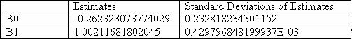
Table 17: Coefficient estimates for Norris(www.itl.nist.gov) - LREs : : 9,9 : 12,3 : 10,2
- LREs for SPSS v 7.5 : : 9,9 , : 12,3 , : 10,2 (McCullough, 1998)

Difficulty: Average
We used the dataset NoInt1 in order to test the performance in average difficulty dataset. Regression model is as follows:
y = B1*x + e
Certified Values for NoInt1 :
- Sample Residual Sum of Squares : 127,272727272727
- Coefficient estimate : 2.07438016528926, standard deviation : 0.16528925619834E-0(www.itl.nist.gov)
- LREs: :12,8 : 15 : 12,9
- LREs for SPSS v. 7.5 : : 12,8 , : 14,7 , : 12,5 (McCullough, 1998)
Difficulty: High
Our high level difficulty dataset is Longley designed by NIST.
- Model: y =B0+B1*x1 + B2*x2 + B3*x3 + B4*x4 + B5*x5 + B6*x6 +e
- LREs :
- : -log10 |836424,055505842-836424,055505915|/ |836424,055505915| = 13,1
- : 15
- : -log10 | 0,16528925619836E-01 – 0,16528925619834E-01|/ |0,16528925619834E-01| = 12,9
- LREs for SPSS v. 7.5 : : 12,8 , : 14,7 , : 12,5 (McCullough, 1998)
As we conclude from the computed LREs, there is no big difference between the results of two versions for linear regression.
Conclusion
editBy applying these test we try to find out whether the software are reliable and deliver accurate results or not. However based on the results we can say that different software packages deliver different results for same the problem which can lead us to wrong interpretations for statistical research questions.
In specific we can that SAS, SPSS and S-Plus can solve the linear regression problems better in comparision to ANOVA Problems. All three of them deliver poor results for F statistic calculation.
From the results of comparison two different versions of SPSS we can conclude that the difference between the accuracy of the results delivered by SPSS v.12 and v.7.5 is not great considering the difference between the version numbers. On the other hand SPSS v.12 can handle the ANOVA Problems much better than old version. However it has still problems in higher difficulty problems.
References
edit- McCullough, B.D. 1998, 'Assessing The Reliability of Ststistical Software: Part I',The American Statistician, Vol.52, No.4, pp.358-366.
- McCullough, B.D. 1999, 'Assessing The Reliability of Ststistical Software: Part II', The American Statistician, Vol.53, No.2, pp.149-159
- Sawitzki, G. 1994, 'Testing Numerical Reliability of Data Analysis Systems', Computational Statistics & Data Analysis, Vol.18, No.2, pp.269-286
- Wilkinson, L. 1993, 'Practical Guidelines for Testing Statistical Software' in 25th Conference on Statistical Computing at Schloss Reisenburg, ed. P. Dirschedl& R. Ostermnann, Physica Verlag
- National Institute of Standards and Technology. (1 September 2000). The Statistical Reference Datasets: Archives, [Online], Available from: <http://www.itl.nist.gov/div898/strd/general/dataarchive.html> [10 November 2005].