Sensory Systems/Visual System

Sensory Systems

Vision
Hearing
Balance
Feeling
Smell
Taste

Technological Aspects

Implants
Models

In Animals

Birds
Fish
Marine Animals
Arthropods
Other Animals

Introduction

Generally speaking, visual systems rely on electromagnetic (EM) waves to give an organism more information about its surroundings. This information could be regarding potential mates, dangers and sources of sustenance. Different organisms have different constituents that make up what is referred to as a visual system.

The complexity of eyes range from something as simple as an eye spot, which is nothing more than a collection of photosensitive cells, to a fully fledged camera eye. If an organism has different types of photosensitive cells, or cells sensitive to different wavelength ranges, the organism would theoretically be able to perceive colour or at the very least colour differences. Polarisation, another property of EM radiation, can be detected by some organisms, with insects and cephalopods having the highest accuracy.

Please note, in this text, the focus has been on using EM waves to see. Granted, some organisms have evolved alternative ways of obtaining sight or at the very least supplementing what they see with extra-sensory information. For example, whales or bats, which use echo-location. This may be seeing in some sense of the definition of the word, but it is not entirely correct. Additionally, vision and visual are words most often associated with EM waves in the visual wavelength range, which is normally defined as the same wavelength limits of human vision.

Electromagnetic spectrum

Since some organisms detect EM waves with frequencies below and above that of humans a better definition must be made. We therefore define the visual wavelength range as wavelengths of EM between 300nm and 800nm. This may seem arbitrary to some, but selecting the wrong limits would render parts of some bird's vision as non-vision. Also, with this range of wavelengths, we have defined for example the thermal-vision of certain organisms, like for example snakes as non-vision. Therefore snakes using their pit organs, which is sensitive to EM between 5000nm and 30,000nm (IR), do not "see", but somehow "feel" from afar. Even if blind specimens have been documented targeting and attacking particular body parts.

Firstly a brief description of different types of visual system sensory organs will be elaborated on, followed by a thorough explanation of the components in human vision, the signal processing of the visual pathway in humans and finished off with an example of the perceptional outcome due to these stages.

Sensory Organs

Vision, or the ability to see depends on visual system sensory organs or eyes. There are many different constructions of eyes, ranging in complexity depending on the requirements of the organism. The different constructions have different capabilities, are sensitive to different wave-lengths and have differing degrees of acuity, also they require different processing to make sense of the input and different numbers to work optimally. The ability to detect and decipher EM has proved to be a valuable asset to most forms of life, leading to an increased chance of survival for organisms that utilise it. In environments without sufficient light, or complete lack of it, lifeforms have no added advantage of vision, which ultimately has resulted in atrophy of visual sensory organs with subsequent increased reliance on other senses (e.g. some cave dwelling animals, bats etc.). Interestingly enough, it appears that visual sensory organs are tuned to the optical window, which is defined as the EM wavelengths (between 300nm and 1100nm) that pass through the atmosphere reaching to the ground. This is shown in the figure below. You may notice that there exists other "windows", an IR window, which explains to some extent the thermal-"vision" of snakes, and a radiofrequency (RF) window, of which no known lifeforms are able to detect.

Through time evolution has yielded many eye constructions, and some of them have evolved multiple times, yielding similarities for organisms that have similar niches. There is one underlying aspect that is essentially identical, regardless of species, or complexity of sensory organ type, the universal usage of light-sensitive proteins called opsins. Without focusing too much on the molecular basis though, the various constructions can be categorised into distinct groups:

• Spot Eyes

• Pit Eyes

• Pinhole Eyes

• Lens Eyes

• Refractive Cornea Eyes

• Reflector Eyes

• Compound Eyes

The least complicated configuration of eyes enable organisms to simply sense the ambient light, enabling the organism to know whether there is light or not. It is normally simply a collection of photosensitive cells in a cluster in the same spot, thus sometimes referred to as spot eyes, eye spot or stemma. By either adding more angular structures or recessing the spot eyes, an organisms gains access to directional information as well, which is a vital requirement for image formation. These so called pit eyes are by far the most common types of visual sensory organs, and can be found in over 95% of all known species.

Pinhole eye

Taking this approach to the obvious extreme leads to the pit becoming a cavernous structure, which increases the sharpness of the image, alas at a loss in intensity. In other words, there is a trade-off between intensity or brightness and sharpness. An example of this can be found in the Nautilus, species belonging to the family Nautilidae, organisms considered to be living fossils. They are the only known species that has this type of eye, referred to as the pinhole eye, and it is completely analogous to the pinhole camera or the camera obscura. In addition, like more advanced cameras, Nautili are able to adjust the size of the aperture thereby increasing or decreasing the resolution of the eye at a respective decrease or increase in image brightness. Like the camera, the way to alleviate the intensity/resolution trade-off problem is to include a lens, a structure that focuses the light unto a central area, which most often has a higher density of photo-sensors. By adjusting the shape of the lens and moving it around, and controlling the size of the aperture or pupil, organisms can adapt to different conditions and focus on particular regions of interest in any visual scene. The last upgrade to the various eye constructions already mentioned is the inclusion of a refractive cornea. Eyes with this structure have delegated two thirds of the total optic power of the eye to the high refractive index liquid inside the cornea, enabling very high resolution vision. Most land animals, including humans have eyes of this particular construct. Additionally, many variations of lens structure, lens number, photosensor density, fovea shape, fovea number, pupil shape etc. exists, always, to increase the chances of survival for the organism in question. These variations lead to a varied outward appearance of eyes, even with a single eye construction category. Demonstrating this point, a collection of photographs of animals with the same eye category (refractive cornea eyes) is shown below.

Refractive Cornea Eyes

Hawk Eye

Sheep Eye

Cat Eye

Human Eye

Crocodile Eye

An alternative to the lens approach called reflector eyes can be found in for example mollusks. Instead of the conventional way of focusing light to a single point in the back of the eye using a lens or a system of lenses, these organisms have mirror like structures inside the chamber of the eye that reflects the light into a central portion, much like a parabola dish. Although there are no known examples of organisms with reflector eyes capable of image formation, at least one species of fish, the spookfish (Dolichopteryx longipes) uses them in combination with "normal" lensed eyes.

Compound eye

The last group of eyes, found in insects and crustaceans, is called compound eyes. These eyes consist of a number of functional sub-units called ommatidia, each consisting of a facet, or front surface, a transparent crystalline cone and photo-sensitive cells for detection. In addition each of the ommatidia are separated by pigment cells, ensuring the incoming light is as parallel as possible. The combination of the outputs of each of these ommatidia form a mosaic image, with a resolution proportional to the number of ommatidia units. For example, if humans had compound eyes, the eyes would have covered our entire faces to retain the same resolution. As a note, there are many types of compound eyes, but delving to deep into this topic is beyond the scope of this text.

Not only the type of eyes vary, but also the number of eyes. As you are well aware of, humans usually have two eyes, spiders on the other hand have a varying number of eyes, with most species having 8. Normally the spiders also have varying sizes of the different pairs of eyes and the differing sizes have different functions. For example, in jumping spiders 2 larger front facing eyes, give the spider excellent visual acuity, which is used mainly to target prey. 6 smaller eyes have much poorer resolution, but helps the spider to avoid potential dangers. Two photographs of the eyes of a jumping spider and the eyes of a wolf spider are shown to demonstrate the variability in the eye topologies of arachnids.

• Eye Topologies of Spiders
• 
  Wolf Spider
• 
  Jumping Spider

Anatomy of the Visual System

We humans are visual creatures, therefore our eyes are complicated with many components. In this chapter, an attempt is made to describe these components, thus giving some insight into the properties and functionality of human vision.

Getting inside of the eyeball - Pupil, iris and the lens

Light rays enter the eye structure through the black aperture or pupil in the front of the eye. The black appearance is due to the light being fully absorbed by the tissue inside the eye. Only through this pupil can light enter into the eye which means the amount of incoming light is effectively determined by the size of the pupil. A pigmented sphincter surrounding the pupil functions as the eye's aperture stop. It is the amount of pigment in this iris, that give rise to the various eye colours found in humans.

In addition to this layer of pigment, the iris has 2 layers of ciliary muscles. A circular muscle called the pupillary sphincter in one layer, that contracts to make the pupil smaller. The other layer has a smooth muscle called the pupillary dilator, which contracts to dilate the pupil. The combination of these muscles can thereby dilate/contract the pupil depending on the requirements or conditions of the person. The ciliary muscles are controlled by ciliary zonules, fibres that also change the shape of the lens and hold it in place.

The lens is situated immediately behind the pupil. Its shape and characteristics reveal a similar purpose to that of camera lenses, but they function in slightly different ways. The shape of the lens is adjusted by the pull of the ciliary zonules, which consequently changes the focal length. Together with the cornea, the lens can change the focus, which makes it a very important structure indeed, however only one third of the total optical power of the eye is due to the lens itself. It is also the eye's main filter. Lens fibres make up most of the material for the lense, which are long and thin cells void of most of the cell machinery to promote transparency. Together with water soluble proteins called crystallins, they increase the refractive index of the lens. The fibres also play part in the structure and shape of the lens itself.

Schematic diagram of the human eye

Beamforming in the eye – Cornea and its protecting agent - Sclera

Structure of the Cornea

The cornea, responsible for the remaining 2/3 of the total optical power of the eye, covers the iris, pupil and lens. It focuses the rays that pass through the iris before they pass through the lens. The cornea is only 0.5mm thick and consists of 5 layers:

• Epithelium: A layer of epithelial tissue covering the surface of the cornea.
• Bowman's membrane: A thick protective layer composed of strong collagen fibres, that maintain the overall shape of the cornea.
• Stroma: A layer composed of parallel collagen fibrils. This layer makes up 90% of the cornea's thickness.
• Descemet's membrane and Endothelium: Are two layers adjusted to the anterior chamber of the eye filled with aqueous humor fluid produced by the ciliary body. This fluid moisturises the lens, cleans it and maintains the pressure in the eye ball. The chamber, positioned between cornea and iris, contains a trabecular meshwork body through which the fluid is drained out by Schlemm canal, through posterior chamber.

The surface of the cornea lies under two protective membranes, called the sclera and Tenon’s capsule. Both of these protective layers completely envelop the eyeball. The sclera is built from collagen and elastic fibres, which protect the eye from external damages, this layer also gives rise to the white of the eye. It is pierced by nerves and vessels with the largest hole reserved for the optic nerve. Moreover, it is covered by conjunctiva, which is a clear mucous membrane on the surface of the eyeball. This membrane also lines the inside of the eyelid. It works as a lubricant and, together with the lacrimal gland, it produces tears, that lubricate and protect the eye. The remaining protective layer, the eyelid, also functions to spread this lubricant around.

Moving the eyes – extra-ocular muscles

The eyeball is moved by a complicated muscle structure of extra-ocular muscles consisting of four rectus muscles – inferior, medial, lateral and superior and two oblique – inferior and superior. Positioning of these muscles is presented below, along with functions:

Extra-ocular muscles: Green - Lateral Rectus; Red - Medial Rectus; Cyan - Superior Rectus; Pink - Inferior Rectus; Dark Blue - Superior Oblique; Yellow - Inferior Oblique.

As you can see, the extra-ocular muscles (2,3,4,5,6,8) are attached to the sclera of the eyeball and originate in the annulus of Zinn, a fibrous tendon surrounding the optic nerve. A pulley system is created with the trochlea acting as a pulley and the superior oblique muscle as the rope, this is required to redirect the muscle force in the correct way. The remaining extra-ocular muscles have a direct path to the eye and therefore do not form these pulley systems. Using these extra-ocular muscles, the eye can rotate up, down, left, right and alternative movements are possible as a combination of these.

Other movements are also very important for us to be able to see. Vergence movements enable the proper function of binocular vision. Unconscious fast movements called saccades, are essential for people to keep an object in focus. The saccade is a sort of jittery movement performed when the eyes are scanning the visual field, in order to displace the point of fixation slightly. When you follow a moving object with your gaze, your eyes perform what is referred to as smooth pursuit. Additional involuntary movements called nystagmus are caused by signals from the vestibular system, together they make up the vestibulo-ocular reflexes.

The brain stem controls all of the movements of the eyes, with different areas responsible for different movements.

• Pons: Rapid horizontal movements, such as saccades or nystagmus
• Mesencephalon: Vertical and torsional movements
• Cerebellum: Fine tuning
• Edinger-Westphal nucleus: Vergence movements

Where the vision reception occurs – The retina

Filtering of the light performed by the cornea, lens and pigment epithelium

Before being transduced, incoming EM passes through the cornea, lens and the macula. These structures also act as filters to reduce unwanted EM, thereby protecting the eye from harmful radiation. The filtering response of each of these elements can be seen in the figure "Filtering of the light performed by cornea, lens and pigment epithelium". As one may observe, the cornea attenuates the lower wavelengths, leaving the higher wavelengths nearly untouched. The lens blocks around 25% of the EM below 400nm and more than 50% below 430nm. Finally, the pigment ephithelium, the last stage of filtering before the photo-reception, affects around 30% of the EM between 430nm and 500nm.

A part of the eye, which marks the transition from non-photosensitive region to photosensitive region, is called the ora serrata. The photosensitive region is referred to as the retina, which is the sensory structure in the back of the eye. The retina consists of multiple layers presented below with millions of photoreceptors called rods and cones, which capture the light rays and convert them into electrical impulses. Transmission of these impulses is nervously initiated by the ganglion cells and conducted through the optic nerve, the single route by which information leaves the eye.

Structure of retina including the main cell components: RPE: retinal pigment epithelium; OS: outer segment of the photoreceptor cells; IS: inner segment of the photoreceptor cells; ONL: outer nuclear layer; OPL: outer plexiform layer; INL: inner nuclear layer IPL: inner plexiform layer; GC: ganglion cell layer; P: pigment epithelium cell; BM: Bruch-Membran; R: rods; C: cones; H: horizontal cell; B: bipolar cell; M: Müller cell; A:amacrine cell; G: ganglion cell; AX: Axon; arrow: Membrane limitans externa.

A conceptual illustration of the structure of the retina is shown on the right. As we can see, there are five main cell types:

• photoreceptor cells
• horizontal cells
• bipolar cells
• amacrine cells
• ganglion cells

Photoreceptor cells can be further subdivided into two main types called rods and cones. Cones are much less numerous than rods in most parts of the retina, but there is an enormous aggregation of them in the macula, especially in its central part called the fovea. In this central region, each photo-sensitive cone is connected to one ganglion-cell. In addition, the cones in this region are slightly smaller than the average cone size, meaning you get more cones per area. Because of this ratio, and the high density of cones, this is where we have the highest visual acuity.

Distribution of Cones and Rods on Human Retina

There are 3 types of human cones, each of the cones responding to a specific range of wavelengths, because of three types of a pigment called photopsin. Each pigment is sensitive to red, blue or green wavelength of light, so we have blue, green and red cones, also called S-, M- and L-cones for their sensitivity to short-, medium- and long-wavelength respectively. It consists of protein called opsin and a bound chromphore called the retinal. The main building blocks of the cone cell are the synaptic terminal, the inner and outer segments, the interior nucleus and the mitochondria.

The spectral sensitivities of the 3 types of cones:

• 1. S-cones absorb short-wave light, i.e. blue-violet light. The maximum absorption wavelength for the S-cones is 420nm
• 2. M-cones absorb blue-green to yellow light. In this case The maximum absorption wavelength is 535nm
• 3. L-cones absorb yellow to red light. The maximum absorption wavelength is 565nm

Cone cell structure

The inner segment contains organelles and the cell's nucleus and organelles. The pigment is located in the outer segment, attached to the membrane as trans-membrane proteins within the invaginations of the cell-membrane that form the membranous disks, which are clearly visible in the figure displaying the basic structure of rod and cone cells. The disks maximize the reception area of the cells. The cone photoreceptors of many vertebrates contain spherical organelles called oil droplets, which are thought to constitute intra-ocular filters which may serve to increase contrast, reduce glare and lessen chromatic aberrations caused by the mitochondrial size gradient from the periphery to the centres.

Rods have a structure similar to cones, however they contain the pigment rhodopsin instead, which allows them to detect low-intensity light and makes them 100 times more sensitive than cones. Rhodopsin is the only pigment found in human rods, and it is found on the outer side of the pigment epithelium, which similarly to cones maximizes absorption area by employing a disk structure. Similarly to cones, the synaptic terminal of the cell joins it with a bipolar cell and the inner and outer segments are connected by cilium.

The pigment rhodopsin absorbs the light between 400-600nm, with a maximum absorption at around 500nm. This wavelength corresponds to greenish-blue light which means blue colours appear more intense in relation to red colours at night.

Rod cell structure

The sensitivity of cones and rods across visible EM

EM waves with wavelengths outside the range of 400 – 700 nm are not detected by either rods nor cones, which ultimately means they are not visible to human beings.

Horizontal cells occupy the inner nuclear layer of the retina. There are two types of horizontal cells and both types hyper-polarise in response to light i.e. they become more negative. Type A consists of a subtype called HII-H2 which interacts with predominantly S-cones. Type B cells have a subtype called HI-H1, which features a dendrite tree and an axon. The former contacts mostly M- and L-cone cells and the latter rod cells. Contacts with cones are made mainly by prohibitory synapses, while the cells themselves are joined into a network with gap junctions.

Cross-section of the human retina, with bipolar cells indicated in red.

Bipolar cells spread single dendrites in the outer plexiform layer and the perikaryon, their cell bodies, are found in the inner nuclear layer. Dendrites interconnect exclusively with cones and rods and we differentiate between one rod bipolar cell and nine or ten cone bipolar cells. These cells branch with amacrine or ganglion cells in the inner plexiform layer using an axon. Rod bipolar cells connect to triad synapses or 18-70 rod cells. Their axons spread around the inner plexiform layer synaptic terminals, which contain ribbon synapses and contact a pair of cell processes in dyad synapses. They are connected to ganglion cells with AII amacrine cell links.

Amecrine cells can be found in the inner nuclear layer and in the ganglion cell layer of the retina. Occasionally they are found in the inner plexiform layer, where they work as signal modulators. They have been classified as narrow-field, small-field, medium-field or wide-field depending on their size. However, many classifications exist leading to over 40 different types of amecrine cells.

Ganglion cells are the final transmitters of visual signal from the retina to the brain. The most common ganglion cells in the retina is the midget ganglion cell and the parasol ganglion cell. The signal after having passed through all the retinal layers is passed on to these cells which are the final stage of the retinal processing chain. All the information is collected here forwarded to the retinal nerve fibres and optic nerves. The spot where the ganglion axons fuse to create an optic nerve is called the optic disc. This nerve is built mainly from the retinal ganglion axons and Portort cells. The majority of the axons transmit data to the lateral geniculate nucleus, which is a termination nexus for most parts of the nerve and which forwards the information to the visual cortex. Some ganglion cells also react to light, but because this response is slower than that of rods and cones, it is believed to be related to sensing ambient light levels and adjusting the biological clock.

Signal Processing

As mentioned before the retina is the main component in the eye, because it contains all the light sensitive cells. Without it, the eye would be comparable to a digital camera without the CCD (Charge Coupled Device) sensor. This part elaborates on how the retina perceives the light, how the optical signal is transmitted to the brain and how the brain processes the signal to form enough information for decision making.

Creation of the initial signals - Photosensor Function

Vision invariably starts with light hitting the photo-sensitive cells found in the retina. Light-absorbing visual pigments, a variety of enzymes and transmitters in retinal rods and cones will initiate the conversion from visible EM stimuli into electrical impulses, in a process known as photoelectric transduction. Using rods as an example, the incoming visible EM hits rhodopsin molecules, transmembrane molecules found in the rods' outer disk structure. Each rhodopsin molecule consists of a cluster of helices called opsin that envelop and surround 11-cis retinal, which is the part of the molecule that will change due to the energy from the incoming photons. In biological molecules, moieties, or parts of molecules that will cause conformational changes due to this energy is sometimes referred to as chromophores. 11-cis retinal straightens in response to the incoming energy, turning into retinal (all-trans retinal), which forces the opsin helices further apart, causing particular reactive sites to be uncovered. This "activated" rhodopsin molecule is sometimes referred to as Metarhodopsin II. From this point on, even if the visible light stimulation stops, the reaction will continue. The Metarhodopsin II can then react with roughly 100 molecules of a G_s protein called transducing, which then results in a_s and ß? after the GDP is converted into GTP. The activated a_s-GTP then binds to cGMP-phosphodiesterase(PDE), suppressing normal ion-exchange functions, which results in a low cytosol concentration of cation ions, and therefore a change in the polarisation of the cell.

The natural photoelectric transduction reaction has an amazing power of amplification. One single retinal rhodopsin molecule activated by a single quantum of light causes the hydrolysis of up to 10⁶ cGMP molecules per second.

Photo Transduction

Representation of molecular steps in photoactivation (modified from Leskov et al., 2000). Depicted is an outer membrane disk in a rod. Step 1: Incident photon (hν) is absorbed and activates a rhodopsin by conformational change in the disk membrane to R*. Step 2: Next, R* makes repeated contacts with transducin molecules, catalyzing its activation to G* by the release of bound GDP in exchange for cytoplasmic GTP (Step 3). The α and γ subunit G* binds inhibitory γ subunits of the phosphodiesterase (PDE) activating its α and ß subunits. Step 4: Activated PDE hydrolyzes cGMP. Step 5: Guanylyl cyclase (GC) synthesizes cGMP, the second messenger in the phototransduction cascade. Reduced levels of cytosolic cGMP cause cyclic nucleotide gated channels to close preventing further influx of Na+ and Ca2+.

1. A light photon interacts with the retinal in a photoreceptor. The retinal undergoes isomerisation, changing from the 11-cis to all-trans configuration.
2. Retinal no longer fits into the opsin binding site.
3. Opsin therefore undergoes a conformational change to metarhodopsin II.
4. Metarhodopsin II is unstable and splits, yielding opsin and all-trans retinal.
5. The opsin activates the regulatory protein transducin. This causes transducin to dissociate from its bound GDP, and bind GTP, then the alpha subunit of transducin dissociates from the beta and gamma subunits, with the GTP still bound to the alpha subunit.
6. The alpha subunit-GTP complex activates phosphodiesterase.
7. Phosphodiesterase breaks down cGMP to 5'-GMP. This lowers the concentration of cGMP and therefore the sodium channels close.
8. Closure of the sodium channels causes hyperpolarization of the cell due to the ongoing potassium current.
9. Hyperpolarization of the cell causes voltage-gated calcium channels to close.
10. As the calcium level in the photoreceptor cell drops, the amount of the neurotransmitter glutamate that is released by the cell also drops. This is because calcium is required for the glutamate-containing vesicles to fuse with cell membrane and release their contents.
11. A decrease in the amount of glutamate released by the photoreceptors causes depolarization of On center bipolar cells (rod and cone On bipolar cells) and hyperpolarization of cone Off bipolar cells.

Without visible EM stimulation, rod cells containing a cocktail of ions, proteins and other molecules, have membrane potential differences of around -40mV. Compared to other nerve cells, this is quite high (-65mV). In this state, the neurotransmitter glutamate is continuously released from the axon terminals and absorbed by the neighbouring bipolar cells. With incoming visble EM and the previously mentioned cascade reaction, the potential difference drops to -70mV. This hyper-polarisation of the cell causes a reduction in the amount of released glutamate, thereby affecting the activity of the bipolar cells, and subsequently the following steps in the visual pathway.

Similar processes exist in the cone-cells and in photosensitive ganglion cells, but make use of different opsins. Photopsin I through III (yellowish-green, green and blue-violet respectively) are found in the three different cone cells and melanopsin (blue) can be found in the photosensitive ganglion cells.

Processing Signals in the Retina

Different bipolar cells react differently to the changes in the released glutamate. The so called ON and OFF bipolar cells are used to form the direct signal flow from cones to bipolar cells. The ON bipolar cells will depolarise by visible EM stimulation and the corresponding ON ganglion cells will be activated. On the other hand the OFF bipolar cells are hyper polarised by the visible EM stimulation, and the OFF ganglion cells are inhibited. This is the basic pathway of the Direct signal flow. The Lateral signal flow will start from the rods, then go to the bipolar cells, the amacrine cells, and the OFF bipolar cells inhibited by the Rod-amacrine cells and the ON bipolar cells will stimulated via an electrical synapse, after all of the previous steps, the signal will arrive at the ON or OFF ganglion cells and the whole pathway of the Lateral signal flow is established.

When the action potential (AP) in ON, ganglion cells will be triggered by the visible EM stimulus. The AP frequency will increase when the sensor potential increases. In other words, AP depends on the amplitude of the sensor's potential. The region of ganglion cells where the stimulatory and inhibitory effects influence the AP frequency is called receptive field (RF). Around the ganglion cells, the RF is usually composed of two regions: the central zone and the ring-like peripheral zone. They are distinguishable during visible EM adaptation. A visible EM stimulation on the centric zone could lead to AP frequency increase and the stimulation on the periphery zone will decrease the AP frequency. When the light source is turned off the excitation occurs. So the name of ON field (central field ON) refers to this kind of region. Of course the RF of the OFF ganglion cells act the opposite way and is therefore called "OFF field" (central field OFF). The RFs are organised by the horizontal cells. The impulse on the periphery region will be impulsed and transmitted to the central region, and there the so-called stimulus contrast is formed. This function will make the dark seem darker and the light brighter. If the whole RF is exposed to light. the impulse of the central region will predominate.

Signal Transmission to the Cortex

As mentioned previously, axons of the ganglion cells converge at the optic disk of the retina, forming the optic nerve. These fibres are positioned inside the bundle in a specific order. Fibres from the macular zone of the retina are in the central portion, and those from the temporal half of the retina take up the periphery part. A partial decussation or crossing occurs when these fibres are outside the eye cavity. The fibres from the nasal halves of each retina cross to the opposite halves and extend to the brain. Those from the temporal halves remain uncrossed. This partial crossover is called the optic chiasma, and the optic nerves past this point are called optic tracts, mainly to distinguish them from single-retinal nerves. The function of the partial crossover is to transmit the right-hand visual field produced by both eyes to the left-hand half of the brain only and vice versa. Therefore the information from the right half of the body, and the right visual field, is all transmitted to the left-hand part of the brain when reaches the posterior part of the fore-brain (diencephalon).

The pathway to the central cortex

The information relay between the fibers of optic tracts and the nerve cells occurs in the lateral geniculate bodies, the central part of the visual signal processing, located in the thalamus of the brain. From here the information is passed to the nerve cells in the occipital cortex of the corresponding side of the brain. Connections from the retina to the brain can be separated into a 'parvocellular pathway' and a "magnocellular pathway". The parvocellular pathways signals color and fine detail, whereas the magnocellular pathways detect fast moving stimuli.

Connections from the retina to the brain can be separated into a "parvocellular pathway" and a "magnocellular pathway". The parvocellular pathway originates in midget cells in the retina, and signals color and fine detail; magnocellular pathway starts with parasol cells, and detects fast moving stimuli.

Signals from standard digital cameras correspond approximately to those of the parvocellular pathway. To simulate the responses of parvocellular pathways, researchers have been developing neuromorphic sensory systems, which try to mimic spike-based computation in neural systems. Thereby they use a scheme called "address-event representation" for the signal transmission in the neuromorphic electronic systems (Liu and Delbruck 2010 [1]).

Anatomically, the retinal Magno and Parvo ganglion cells respectively project to 2 ventral magnocellular layers and 4 dorsal parvocellular layers of the Lateral Geniculate Nucleus (LGN). Each of the six LGN layers receives inputs from either the ipsilateral or contralateral eye, i.e., the ganglion cells of the left eye cross over and project to layer 1, 4 and 6 of the right LGN, and the right eye ganglion cells project (uncrossed) to its layer 2, 3 and 5. From here the information from the right and left eye is separated.

Although human vision is combined by two halves of the retina and the signal is processed by the opposite cerebral hemispheres, the visual field is considered as a smooth and complete unit. Hence the two visual cortical areas are thought of as being intimately connected. This connection, called corpus callosum is made of neurons, axons and dendrites. Because the dendrites make synaptic connections to the related points of the hemispheres, electric simulation of every point on one hemisphere indicates simulation of the interconnected point on the other hemisphere. The only exception to this rule is the primary visual cortex.

The synapses are made by the optic tract in the respective layers of the lateral geniculate body. Then these axons of these third-order nerve cells are passed up to the calcarine fissure in each occipital lobe of the cerebral cortex. Because bands of the white fibres and axons pair from the nerve cells in the retina go through it, it is called the striate cortex, which incidentally is our primary visual cortex, sometimes known as V1. At this point, impulses from the separate eyes converge to common cortical neurons, which then enables complete input from both eyes in one region to be used for perception and comprehension. Pattern recognition is a very important function of this particular part of the brain, with lesions causing problems with visual recognition or blindsight.

Based on the ordered manner in which the optic tract fibres pass information to the lateral geniculate bodies and after that pass in to the striate area, if one single point stimulation on the retina was found, the response which produced electrically in both lateral geniculate body and the striate cortex will be found at a small region on the particular retinal spot. This is an obvious point-to-point way of signal processing. And if the whole retina is stimulated, the responses will occur on both lateral geniculate bodies and the striate cortex gray matter area. It is possible to map this brain region to the retinal fields, or more usually the visual fields.

Any further steps in this pathway is beyond the scope of this book. Rest assured that, many further levels and centres exist, focusing on particular specific tasks, like for example colour, orientations, spatial frequencies, emotions etc.

Information Processing in the Visual System

Equipped with a firmer understanding of some of the more important concepts of the signal processing in the visual system, comprehension or perception of the processed sensory information is the last important piece in the puzzle. Visual perception is the process of translating information received by the eyes into an understanding of the external state of things. It makes us aware of the world around us and allows us to understand it better. Based on visual perception we learn patterns which we then apply later in life and we make decisions based on this and the obtained information. In other words, our survival depends on perception. The field of Visual Perception has been divided into different subfields, due to the fact that processing is too complex and requires of different specialized mechanisms to perceive what is seen. These subfields include: Color Perception, Motion Perception, Depth Perception, and Face Recognition, etc.

Deep Hierarchies in the Primate Visual Cortex

Deep hierarchies in the visual system

Despite the ever-increasing computational power of electronic systems, there are still many tasks where animals and humans are vastly superior to computers – one of them being the perception and contextualization of information. The classical computer, either the one in your phone or a supercomputer taking up the whole room, is in essence a number-cruncher. It can perform an incredible amount of calculations in a miniscule amount of time. What it lacks is creating abstractions of the information it is working with. If you attach a camera to your computer, the picture it “perceives” is just a grid of pixels, a 2-dimensional array of numbers. A human would immediately recognize the geometry of the scene, the objects in the picture, and maybe even the context of what’s going on. This ability of ours is provided by dedicated biological machinery – the visual system of the brain. It processes everything we see in a hierarchical way, starting from simpler features of the image to more complex ones all the way to classification of objects into categories. Hence the visual system is said to have a deep hierarchy. The deep hierarchy of the primate visual system has inspired computer scientists to create models of artificial neural networks that would also feature several layers where each of them creates higher generalizations of the input data.

Approximately half of the human neocortex is dedicated to vision. The processing of visual information happens over at least 10 functional levels. The neurons in the early visual areas extract simple image features over small local regions of visual space. As the information gets transmitted to higher visual areas, neurons respond to increasingly complex features. With higher levels of information processing the representations become more invariant – less sensitive to the exact feature size, rotation or position. In addition, the receptive field size of neurons in higher visual areas increases, indicating that they are tuned to more global image features. This hierarchical structure allows for efficient computing – different higher visual areas can use the same information computed in the lower areas. The generic scene description that is made in the early visual areas is used by other parts of the brain to complete various different tasks, such as object recognition and categorization, grasping, manipulation, movement planning etc.

Sub-cortical vision

The neural processing of visual information starts already before any of the cortical structures. Photoreceptors on the retina detect light and send signals to retinal ganglion cells. The receptive field size of a photoreceptor is one 100th of a degree (a one degree large receptive field is roughly the size of your thumb, when you have your arm stretched in front of you). The number of inputs to a ganglion cell and therefore its receptive field size depends on the location – in the center of the retina it receives signals from as few as five receptors, while in the periphery a single cell can have several thousand inputs. This implies that the highest spatial resolution is in the center of the retina, also called the fovea. Due to this property primates posses a gaze control mechanism that directs the eyesight so that the features of interest project onto the fovea.

Ganglion cells are selectively tuned to detect various features of the image, such as luminance contrast, color contrast, and direction and speed of movement. All of these features are the primary information used further up the processing pipeline. If there are visual stimuli that are not detectable by ganglion cells, then they are also not available for any cortical visual area.

Ganglion cells project to a region in thalamus called lateral geniculate nucleus (LGN), which in turn relays the signals to the cortex. There is no significant computation known to happen in LGN – there is almost a one-to-one correspondence between retinal ganglion and LGN cells. However, only 5% of the inputs to LGN come from the retina – all the other inputs are cortical feedback projections. Although the visual system is often regarded as a feed-forward system, the recurrent feedback connections as well as lateral connections are a common feature seen throughout the visual cortex. The role of the feedback is not yet fully understood but it is proposed to be attributed to processes like attention, expectation, imagination and filling-in the missing information.

Cortical vision

Main areas of the visual system

The visual cortex can be divided into three large parts – the occipital part which receives input from LGN and then sends outputs to dorsal and ventral streams. Occipital part includes the areas V1-V4 and MT, which process different aspects of visual information and gives rise to a generic scene representation. The dorsal pathway is involved in the analysis of space and in action planning. The ventral pathway is involved in object recognition and categorization.

V1 is the first cortical area that processes visual information. It is sensitive to edges, gratings, line-endings, motion, color and disparity (angular difference between the projections of a point onto the left and right retinas). The most straight forward example of the hierarchical bottom-up processing is the linear combination of the inputs from several ganglion cells with center-surround receptive fields to create a representation of a bar. This is done by the simple cells of V1 and was first described by the prominent neuroscientists Hubel and Wiesel. This type of information integration implies that the simple cells are sensitive to the exact location of the bar and have a relatively small receptive field. The complex cells of V1 receive inputs from the simple cells, and while also responding to linear oriented patterns they are not sensitive to the exact position of the bar and have a larger receptive field. The computation present in this step could be a MAX-like operation which produces responses similar in amplitude to the larger of the responses pertaining to the individual stimuli. Some simple and complex cells can also detect the end of a bar, and a fraction of V1 cells are also sensitive to local motion within their respective receptive fields.

Area V2 features more sophisticated contour representation including texture-defined contours, illusory contours and contours with border ownership. V2 also builds upon the absolute disparity detection in V1 and features cells that are sensitive to relative disparity which is the difference between the absolute disparities of two points in space. Area V4 receives inputs from V2 and area V3, but very little is known about the computation taking place in V3. Area V4 features neurons that are sensitive to contours with different curvature and vertices with particular angles. Another important feature is the coding for luminance-invariant hue. This is in contrast to V1 where neurons respond to color opponency along the two principle axis (red-green and yellow-blue) rather than the actual color. V4 further outputs to the ventral stream, to inferior temporal cortex (IT) which has been shown through lesion studies to be essential for object discrimination.

Inferior temporal cortex: object discrimination

Stimulus reduction in area TE

Inferior temporal cortex (IT) is divided into two areas: TEO and TE. Area TEO integrates information about the shapes and relative positions of multiple contour elements and features mostly cells which respond to simple combinations of features. The receptive field size of TEO neurons is about 3-5 degrees. Area TE features cells with significantly larger receptive fields (10-20 degrees) which respond to faces, hands and complex feature configurations. Cells in TE respond to visual features that are a simpler generalization of the object of interest but more complex than simple bars or spots. This was shown using a stimulus-reduction method by Tanaka et al. where first a response to an object is measured and then the object is replaced by simpler representations until the critical feature that the TE neurons are responding to is narrowed down.

It appears that the neurons in IT pull together various features of medium complexity from lower levels in the ventral stream to build models of object parts. The neurons in TE that are selective to specific objects have to fulfil two seemingly contradictory requirements – selectivity and invariance. They have to distinguish between different objects by the means of sensitivity to features in the retinal images. However, the same object can be viewed from different angles and distances at different light conditions yielding highly dissimilar retinal images of the same object. To treat all these images as equivalent, invariant features must be derived that are robust against certain transformations, such as changes in position, illumination, size on the retina etc. Neurons in area TE show invariance to position and size as well as to partial occlusion, position-in-depth and illumination direction. Rotation in depth has been shown to have the weakest invariance, with the exception if the object is a human face.

Object categories are not yet explicitly present in area TE – a neuron might typically respond to several but not all exemplars of the same category (e.g., images of trees) and it might also respond to exemplars of different categories (e.g., trees and non-trees). Object recognition and classification most probably involves sampling from a larger population of TE neurons as well as receiving inputs from additional brain areas, e.g., those that are responsible for understanding the context of the scene. Recent readout experiments have demonstrated that statistical classifiers (e.g. support vector machines) can be trained to classify objects based on the responses of a small number of TE neurons. Therefore, a population of TE neurons in principle can reliably signal object categories by their combined activity. Interestingly, there are also reports on highly selective neurons in medial temporal lobe that respond to very specific cues, e.g., to the tower of Pisa in different images or to a particular person’s face.

Learning in the Visual System

Learning can alter the visual feature selectivity of neurons, with the effect of learning becoming stronger at higher hierarchical levels. There is no known evidence on learning in the retina and also the orientation maps in V1 seem to be genetically largely predetermined. However, practising orientation identification improves orientation coding in V1 neurons, by increasing the slope of the tuning curve. Similar but larger effects have been seen in V4. In area TE relatively little visual training has noticeable physiological effects on visual perception, on a single cell level as well as in fMRI. For example, morphing two objects into each other increases their perceived similarity. Overall it seems that the even the adult visual cortex is considerably plastic, and the level of plasticity can be significantly increased, e.g., by administering specific drugs or by living in an enriched environment.

Deep Neural Networks

Similarly to the deep hierarchy of the primate visual system, deep learning architectures attempt to model high-level abstractions of the input data by using multiple levels of non-linear transformations. The model proposed by Hubel and Wiesel where information is integrated and propagated in a cascade from retina and LGN to simple cells and complex cells in V1 inspired the creation of one of the first deep learning architectures, the neocognitron – a multilayered artificial neural network model. It was used for different pattern recognition tasks, including the recognition of handwritten characters. However, it took a lot of time to train the network (in the order of days) and since its inception in the 1980s deep learning didn’t get much attention until the mid-2000s with the abundance of digital data and the invention of faster training algorithms. Deep neural networks have proved themselves to be very effective in tasks that not so long ago seemed possible only for humans to perform, such as recognizing the faces of particular people in photos, understanding human speech (to some extent) and translating text from foreign languages. Furthermore, they have proven to be of great assistance in industry and science to search for potential drug candidates, map real neural networks in the brain and predict the functions of proteins. It must be noted that deep learning is only very loosely inspired from the brain and is much more of an achievement of the field of computer science / machine learning than of neuroscience. The basic parallels are that the deep neural networks are composed of units that integrate information inputs in a non-linear manner (neurons) and send signals to each other (synapses) and that there are different levels of increasingly abstract representations of the data. The learning algorithms and mathematical descriptions of the “neurons” used in deep learning are very different from the actual processes taking place in the brain. Therefore, the research in deep learning, while giving a huge push to a more sophisticated artificial intelligence, can give only limited insights about the brain.

Example of a neuron with its main components.

Example of a base unit of the neural networks. In the example the activation function is a Rectified Linear Unit (ReLU), but there are also other possibilities, among which the sigmoid or the hyperbolic tangent. The bias changes the threshold of activation of the unit, and as such it is analogous to the value of the threshold for the action potential in the neuron.

Example of a deep neural network. Each square represents one unit as described in the image above.

References

Papers on the deep hierarchies in the visual system

• Kruger, N.; Janssen, P.; Kalkan, S.; Lappe, M.; Leonardis, A.; Piater, J.; Rodriguez-Sanchez, A. J.; Wiskott, L. (August 2013). "Deep Hierarchies in the Primate Visual Cortex: What Can We Learn for Computer Vision?". IEEE Transactions on Pattern Analysis and Machine Intelligence. 35 (8): 1847–1871. doi:10.1109/TPAMI.2012.272.
• Poggio, Tomaso; Riesenhuber, Maximilian (1 November 1999). Nature Neuroscience. 2 (11): 1019–1025. doi:doi:10.1038/14819. {{cite journal}}: Check |doi= value (help); Missing or empty |title= (help)

Stimulus reduction experiment

• Tanaka, Keiji (March 1996). "Inferotemporal Cortex and Object Vision". Annual Review of Neuroscience. 19 (1): 109–139. doi:10.1146/annurev.ne.19.030196.000545.

Evidence on learning in the visual system

• Li, Nuo; DiCarlo, James J. (23 September 2010). "Unsupervised Natural Visual Experience Rapidly Reshapes Size-Invariant Object Representation in Inferior Temporal Cortex". Neuron. 67 (6): 1062–1075. doi:10.1016/j.neuron.2010.08.029.
• Raiguel, S.; Vogels, R.; Mysore, S. G.; Orban, G. A. (14 June 2006). "Learning to See the Difference Specifically Alters the Most Informative V4 Neurons". Journal of Neuroscience. 26 (24): 6589–6602. doi:10.1523/JNEUROSCI.0457-06.2006.
• Schoups, A; Vogels, R; Qian, N; Orban, G (2 August 2001). "Practising orientation identification improves orientation coding in V1 neurons". Nature. 412 (6846): 549–53. PMID 11484056.

A recent and accessible overview of the status quo of the deep learning research

• Jones, Nicola (8 January 2014). "Computer science: The learning machines". Nature. 505 (7482): 146–148. doi:10.1038/505146a.

Motion Perception

Motion Perception is the process of inferring speed and direction of moving objects. Area V5 in humans and area MT (Middle Temporal) in primates are responsible for cortical perception of Motion. Area V5 is part of the extrastriate cortex, which is the region in the occipital region of the brain next to the primary visual cortex. The function of Area V5 is to detect speed and direction of visual stimuli, and integrate local visual motion signals into global motion. Area V1 or Primary Visual cortex is located in the occipital lobe of the brain in both hemispheres. It processes the first stage of cortical processing of visual information. This area contains a complete map of the visual field covered by the eyes. The difference between area V5 and area V1 (Primary Visual Cortex) is that area V5 can integrate motion of local signals or individual parts of an object into a global motion of an entire object. Area V1, on the other hand, responds to local motion that occurs within the receptive field. The estimates from these many neurons are integrated in Area V5.

Movement is defined as changes in retinal illumination over space and time. Motion signals are classified into First order motions and Second order motions. These motion types are briefly described in the following paragraphs.

Example of a "Beta movement".

First-order motion perception refers to the motion perceived when two or more visual stimuli switch on and off over time and produce different motion perceptions. First order motion is also termed "apparent motion,” and it is used in television and film. An example of this is the "Beta movement", which is an illusion in which fixed images seem to move, even though they do not move in reality. These images give the appearance of motion, because they change and move faster than what the eye can detect. This optical illusion happens because the human optic nerve responds to changes of light at ten cycles per second, so any change faster than this rate will be registered as a continuum motion, and not as separate images.

Second order motion refers to the motion that occurs when a moving contour is defined by contrast, texture, flicker or some other quality that does not result in an increase in luminance or motion energy of the image. Evidence suggests that early processing of First order motion and Second order motion is carried out by separate pathways. Second order mechanisms have poorer temporal resolution and are low-pass in terms of the range of spatial frequencies to which they respond. Second-order motion produces a weaker motion aftereffect. First and second-order signals are combined in are V5.

In this chapter, we will analyze the concepts of Motion Perception and Motion Analysis, and explain the reason why these terms should not be used interchangeably. We will analyze the mechanisms by which motion is perceived such as Motion Sensors and Feature Tracking. There exist three main theoretical models that attempt to describe the function of neuronal sensors of motion. Experimental tests have been conducted to confirm whether these models are accurate. Unfortunately, the results of these tests are inconclusive, and it can be said that no single one of these models describes the functioning of Motion Sensors entirely. However, each of these models simulates certain features of Motion Sensors. Some properties of these sensors are described. Finally, this chapter shows some motion illusions, which demonstrate that our sense of motion can be mislead by static external factors that stimulate motion sensors in the same way as motion.

Motion Analysis and Motion Perception

The concepts of Motion Analysis and Motion Perception are often confused as interchangeable. Motion Perception and Motion Analysis are important to each other, but they are not the same.

Motion Analysis refers to the mechanisms in which motion signals are processed. In a similar way in which Motion Perception does not necessarily depend on signals generated by motion of images in the retina, Motion Analysis may or may not lead to motion perception. An example of this phenomenon is Vection, which occurs when a person perceives that she is moving when she is stationary, but the object that she observes is moving. Vection shows that motion of an object can be analyzed, even though it is not perceived as motion coming from the object. This definition of Motion analysis suggests that motion is a fundamental image property. In the visual field, it is analyzed at every point. The results from this analysis are used to derive perceptual information.

Motion Perception refers to the process of acquiring perceptual knowledge about motion of objects and surfaces in an image. Motion is perceived either by delicate local sensors in the retina or by feature tracking. Local motion sensors are specialized neurons sensitive to motion, and analogous to specialized sensors for color. Feature tracking is an indirect way to perceive motion, and it consists of inferring motion from changes in retinal position of objects over time. It is also referred to as third order motion analysis. Feature tracking works by focusing attention to a particular object and observing how its position has changed over time.

Motion Sensors

Detection of motion is the first stage of visual processing, and it happens thanks to specialized neural processes, which respond to information regarding local changes of intensity of images over time. Motion is sensed independently of other image properties at all locations in the image. It has been proven that motion sensors exist, and they operate locally at all points in the image. Motion sensors are dedicated neuronal sensors located in the retina that are capable of detecting a motion produced by two brief and small light flashes that are so close together that they could not be detected by feature tracking. There exist three main models that attempt to describe the way that these specialized sensors work. These models are independent of one another, and they try to model specific characteristics of Motion Perception. Although there is not sufficient evidence to support that any of these models represent the way the visual system (motion sensors particularly) perceives motion, they still correctly model certain functions of these sensors.

Two different mechanisms for motion detection. Left) A "Reichardt detector" consists of two mirror-symmetrical subunits. In each subunit, the luminance values as measured in two adjacent points become multiplied (M) with each other after one of them is delayed by a low-pass filter with time-constant τ. The resulting output signals of the multipliers become finally subtracted. Right) In the gradient detector, the temporal luminance gradient as measured after one photoreceptor (δI/δt, Left) is divided by the spatial luminance gradient (δI/δx). Here, the spatial gradient is approximated by the difference between the luminance values in two adjacent points.

The Reichardt Detector

The Reichardt Detector is used to model how motion sensors respond to First order motion signals. When an objects moves from point A in the visual field to point B, two signals are generated: one before the movement began and another one after the movement has completed. This model perceives this motion by detecting changes in luminance at one point on the retina and correlating it with a change in luminance at another point nearby after a short delay. The Reichardt Detector operates based on the principle of correlation (statistical relation that involves dependency). It interprets a motion signal by spatiotemporal correlation of luminance signals at neighboring points. It uses the fact that two receptive fields at different points on the trajectory of a moving object receive a time shifted version of the same signal – a luminance pattern moves along an axis and the signal at one point in the axis is a time shifted version of a previous signal in the axis. The Reichardt Detector model has two spatially separate neighboring detectors. The output signals of the detectors are multiplied (correlated) in the following way: a signal multiplied by a second signal that is the time-shifted version of the original. The same procedure is repeated but in the reverse direction of motion (the signal that was time-shifted becomes the first signal and vice versa). Then, the difference between these two multiplications is taken, and the outcome gives the speed of motion. The response of the detector depends upon the stimulus’ phase, contrast and speed. Many detectors tuned at different speeds are necessary to encode the true speed of the pattern. The most compelling experimental evidence for this kind of detector comes from studies of direction discrimination of barely visible targets.

Motion-Energy Filtering

Motion Energy Filter is a model of Motion Sensors based on the principle of phase invariant filters. This model builds spatio-temporal filters oriented in space-time to match the structure of moving patterns. It consists of separable filters, for which spatial profiles remain the same shape over time but are scaled by the value of the temporal filters. Motion Energy Filters match the structure of moving patterns by adding together separable filters. For each direction of motion, two space-time filters are generated: one, which is symmetric (bar-like), and one which is asymmetric (edge-like). The sum of the squares of these filters is called the motion energy. The difference in the signal for the two directions is called the opponent energy. This result is then divided by the squared output of another filter, which is tuned to static contrast. This division is performed to take into account the effect of contrast in the motion. Motion Energy Filters can model a number of motion phenomenon, but it produces a phase independent measurement, which increases with speed but does not give a reliable value of speed.

Spatiotemporal Gradients

$v={\frac {dx}{dt}}=-{\frac {\frac {\partial I(x,t)}{\partial t}}{\frac {\partial I(x,t)}{\partial x}}}=-{\frac {D_{t}I}{D_{x}I}}$

This model of Motion sensors was originally developed in the field of computer vision, and it is based on the principle that the ratio of the temporal derivative of image brightness to the spatial derivative of image brightness gives the speed of motion. It is important to note that at the peaks and troughs of the image, this model will not compute an adequate answer, because the derivative in the denominator would be zero. In order to solve this problem, the first-order and higher-order spatial derivatives with respect to space and time can also be analyzed. Spatiotemporal Gradients is a good model for determining the speed of motion at all points in the image.

Motion Sensors are Orientation-Selective

One of the properties of Motion Sensors is orientation-selectivity, which constrains motion analysis to a single dimension. Motion sensors can only record motion in one dimension along an axis orthogonal to the sensor’s preferred orientation. A stimulus that contains features of a single orientation can only be seen to move in a direction orthogonal to the stimulus’ orientation. One-dimensional motion signals give ambiguous information about the motion of two-dimensional objects. A second stage of motion analysis is necessary in order to resolve the true direction of motion of a 2-D object or pattern. 1-D motion signals from sensors tuned to different orientations are combined to produce an unambiguous 2-D motion signal. Analysis of 2-D motion depends on signals from local broadly oriented sensors as well as on signals from narrowly oriented sensors.

Feature Tracking

Another way in which we perceive motion is through Feature Tracking. Feature Tracking consists of analyzing whether or not the local features of an object have changed positions, and inferring movement from this change. In this section, some features about Feature trackers are mentioned.

Feature trackers fail when a moving stimulus occurs very rapidly. Feature trackers have the advantage over Motion sensors that they can perceive movement of an object even if the movement is separated by intermittent blank intervals. They can also separate these two stages (movements and blank intervals). Motion sensors, on the other hand, would just integrate the blanks with the moving stimulus and see a continuous movement. Feature trackers operate on the locations of identified features. For that reason, they have a minimum distance threshold that matches the precision with which locations of features can be discriminated. Feature trackers do not show motion aftereffects, which are visual illusions that are caused as a result of visual adaptation. Motion aftereffects occur when, after observing a moving stimulus, a stationary object appears to be moving in the opposite direction of the previously observed moving stimulus. It is impossible for this mechanism to monitor multiple motions in different parts of the visual field and at the same time. On the other hand, multiple motions are not a problem for motion sensors, because they operate in parallel across the entire visual field.

Experiments have been conducted using the information above to reach interesting conclusions about feature trackers. Experiments with brief stimuli have shown that color patterns and contrast patterns at high contrasts are not perceived by feature trackers but by motion sensors. Experiments with blank intervals have confirmed that feature tracking can occur with blank intervals in the display. It is only at high contrast that motion sensors perceive the motion of chromatic stimuli and contrast patterns. At low contrasts feature trackers analyze the motion of both chromatic patterns and contrast envelopes and at high contrasts motion sensors analyze contrast envelopes. Experiments in which subjects make multiple motion judgments suggest that feature tracking is a process that occurs under conscious control and that it is the only way we have to analyze the motion of contrast envelopes in low-contrast displays. These results are consistent with the view that the motion of contrast envelopes and color patterns depends on feature tracking except when colors are well above threshold or mean contrast is high. The main conclusion of these experiments is that it is probably feature tracking that allows perception of contrast envelopes and color patterns.

Motion Illusions

As a consequence of the process in which Motion detection works, some static images might seem to us like they are moving. These images give an insight into the assumptions that the visual system makes, and are called visual illusions.

A famous Motion Illusion related to first order motion signals is the Phi phenomenon, which is an optical illusion that makes us perceive movement instead of a sequence of images. This motion illusion allows us to watch movies as a continuum and not as separate images. The phi phenomenon allows a group of frozen images that are changed at a constant speed to be seen as a constant movement. The Phi phenomenon should not be confused with the Beta Movement, because the former is an apparent movement caused by luminous impulses in a sequence, while the later one is an apparent movement caused by luminous stationary impulses.

Motion Illusions happen when Motion Perception, Motion Analysis and the interpretation of these signals are misleading, and our visual system creates illusions about motion. These illusions can be classified according to which process allows them to happen. Illusions are classified as illusions related to motion sensing, 2D integration, and 3D interpretation

The most popular illusions concerning motion sensing are four-stroke motion, RDKs and second order motion signals illusions. The most popular motion illusions concerning 2D integration are Motion Capture, Plaid Motion and Direct Repulsion. Similarly, the ones concerning 3D interpretation are Transformational Motion, Kinetic Depth, Shadow Motion, Biological Motion, Stereokinetic motion, Implicit Figure Motion and 2 Stroke Motion. There are far more Motion Illusions, and they all show something interesting regarding human Motion Detection, Perception and Analysis mechanisms. For more information, visit the following link: http://www.lifesci.sussex.ac.uk/home/George_Mather/Motion/

Open Problems

Although we still do not understand most of the specifics regarding Motion Perception, understanding the mechanisms by which motion is perceived as well as motion illusion can give the reader a good overview of the state of the art in the subject. Some of the open problems regarding Motion Perception are the mechanisms of formation of 3D images in global motion and the Aperture Problem.

Global motion signals from the retina are integrated to arrive at a 2 dimensional global motion signal; however, it is unclear how 3D global motion is formed. The Aperture Problem occurs because each receptive field in the visual system covers only a small piece of the visual world, which leads to ambiguities in perception. The aperture problem refers to the problem of a moving contour that, when observed locally, is consistent with different possibilities of motion. This ambiguity is geometric in origin - motion parallel to the contour cannot be detected, as changes to this component of the motion do not change the images observed through the aperture. The only component that can be measured is the velocity orthogonal to the contour orientation; for that reason, the velocity of the movement could be anything from the family of motions along a line in velocity space. This aperture problem is not only observed in straight contours, but also in smoothly curved ones, since they are approximately straight when observed locally. Although the mechanisms to solve the Aperture Problem are still unknown, there exist some hypothesis on how it could be solved. For example, it could be possible to resolve this problem by combining information across space or from different contours of the same object.

Conclusions

In this chapter, we introduced Motion Perception and the mechanisms by which our visual system detects motion. Motion Illusions showed how Motion signals can be misleading, and consequently lead to incorrect conclusions about motion. It is important to remember that Motion Perception and Motion Analysis are not the same. Motion Sensors and Feature trackers complement each other to make the visual system perceive motion.

Motion Perception is complex, and it is still an open area of research. This chapter describes models about the way that Motion Sensors function, and hypotheses about Feature trackers characteristics; however, more experiments are necessary to learn about the characteristics of these mechanisms and be able to construct models that resemble the actual processes of the visual system more accurately.

The variety of mechanisms of motion analysis and motion perception described in this chapter, as well as the sophistication of the artificial models designed to describe them demonstrate that there is much complexity in the way in which the cortex processes signals from the outside environment. Thousands of specialized neurons integrate and interpret pieces of local signals to form global images of moving objects in our brain. Understanding that so many actors and processes in our bodies must work in concert to perceive motion makes our ability to it all the more remarkable that we as humans are able to do it with such ease.

Color Perception

Introduction

Humans (together with primates like monkeys and gorillas) have the best color perception among mammals . Hence, it is not a coincidence that color plays an important role in a wide variety of aspects. For example, color is useful for discriminating and differentiating objects, surfaces, natural scenery, and even faces ,. Color is also an important tool for nonverbal communication, including that of emotion .

For many decades, it has been a challenge to find the links between the physical properties of color and its perceptual qualities. Usually, these are studied under two different approaches: the behavioral response caused by color (also called psychophysics) and the actual physiological response caused by it .

Here we will only focus on the latter. The study of the physiological basis of color vision, about which practically nothing was known before the second half of the twentieth century, has advanced slowly and steadily since 1950. Important progress has been made in many areas, especially at the receptor level. Thanks to molecular biology methods, it has been possible to reveal previously unknown details concerning the genetic basis for the cone pigments. Furthermore, more and more cortical regions have been shown to be influenced by visual stimuli, although the correlation of color perception with wavelength-dependent physiology activity beyond the receptors is not so easy to discern .

In this chapter, we aim to explain the basics of the different processes of color perception along the visual path, from the retina in the eye to the visual cortex in the brain. For anatomical details, please refer to Sec. "Anatomy of the Visual System" of this Wikibook.

Color Perception at the Retina

All colors that can be discriminated by humans can be produced by the mixture of just three primary (basic) colors. Inspired by this idea of color mixing, it has been proposed that color is subserved by three classes of sensors, each having a maximal sensitivity to a different part of the visible spectrum . It was first explicitly proposed in 1853 that there are three degrees of freedom in normal color matching . This was later confirmed in 1886 (with remarkably close results to recent studies , ).

These proposed color sensors are actually the so called cones (Note: In this chapter, we will only deal with cones. Rods contribute to vision only at low light levels. Although they are known to have an effect on color perception, their influence is very small and can be ignored here.) . Cones are of the two types of photoreceptor cells found in the retina, with a significant concentration of them in the fovea. The Table below lists the three types of cone cells. These are distinguished by different types of rhodopsin pigment. Their corresponding absorption curves are shown in the Figure below.

Table 1: General overview of the cone types found in the retina.

Name	Higher sensitivity to color	Absorption curve peak [nm]
S, SWS, B	Blue	420
M, MWS, G	Green	530
L, LWS, R	Red	560

Absorption curves for the different cones. Blue, green, and red represent the absorption of the S (420 nm), M (530 nm), and L (560 nm) cones, respectively.

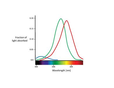
Although no consensus has been reached for naming the different cone types, the most widely utilized designations refer either to their action spectra peak or to the color to which they are sensitive themselves (red, green, blue). In this text, we will use the S-M-L designation (for short, medium, and long wavelength), since these names are more appropriately descriptive. The blue-green-red nomenclature is somewhat misleading, since all types of cones are sensitive to a large range of wavelengths.

An important feature about the three cone types is their relative distribution in the retina. It turns out that the S-cones present a relatively low concentration through the retina, being completely absent in the most central area of the fovea. Actually, they are too widely spaced to play an important role in spatial vision, although they are capable of mediating weak border perception . The fovea is dominated by L- and M-cones. The proportion of the two latter is usually measured as a ratio. Different values have been reported for the L/M ratio, ranging from 0.67 up to 2 , the latter being the most accepted. Why L-cones almost always outnumber the M-cones remains unclear. Surprisingly, the relative cone ratio has almost no significant impact on color vision. This clearly shows that the brain is plastic, capable of making sense out of whatever cone signals it receives , .

It is also important to note the overlapping of the L- and M-cone absorption spectra. While the S-cone absorption spectrum is clearly separated, the L- and M-cone peaks are only about 30 nm apart, their spectral curves significantly overlapping as well. This results in a high correlation in the photon catches of these two cone classes. This is explained by the fact that in order to achieve the highest possible acuity at the center of the fovea, the visual system treats L- and M-cones equally, not taking into account their absorption spectra. Therefore, any kind of difference leads to a deterioration of the luminance signal . In other words, the small separation between L- and M-cone spectra might be interpreted as a compromise between the needs for high-contrast color vision and high acuity luminance vision. This is congruent with the lack of S-cones in the central part of the fovea, where visual acuity is highest. Furthermore, the close spacing of L- and M-cone absorption spectra might also be explained by their genetic origin. Both cone types are assumed to have evolved "recently" (about 35 million years ago) from a common ancestor, while the S-cones presumably split off from the ancestral receptor much earlier.

The spectral absorption functions of the three different types of cone cells are the hallmark of human color vision. This theory solved a long-known problem: although we can see millions of different colors (humans can distinguish between 7 and 10 million different colors, our retinas simply do not have enough space to accommodate an individual detector for every color at every retinal location.

From the Retina to the Brain

The signals that are transmitted from the retina to higher levels are not simple point-wise representations of the receptor signals, but rather consist of sophisticated combinations of the receptor signals. The objective of this section is to provide a brief of the paths that some of this information takes.

Once the optical image on the retina is transduced into chemical and electrical signals in the photoreceptors, the amplitude-modulated signals are converted into frequency-modulated representations at the ganglion-cell and higher levels. In these neural cells, the magnitude of the signal is represented in terms of the number of spikes of voltage per second fired by the cell rather than by the voltage difference across the cell membrane. In order to explain and represent the physiological properties of these cells, we will find the concept of receptive fields very useful.

A receptive field is a graphical representation of the area in the visual field to which a given cell responds. Additionally, the nature of the response is typically indicated for various regions in the receptive field. For example, we can consider the receptive field of a photoreceptor as a small circular area representing the size and location of that particular receptor's sensitivity in the visual field. The Figure below shows exemplary receptive fields for ganglion cells, typically in a center-surround antagonism. The left receptive field in the figure illustrates a positive central response (know as on-center). This kind of response is usually generated by a positive input from a single cone surrounded by a negative response generated from several neighboring cones. Therefore, the response of this ganglion cell would be made up of inputs from various cones with both positive and negative signs. In this way, the cell not only responds to points of light, but serves as an edge (or more correctly, a spot) detector. In analogy to the computer vision terminology, we can think of the ganglion cell responses as the output of a convolution with an edge-detector kernel. The right receptive field of in the figure illustrates a negative central response (know as off-center), which is equally likely. Usually, on-center and off-center cells will occur at the same spatial location, fed by the same photoreceptors, resulting in an enhanced dynamic range.

The lower Figure shows that in addition to spatial antagonism, ganglion cells can also have spectral opponency. For instance, the left part of the lower figure illustrates a red-green opponent response with the center fed by positive input from an L-cone and the surrounding fed by a negative input from M-cones. On the other hand, the right part of the lower figure illustrates the off-center version of this cell. Hence, before the visual information has even left the retina, processing has already occurred, with a profound effect on color appearance. There are other types and varieties of ganglion cell responses, but they all share these basic concepts.

On center

Off center

Antagonist receptive fields

On center

Off center

Spectrally and spatially antagonist receptive fields.

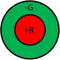
On their way to the primary visual cortex, ganglion cell axons gather to form the optic nerve, which projects to the lateral geniculate nucleus (LGN) in the thalamus. Coding in the optic nerve is highly efficient, keeping the number of nerve fibers to a minimum (limited by the size of the optic nerve) and thereby also the size of the retinal blind spot as small as possible (approximately 5° wide by 7° high). Furthermore, the presented ganglion cells would have no response to uniform illumination, since the positive and negative areas are balanced. In other words, the transmitted signals are uncorrelated. For example, information from neighboring parts of natural scenes are highly correlated spatially and therefore highly predictable . Lateral inhibition between neighboring retinal ganglion cells minimizes this spatial correlation, therefore improving efficiency. We can see this as a process of image compression carried out in the retina.

Given the overlapping of the L- and M-cone absorption spectra, their signals are also highly correlated. In this case, coding efficiency is improved by combining the cone signals in order to minimize said correlation. We can understand this more easily using Principal Component Analysis (PCA). PCA is a statistical method used to reduce the dimensionality of a given set of variables by transforming the original variables, to a set of new variables, the principal components (PCs). The first PC accounts for a maximal amount of total variance in the original variables, the second PC accounts for a maximal amount of variance that was not accounted for by the first component, and so on. In addition, PCs are linearly-independent and orthogonal to each other in the parameter space. PCA's main advantage is that only a few of the strongest PCs are enough to cover the vast majority of system variability . This scheme has been used with the cone absorption functions and even with the naturally occurring spectra,. The PCs that were found in the space of cone excitations produced by natural objects are 1) a luminance axis where the L- and M-cone signals are added (L+M), 2) the difference of the L- and M-cone signals (L-M), and 3) a color axis where the S-cone signal is differenced with the sum of the L- and M-cone signals (S-(L+M)). These channels, derived from a mathematical/computational approach, coincide with the three retino-geniculate channels discovered in electrophysiological experiments ,. Using these mechanisms, visual redundant information is eliminated in the retina.

There are three channels of information that actually communicate this information from the retina through the ganglion cells to the LGN. They are different not only on their chromatic properties, but also in their anatomical substrate. These channels pose important limitations for basic color tasks, such as detection and discrimination.

In the first channel, the output of L- and M-cones is transmitted synergistically to diffuse bipolar cells and then to cells in the magnocellular layers (M-) of the LGN (not to be confused with the M-cones of the retina). The receptive fields of the M-cells are composed of a center and a surround, which are spatially antagonist. M-cells have high-contrast sensitivity for luminance stimuli, but they show no response at some combination of L-M opponent inputs. However, because the null points of different M-cells vary slightly, the population response is never really zero. This property is actually passed on to cortical areas with predominant M-cell inputs.

The parvocellular pathway (P-) originates with the individual outputs from L- or M-cone to midget bipolar cells. These provide input to retinal P-cells. In the fovea, the receptive field centers of P-cells are formed by single L- or M-cones. The structure of the P-cell receptive field surround is still debated. However, the most accepted theory states that the surround consists of a specific cone type, resulting in a spatially opponent receptive field for luminance stimuli. Parvocellular layers contribute with about 80 % of the total projections from the retina to the LGN.

Finally, the recently discovered koniocellular pathway (K-) carries mostly signals from S-cones. Groups of this type of cones project to special bipolar cells, which in turn provide input to specific small ganglion cells. These are usually not spatially opponent. The axons of the small ganglion cells project to thin layers of the LGN (adjacent to parvocellular layers).

While the ganglion cells do terminate at the LGN (making synapses with LGN cells), there appears to be a one-to-one correspondence between ganglion cells and LGN cells. The LGN appears to act as a relay station for the signals. However, it probably serves some visual function, since there are neural projections from the cortex back to the LGN that could serve as some type of switching or adaptation feedback mechanism. The axons of LGN cells project to visual area one (V1) in the visual cortex in the occipital lobe.

Color Perception at the Brain

In the cortex, the projections from the magno-, parvo-, and koniocellular pathways end in different layers of the primary visual cortex. The magnocellular fibers innervate principally layer 4Cα and layer 6. Parvocellular neurons project mostly to 4Cβ, and layers 4A and 6. Koniocellular neurons terminate in the cytochrome oxidase (CO-) rich blobs in layers 1, 2, and 3.

Once in the visual cortex, the encoding of visual information becomes significantly more complex. In the same way the outputs of various photoreceptors are combined and compared to produce ganglion cell responses, the outputs of various LGN cells are compared and combined to produce cortical responses. As the signals advance further up in the cortical processing chain, this process repeats itself with a rapidly increasing level of complexity to the point that receptive fields begin to lose meaning. However, some functions and processes have been identified and studied in specific regions of the visual cortex.

In the V1 region (striate cortex), double opponent neurons - neurons that have their receptive fields both chromatically and spatially opposite with respect to the on/off regions of a single receptive field - compare color signals across the visual space . They constitute between 5 to 10% of the cells in V1. Their coarse size and small percentage matches the poor spatial resolution of color vision . Furthermore, they are not sensitive to the direction of moving stimuli (unlike some other V1 neurons) and, hence, unlikely to contribute to motion perception. However, given their specialized receptive field structure, these kind of cells are the neural basis for color contrast effects, as well as an efficient mean to encode color itself,. Other V1 cells respond to other types of stimuli, such as oriented edges, various spatial and temporal frequencies, particular spatial locations, and combinations of these features, among others. Additionally, we can find cells that linearly combine inputs from LGN cells as well as cells that perform nonlinear combination. These responses are needed to support advanced visual capabilities, such as color itself.

Fig. 4. (Partial) flow diagram illustrating the many streams of visual information processes that take place in the visual cortex. It is important to note that information can flow in both directions.

There is substantially less information on the chromatic properties of single neurons in V2 as compared to V1. On a first glance, it seems that there are no major differences of color coding in V1 and V2. One exception to this is the emergence of a new class of color-complex cell. Therefore, it has been suggested that V2 region is involved in the elaboration of hue. However, this is still very controversial and has not been confirmed.

Following the modular concept developed after the discovery of functional ocular dominance in V1, and considering the anatomical segregation between the P-, M-, and K-pathways (described in Sec. 3), it was suggested that a specialized system within the visual cortex devoted to the analysis of color information should exist. V4 is the region that has historically attracted the most attention as the possible "color area" of the brain. This is because of an influential study that claimed that V4 contained 100 % of hue-selective cells. However, this claim has been disputed by a number of subsequent studies, some even reporting that only 16 % of V4 neurons show hue tuning. Currently, the most accepted concept is that V4 contributes not only to color, but to shape perception, visual attention, and stereopsis as well. Furthermore, recent studies have focused on other brain regions trying to find the "color area" of the brain, such as TEO and PITd. The relationship of these regions to each other is still debated. To reconcile the discussion, some use the term posterior inferior temporal (PIT) cortex to denote the region that includes V4, TEO, and PITd.

If the cortical response in V1, V2, and V4 cells is already a very complicated task, the level of complexity of complex visual responses in a network of approximately 30 visual zones is humongous. Figure 4 shows a small portion of the connectivity of the different cortical areas (not cells) that have been identified.

At this stage, it becomes exceedingly difficult to explain the function of singles cortical cells in simple terms. As a matter of fact, the function of a single cell might not have meaning since the representation of various perceptions must be distributed across collections of cells throughout the cortex.

Color Vision Adaptation Mechanisms

Although researchers have been trying to explain the processing of color signals in the human visual system, it is important to understand that color perception is not a fixed process. Actually, there are a variety of dynamic mechanisms that serve to optimize the visual response according to the viewing environment. Of particular relevance to color perception are the mechanisms of dark, light, and chromatic adaptation.

Dark Adaptation

Dark adaptation refers to the change in visual sensitivity that occurs when the level of illumination is decreased. The visual system response to reduced illumination is to become more sensitive, increasing its capacity to produce a meaningful visual response even when the light conditions are suboptimal.

Fig. 5. Dark adaptation. During the first 10 minutes (i.e. to the left of the dotted line), sensitivity recovery is done by the cones. After the first 10 minutes (i.e. to the right of the dotted line), rods outperform the cones. Full sensitivity is recovered after approximately 30 minutes.

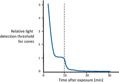
Figure 5 shows the recovery of visual sensitivity after transition from an extremely high illumination level to complete darkness. First, the cones become gradually more sensitive, until the curve levels off after a couple of minutes. Then, after approximately 10 minutes have passed, visual sensitivity is roughly constant. At that point, the rod system, with a longer recovery time, has recovered enough sensitivity to outperform the cones and therefore recover control the overall sensitivity. Rod sensitivity gradually improves as well, until it becomes asymptotic after about 30 minutes. In other words, cones are responsible for the sensitivity recovery for the first 10 minutes. Afterwards, rods outperform the cones and gain full sensitivity after approximately 30 minutes.

This is only one of several neural mechanisms produced in order to adapt to the dark lightning conditions as good as possible. Some other neural mechanisms include the well-known pupil reflex, depletion and regeneration of photopigment, gain control in retinal cells and other higher-level mechanisms, and cognitive interpretation, among others.

Light Adaptation

Light adaptation is essentially the inverse process of dark adaptation. As a matter of fact, the underlying physiological mechanisms are the same for both processes. However, it is important to consider it separately since its visual properties differ.

Fig. 6. Light adaptation. For a given scene, the solid lines represent families of visual response curves at different (relative) energy levels. The dashed line represents the case where we would adapt in order to cover the entire range of illumination, which would yield limited contrast and reduced sensitivity.

Light adaptation occurs when the level of illumination is increased. Therefore, the visual system must become less sensitive in order to produce useful perceptions, given the fact that there is significantly more visible light available. The visual system has a limited output dynamic range available for the signals that produce our perceptions. However, the real world has illumination levels covering at least 10 orders of magnitude more. Fortunately, we rarely need to view the entire range of illumination levels at the same time.

At high light levels, adaptation is achieved by photopigment bleaching. This scales photon capture in the receptors and protects the cone response from saturating at bright backgrounds. The mechanisms of light adaptation occur primarily within the retina. As a matter of fact, gain changes are largely cone-specific and adaptation pools signals over areas no larger than the diameter of individual cones,. This points to a localization of light adaptation that may be as early as the receptors. However, there appears to be more than one site of sensitivity scaling. Some of the gain changes are extremely rapid, while others take seconds or even minutes to stabilize. Usually, light adaptation takes around 5 minutes (six times faster than dark adaptation). This might point to the influence of post-receptive sites.

Figure 6 shows examples of light adaptation . If we would use a single response function to map the large range of intensities into the visual system's output, then we would only have a very small range at our disposal for a given scene. It is clear that with such a response function, the perceived contrast of any given scene would be limited and visual sensitivity to changes would be severely degraded due to signal-to-noise issues. This case is shown by the dashed line. On the other hand, solid lines represent families of visual responses. These curves map the useful illumination range in any given scene into the full dynamic range of the visual output, thus resulting in the best possible visual perception for each situation. Light adaptation can be thought of as the process of sliding the visual response curve along the illumination level axis until the optimum level for the given viewing conditions is reached.

Chromatic Adaptation

The general concept of chromatic adaptation consists in the variation of the height of the three cone spectral responsivity curves. This adjustment arises because light adaptation occurs independently within each class of cone. A specific formulation of this hypothesis is known as the von Kries adaptation. This hypothesis states that the adaptation response takes place in each of the three cone types separately and is equivalent to multiplying their fixed spectral sensitivities by a scaling constant. If the scaling weights (also known as von Kries coefficients) are inversely proportional to the absorption of light by each cone type (i.e. a lower absorption will require a larger coefficient), then von Kries scaling maintains a constant mean response within each cone class. This provides a simple yet powerful mechanism for maintaining the perceived color of objects despite changes in illumination. Under a number of different conditions, von Kries scaling provides a good account of the effects of light adaptation on color sensitivity and appearance,.

The easiest way to picture chromatic adaptation is by examining a white object under different types of illumination. For example, let's consider examining a piece of paper under daylight, fluorescent, and incandescent illumination. Daylight contains relatively far more short-wavelength energy than fluorescent light, and incandescent illumination contains relatively far more long-wavelength energy than fluorescent light. However, in spite of the different illumination conditions, the paper approximately retains its white appearance under all three light sources. This is because the S-cone system becomes relatively less sensitive under daylight (in order to compensate for the additional short-wavelength energy) and the L-cone system becomes relatively less sensitive under incandescent illumination (in order to compensate for the additional long-wavelength energy).

References

edit
- ↑ a b c d Conway, Bevil R (2009). "Color vision, cones, and color-coding in the cortex". The neuroscientist. 15: 274–290.
- ↑ Russell, Richard and Sinha, Pawan} (2007). "Real-world face recognition: The importance of surface reflectance properties". Perception. 36 (9).
{{cite journal}}: CS1 maint: multiple names: authors list (link) - ↑ Gegenfurtner, Karl R and Rieger, Jochem (2000). "Sensory and cognitive contributions of color to the recognition of natural scenes". Current Biology. 10 (13): 805–808.
{{cite journal}}: CS1 maint: multiple names: authors list (link) - ↑ Changizi, Mark A and Zhang, Qiong and Shimojo, Shinsuke (2006). "Bare skin, blood and the evolution of primate colour vision". Biology letters. 2 (2): 217–221.
{{cite journal}}: CS1 maint: multiple names: authors list (link) - ↑ a b Beretta, Giordano (2000). Understanding Color. Hewlett-Packard.
- ↑ a b Boynton, Robert M (1988). "Color vision". Annual review of psychology. 39 (1): 69–100.
- ↑ Grassmann, Hermann (1853). "Zur theorie der farbenmischung". Annalen der Physik. 165 (5): 69–84.
- ↑ Konig, Arthur and Dieterici, Conrad (1886). "Die Grundempfindungen und ihre intensitats-Vertheilung im Spectrum". Koniglich Preussischen Akademie der Wissenschaften.
{{cite journal}}: CS1 maint: multiple names: authors list (link) - ↑ Smith, Vivianne C and Pokorny, Joel (1975). "Spectral sensitivity of the foveal cone photopigments between 400 and 500 nm". Vision research. 15 (2): 161–171.
{{cite journal}}: CS1 maint: multiple names: authors list (link) - ↑ Vos, JJ and Walraven, PL (1971). "On the derivation of the foveal receptor primaries". Vision Research. 11 (8): 799–818.
{{cite journal}}: CS1 maint: multiple names: authors list (link) - ↑ a b c Gegenfurtner, Karl R and Kiper, Daniel C (2003). "Color vision". Neuroscience. 26 (1): 181.
{{cite journal}}: CS1 maint: multiple names: authors list (link) - ↑ Kaiser, Peter K and Boynton, Robert M (1985). "Role of the blue mechanism in wavelength discrimination". Vision research. 125 (4): 523–529.
{{cite journal}}: CS1 maint: multiple names: authors list (link) - ↑ Paulus, Walter and Kroger-Paulus, Angelika (1983). "A new concept of retinal colour coding". Vision research. 23 (5): 529–540.
{{cite journal}}: CS1 maint: multiple names: authors list (link) - ↑ Nerger, Janice L and Cicerone, Carol M (1992). "The ratio of L cones to M cones in the human parafoveal retina". Vision research. 32 (5): 879–888.
{{cite journal}}: CS1 maint: multiple names: authors list (link) - ↑ Neitz, Jay and Carroll, Joseph and Yamauchi, Yasuki and Neitz, Maureen and Williams, David R (2002). "Color perception is mediated by a plastic neural mechanism that is adjustable in adults". Neuron. 35 (4): 783–792.
{{cite journal}}: CS1 maint: multiple names: authors list (link) - ↑ Jacobs, Gerald H and Williams, Gary A and Cahill, Hugh and Nathans, Jeremy (2007). "Emergence of novel color vision in mice engineered to express a human cone photopigment". Science. 315 (5819): 1723–1725.
{{cite journal}}: CS1 maint: multiple names: authors list (link) - ↑ Osorio, D and Ruderman, DL and Cronin, TW (1998). "Estimation of errors in luminance signals encoded by primate retina resulting from sampling of natural images with red and green cones". JOSA A. 15 (1): 16–22.
{{cite journal}}: CS1 maint: multiple names: authors list (link) - ↑ Kersten, Daniel (1987). "Predictability and redundancy of natural images". JOSA A. 4 (112): 2395–2400.
- ↑ Jolliffe, I. T. (2002). Principal Component Analysis. Springer.
- ↑ Buchsbaum, Gershon and Gottschalk, A (1983). "Trichromacy, opponent colours coding and optimum colour information transmission in the retina". Proceedings of the Royal society of London. Series B. Biological sciences. 220 (1218): 89–113.
{{cite journal}}: CS1 maint: multiple names: authors list (link) - ↑ Zaidi, Qasim (1997). "Decorrelation of L-and M-cone signals". JOSA A. 14 (12): 3430–3431.
- ↑ Ruderman, Daniel L and Cronin, Thomas W and Chiao, Chuan-Chin (1998). "Statistics of cone responses to natural images: Implications for visual coding". JOSA A. 15 (8): 2036–2045.
{{cite journal}}: CS1 maint: multiple names: authors list (link) - ↑ Lee, BB and Martin, PR and Valberg, A (1998). "The physiological basis of heterochromatic flicker photometry demonstrated in the ganglion cells of the macaque retina". The Journal of Physiology. 404 (1): 323–347.
{{cite journal}}: CS1 maint: multiple names: authors list (link) - ↑ a b Derrington, Andrew M and Krauskopf, John and Lennie, Peter (1984). "Chromatic mechanisms in lateral geniculate nucleus of macaque". The Journal of Physiology. 357 (1): 241–265.
{{cite journal}}: CS1 maint: multiple names: authors list (link) - ↑ Shapley, Robert (1990). "Visual sensitivity and parallel retinocortical channels". Annual review of psychology. 41 (1): 635--658.
- ↑ Dobkins, Karen R and Thiele, Alex and Albright, Thomas D (2000). "Comparison of red--green equiluminance points in humans and macaques: evidence for different L: M cone ratios between species". JOSA A. 17 (3): 545–556.
{{cite journal}}: CS1 maint: multiple names: authors list (link) - ↑ Martin, Paul R and Lee, Barry B and White, Andrew JR and Solomon, Samuel G and Ruttiger, Lukas (2001). "Chromatic sensitivity of ganglion cells in the peripheral primate retina". Nature. 410 (6831): 933–936.
{{cite journal}}: CS1 maint: multiple names: authors list (link) - ↑ Perry, VH and Oehler, R and Cowey, A (1984). "Retinal ganglion cells that project to the dorsal lateral geniculate nucleus in the macaque monkey". Neuroscience. 12 (4): 1101--1123.
{{cite journal}}: Cite has empty unknown parameter:|month=(help)CS1 maint: multiple names: authors list (link) - ↑ Casagrande, VA (1994). "A third parallel visual pathway to primate area V1". Trends in neurosciences. 17 (7): 305–310.
- ↑ Hendry, Stewart HC and Reid, R Clay (2000). "The koniocellular pathway in primate vision". Annual review of neuroscience. 23 (1): 127–153.
{{cite journal}}: CS1 maint: multiple names: authors list (link) - ↑ Callaway, Edward M (1998). "Local circuits in primary visual cortex of the macaque monkey". Annual review of neuroscience. 21 (1): 47–74.
- ↑ Conway, Bevil R (2001). "Spatial structure of cone inputs to color cells in alert macaque primary visual cortex (V-1)". The Journal of Neuroscience. 21 (8): 2768–2783.
{{cite journal}}: Cite has empty unknown parameter:|month=(help) - ↑ Horwitz, Gregory D and Albright, Thomas D (2005). "Paucity of chromatic linear motion detectors in macaque V1". Journal of Vision. 5 (6).
{{cite journal}}: CS1 maint: multiple names: authors list (link) - ↑ Danilova, Marina V and Mollon, JD (2006). "The comparison of spatially separated colours". Vision research. 46 (6): 823–836.
{{cite journal}}: CS1 maint: multiple names: authors list (link) - ↑ Wachtler, Thomas and Sejnowski, Terrence J and Albright, Thomas D (2003). "Representation of color stimuli in awake macaque primary visual cortex". Neuron. 37 (4): 681–691.
{{cite journal}}: CS1 maint: multiple names: authors list (link) - ↑ Solomon, Samuel G and Lennie, Peter (2005). "Chromatic gain controls in visual cortical neurons". The Journal of neuroscience. 25 (19): 4779–4792.
{{cite journal}}: CS1 maint: multiple names: authors list (link) - ↑ Hubel, David H (1995). Eye, brain, and vision. Scientific American Library/Scientific American Books.
- ↑ Livingstone, Margaret S and Hubel, David H (1987). "Psychophysical evidence for separate channels for the perception of form, color, movement, and depth". The Journal of Neuroscience. 7 (11): 3416–3468.
{{cite journal}}: CS1 maint: multiple names: authors list (link) - ↑ Zeki, Semir M (1973). "Colour coding in rhesus monkey prestriate cortex". Brain research. 53 (2): 422–427.
- ↑ Conway, Bevil R and Tsao, Doris Y (2006). "Color architecture in alert macaque cortex revealed by fMRI". Cerebral Cortex. 16 (11): 1604–1613.
{{cite journal}}: CS1 maint: multiple names: authors list (link) - ↑ Tootell, Roger BH and Nelissen, Koen and Vanduffel, Wim and Orban, Guy A (2004). "Search for color 'center(s)'in macaque visual cortex". Cerebral Cortex. 14 (4): 353–363.
{{cite journal}}: CS1 maint: multiple names: authors list (link) - ↑ Conway, Bevil R and Moeller, Sebastian and Tsao, Doris Y (2007). "Specialized color modules in macaque extrastriate cortex". 560--573. 56 (3): 560–573.
{{cite journal}}: CS1 maint: multiple names: authors list (link) - ↑ a b c d Fairchild, Mark D (2013). Color appearance models. John Wiley & Sons.
- ↑ Webster, Michael A (1996). "Human colour perception and its adaptation". Network: Computation in Neural Systems. 7 (4): 587–634.
- ↑ Shapley, Robert and Enroth-Cugell, Christina (1984). "Visual adaptation and retinal gain controls". Progress in retinal research. 3: 263–346.
{{cite journal}}: CS1 maint: multiple names: authors list (link) - ↑ Chaparro, A and Stromeyer III, CF and Chen, G and Kronauer, RE (1995). "Human cones appear to adapt at low light levels: Measurements on the red-green detection mechanism". Vision Research. 35 (22): 3103–3118.
{{cite journal}}: CS1 maint: multiple names: authors list (link) - ↑ Macleod, Donald IA and Williams, David R and Makous, Walter (1992). "A visual nonlinearity fed by single cones". Vision research. 32 (2): 347–363.
{{cite journal}}: CS1 maint: multiple names: authors list (link) - ↑ Hayhoe, Mary (1991). Adaptation mechanisms in color and brightness. Springer.
- ↑ MacAdam, DAvid L (1970). Sources of Color Science. MIT Press.
- ↑ Webster, Michael A and Mollon, JD (1995). "Colour constancy influenced by contrast adaptation". Nature. 373 (6516): 694–698.
{{cite journal}}: CS1 maint: multiple names: authors list (link) - ↑ Brainard, David H and Wandell, Brian A (1992). "Asymmetric color matching: how color appearance depends on the illuminant". JOSA A. 9 (9): 1443–1448.
{{cite journal}}: CS1 maint: multiple names: authors list (link)