Pictures of Julia and Mandelbrot Sets/Print Version

Foreword

About This Book

This Wikibook deals with the production of pictures of Julia and Mandelbrot sets. Julia sets and Mandelbrot sets are very well-defined concepts. The most natural way of colouring is by using the potential function, though it is not actually the method most usually used. The book explains how to make pictures that are completely faultless in this regard. All the necessary theory is explained, all the formulas are stated and some words are said about how to put the things into a computer program.

The subject is primary pictures of Julia and Mandelbrot sets in their "pure" form, that is, without artificial intervention in the formula or in the colouring. Exceptions to this rule are techniques such as field lines, landscapes and critical systems for non-complex functions, that appeal to artistic utilization.

The book should not contain theory that has nothing to do with the pictures. Nor should it contain mathematical proofs. For our purposes faultless pictures are enough evidence of correct formulas, because the slightest error in a formula generally leads to serious errors in the picture.

If you find that something in this book ought to be explained in more details, you can either develop it further yourselves or advertise for that on the discussion page.

If you add a new picture or replace an illustration by a new one, it should be of best possible quality and have a size of about 800 pixels. Draw it twice or four times as large and diminish it.

Julia and Mandelbrot sets

Julia sets depend on a Rational Function

If a complex rational function is entered in the computer program and submitted to a certain iterative procedure, you get a colouring of the plane called a Julia set (although it is the domain outside the Julia set that is coloured). However, in order to get a picture that has aesthetic value the function must have a certain nature. It must either be constructed in a specific way to ensure that the picture is interesting, or it must contain a parameter, a complex number, that can vary. Being able to vary a parameter increases our chances of finding an interesting Julia sets for some value of the parameter.

What do we mean by 'interesting'? Essentially that the iterative procedure behaves in a somewhat chaotic way. If the iterative procedure's behaviour at each point is easily predicted for a particular function by behaviour of nearby points, then the Julia set for that function is not very crinkly, and rather uninteresting.

A Mandelbrot set is an Atlas to the Related Julia sets

If we vary the parameter in our rational function we can produce a kind of 'map' of values that lead to interesting Julia sets. Values of the complex parameter correspond to points in the plane. The set of points that lead to interesting Julia sets gives us some information about the structure of the Julia sets for the parameter value at each point. Such a set is called a Mandelbrot set. The Mandelbrot set can be regarded as an atlas of the Julia sets.

The difference between the Mandelbrot set for the family and "its" Julia sets, is that the structure of the Mandelbrot set varies from locality to locality, while a Julia set is self-similar: the different localities are transformations of each other.

Sometimes you will prefer the more complex picture of the varying structure of the Mandelbrot set. Sometimes you will prefer the pure structure of the Julia set. Sometimes you will draw the Julia set because the drawing of the Mandelbrot set is slow for certain functions.

The Julia set and the Fatou domains

Let $f(z)$ be a differentiable mapping from the complex plane $\mathbb {C}$ into itself. We assume first that $f(z)$ is differentiable as a complex function, that is, that $f(z)$ is a holomorphic function and therefore differentiable as many times as we like. Moreover we assume that $f(z)$ is rational, that is, $f(z)=p(z)/q(z)$, where both $p(z)$ and $q(z)$ are complex polynomials. If the degrees of $p(z)$ and $q(z)$ are m and n, respectively, we call d = m - n the degree of $f(z)$.

The theory of the Julia sets starts with this question: what can happen when we iterate a point z, that is, what happens when we form the sequence $z_{k}$ (k = 0, 1, 2, ...) where $z_{k+1}=f(z_{k})$ and $z_{0}=z$.

The three possibilities

Each sequence of iteration falls within one of these three classes:

1: The sequence converges towards a finite cycle of points, and all the points within a sufficiently small neighbourhood of z converge towards the same cycle.

2: The sequence goes into a finite cycle of (finite) polygon shaped or (infinite) annular shaped revolving movements, and all the points within a sufficiently small neighbourhood of z go into similar but concentrically lying movements.

3: The sequence goes into a finite cycle, but z is isolated having this property, or: for all the points w within a sufficiently small neighbourhood of z, the distance between the iterations of z and w is larger than the distance between z and w.

In the first case the cycle is attracting, in the second it is neutral (in this case there is a finite cycle which is centre for the movements) and in the third case the sequence of iteration is repelling.

Five Fatou domains

One Fatou domain

The set of points z, whose sequences of iteration converge to the same attracting cycle or go into the same neutral cycle, is an open set called a Fatou domain of $f(z)$. The complement to the union of these domains (the points satisfying condition 3) is a closed set called the Julia set of $f(z)$.

The Julia set is always non-empty and uncountable, and it is infinitely thin (without interior points). It is left invariant by $f(z)$, and here the sequences of iteration behave chaotically (apart from a countable number of points whose sequence is finite). The Julia set can be a simple curve, but it is usually a fractal.

The mean theorem on iteration of a complex rational function is:

Each of the Fatou domains has the same boundary

The common boundary is consequently the Julia set. This means that each point of the Julia set is a point of accumulation for each of the Fatou domains.

If there are more than two Fatou domains, we can infer that the Julia set must be a fractal, because each point of the Julia set has points of more than two different open sets infinitely close, but this is "impossible" since the plane is only two-dimensional.

Therefore, if we construct $f(z)$ in a particular way, we can know for certain that the Julia set is a fractal. This is the case for Newton iteration for solving an equation $g(z)=0$. Here $f(z)=z-g(z)/g'(z)$ and the solutions (that can be found by iteration) belong to different Fatou domains (consisting of the points iterating to that solution). The first picture shows the Julia set for the Newton iteration for $g(z)=z^{5}-1$. But a Julia set can be a fractal for other reasons, the next picture shows a Julia set for an iteration of the form $1000(1-z)/(8-4z+2z^{2}-z^{3})+c$, and here there is only one Fatou domain.

The critical points

To begin with, we must find all the Fatou domains. As a Fatou domain is determined if we know a single point in it, we must find a set of points such that each Fatou domain contains at least one of these. This is easily done, because:

Each of the Fatou domains contains at least one critical point of $f(z)$

A critical point of $f(z)$ is a (finite) point z satisfying $f'(z)=0$, or z = ∞, if the degree d of $f(z)$ is at least two, or if $f(z)=1/g(z)+c$ for some c and a rational function $g(z)$ satisfying this condition.

As we have presupposed that f(z) is rational, this means that there is only a finite number of Fatou domains.

We can find the solutions to $f'(z)=0$ by Newton iteration: if z* is a solution, a point near z* is iterated towards z* by $z$ → $z-f'(z)/f''(z)$. We can apply Newton iteration on a large number of regularly situated points in the plane, and register the different critical points (if the start point belongs to the Julia set of the iteration, it doesn't necessarily lead to a solution, likewise, we cannot be completely sure that we will catch all critical points, but for our task we should not care about this).

Here we will only deal with the attracting Fatou domains: a neutral domain cannot be coloured in a natural way, and unless $f(z)$ is particularly chosen, it is improbable in practice that the Fatou domain is neutral.

We can find the different attracting Fatou domains in the following way: We iterate each of the critical points a large number of times (or stop if the iterated point is numerically larger than a given large number), so that the iterated point z* is very near its terminus, which is possibly a cycle containing ∞, and we continue the iteration until the point is very near z* again. The number r(z*) of iterations needed for this is the order of the cycle. Hereafter we register the different cycles by removing the points z* belonging to a formerly registered cycle. This set of points corresponds to the set of Fatou domains.

A Fatou domain can contain several critical points, and from the number of the critical points in the Fatou domains we can say something about the connectedness of the Julia set: the fewer critical points in the Fatou domains, the more connected the Julia set.

The attraction of the cycle

In order to colour a Fatou domain in a natural and smooth way, besides the order of the cycle we must know its attraction $\alpha$ - a real number > 1:

For iteration towards an attracting cycle of order r, we have that if z* is a point of the cycle, then $f(f(...f(z*)))=z*$ (the r-fold composition), and the attraction is the number $\alpha =1/|(d(f(f(...f(z))))/dz)_{z=z*}|$. Note that $(d(f(f(...f(z))))/dz)_{z=z*}$ = the product of $f'(z_{i})$ for the r points of the cycle. If w is a point very near z* and $w_{r}$ is w iterated r times, we have that $\alpha =$lim_w→z*$|w-z*|/|w_{r}-z*|$.

However, this number $\alpha$ can be ∞, namely if the cycle contains a critical point (meaning that the critical point is iterated into itself after r iterations), and in this case the Fatou domain (and the cycle) is called super-attracting. We now set $\alpha =$lim_w→z*$log|w_{r}-z*|/log|w-z*|$ or $\alpha =$lim_w→∞$log|w_{r}|/log|w|$ if z* = ∞.

In the last case, that is, ∞ being a critical point and belonging to the cycle, we have |d| > 1 and $\alpha =|d|^{r}$. In this case we assume that ∞ is a fixed point (r = 1), so that d ≥ 2 and $\alpha =d$ (we thus ignore a function such as $1/(z-c)^{2}+c$, for which the attracting cycle is {c, ∞}).

In a case using Newton iteration to solve an equation $g(z)=0$ (so that $f(z)=z-g(z)/g'(z)$), the Fatou domains (containing a solution) are super-attracting, and $\alpha =2$ (if the solution is not a multiple root).

Colouring the Fatou domains

Our method of colouring is based on the real iteration number, which is connected with the potential function $\phi (z)$ of the Fatou domain. In the three cases the potential function is given by:

$\phi (z)=$lim_k→∞$1/(|z_{kr}-z*|\alpha ^{k})$ (non-super-attraction)

$\phi (z)=$lim_k→∞$log(1/|z_{kr}-z*|)/\alpha ^{k}$ (super-attraction)

$\phi (z)=$lim_k→∞$log|z_{k}|/d^{k}$ (d ≥ 2 and z* = ∞)

The real iteration number depends on the choice of a very small number $\epsilon$ (for iteration towards a finite cycle) and a very large number N (e.g. 10¹⁰⁰, for iteration towards ∞), and the sequence generated by z is set to stop when either $|z_{k}-z*|<\epsilon$ for one of the points z* (corresponding to the Fatou domains) or $|z_{k}|>N$, or when a chosen maximum number M of iterations is reached (which means that we have hit the Julia set, although this is not very probable).

If the cycle is not a fixed point, we must divide the iteration number k by the order r of the cycle, and take the integral part of this number.

Nice play of colours

If we calculate $\phi (z)$ for the k that stops the iteration, and replace $|z_{k}-z*|$ or $|z_{k}|$ by $\epsilon$ or N, respectively, we must replace the iteration number k by a real number, and this is the real iteration number. It is found by subtracting from k a number in the interval [0, 1[, and in the three cases this is given by:

$log(\epsilon /|z_{k}-z*|)/log(\alpha )$ (non-super-attraction)

$log(log|z_{k}-z*|/log(\epsilon ))/log(\alpha )$ (super-attraction)

$log(log|z_{k}|/log(N))/log(d)$ (d ≥ 2 and z* = ∞)

In order to do the colouring, we must have a selection of cyclic colour scales: either pictures or scales constructed mathematically or manually by choosing some colours and connecting them in a continuous way. If the scales contain H colours (e.g. 600), we number the colours from 0 to H-1. Then we multiply the real iteration number by a number determining the density of the colours in the picture, and take the integral part of this product modulo H. The density is in reality the most important factor in the colouring and if it is chosen carefully, we can get a nice play of colours. However, some fractal motives seem to be impossible to colour satisfactorily and in these cases we have to leave the picture in black-and-white or in a moderate grey tone.

Colouring the Julia set

Julia set drawn from distance estimation

In order to get a nice picture, we must also colour the Julia set, since otherwise the Julia set is only visible through the colouring of the Fatou domains, and this colouring changes vigorously near the Julia set, giving a muddy look (it is possible to avoid this by choosing the colour scale and the density carefully). A point z belongs to the Julia set if the iteration does not stop, that is, if we have reached the chosen maximum number of iterations, M. But as the Julia set is infinitely thin, and as we only perform calculations for regularly situated points, in practice we cannot colour the Julia set in this way. But happily there exists a formula that (up to a constant factor) estimates the distance from the points z outside the Julia set to the Julia set. This formula is associated to a Fatou domain, and the number given by the formula is the more correct the closer we come to the Julia set, so that the deviation is without significance.

The distance function is the function $\delta (z)=\phi (z)/|\phi '(z)|$ (see the section Julia and Mandelbrot sets for non-complex functions), whose equipotential lines must lie approximately regularly. In the formula appears the derivative $z'_{k}$ of $z_{k}$ with respect to z. But as $z_{k}=f(f(...f(z)))$ (the k-fold composition), $z'_{k}$ is the product of the numbers $f'(z_{i})$ (i = 0, 1, ..., k-1), and this sequence can be calculated recursively by $z'_{k+1}=f'(z_{k})z'_{k}$ and $z'_{0}=1$ (before the calculation of the next iteration $z_{k+1}=f(z_{k})$). In the three cases we have:

$\delta (z)=$lim_k→∞$|z_{kr}-z*|/|z'_{kr}|$ (non-super-attraction)

$\delta (z)=$lim_k→∞$log|z_{kr}-z*||z_{kr}-z*|/|z'_{kr}|$ (super-attraction)

$\delta (z)=$lim_k→∞$log|z_{k}||z_{k}|/|z'_{k}|$ (d ≥ 2 and z* = ∞)

If this number (calculated for the last iteration number kr - to be divided by r) is smaller that a given small number, we colour the point z dark-blue, for instance.

Lighting-effect

Lighting-effect with the potential function

Lighting-effect with the distance function

We can make the colouring more attractive for some motives by using lighting-effect. We imagine that we plot the potential function or the distance function over the plane with the fractal and that we enlight the generated hilly landscape from a given direction (determined by two angles) and look at it vertically downwards. For each point we perform the calculations of the real iteration number for two points more, very close to this, one in the x-direction and the other in the y-direction. The three values of the real iteration number form a little triangle in the space, and we form the scalar product of the normal (unit) vector to the triangle by the unit vector in the direction of the light. After multiplying the scalar product by a number determining the effect of the light, we add this number to the real iteration number (multiplied by the density number).

Instead of the real iteration number, we can also use the corresponding real number constructed from the distance function. The real iteration number usually gives the best result. Using the distance function is equivalent to forming a fractal landscape and looking at it vertically downwards.

The effect is usually best when $f(z)$ is a polynomial and when the cycle is super-attracting, because singularities of the potential function or the distance function give bulges, which can spoil the colouring.

The field lines

Field lines

Field lines

In a Fatou domain (that is not neutral) there is a system of lines orthogonal to the system of equipotential lines, and a line of this system is called a field line. If we colour the Fatou domain according to the iteration number (and not the real iteration number), the bands of iteration show the course of the equipotential lines, and so also the course of the field lines. If the iteration is towards ∞, we can easily show the course of the field lines, namely by altering the colour according to whether the last point in the sequence is above or below the x-axis, but in this case (more precisely: when the Fatou domain is super-attracting) we cannot draw the field lines coherently (because we use the argument of the product of $f'(z_{i})$ for the points of the cycle). For an attracting cycle C, the field lines issue from the points of the cycle and from the (infinite number of) points that iterate into a point of the cycle. And the field lines end on the Julia set in points that are non-chaotic (that is, generating a finite cycle).

Let r be the order of the cycle C and let z* be a point in C. We have $f(f(...f(z*)))=z*$ (the r-fold composition), and we define the complex number $\alpha$ by

$\alpha =(d(f(f(...f(z))))/dz)_{z=z*}$.

If the points of C are $z_{i}(i=1,2,...,r,z_{1}=z*)$, $\alpha$ is the product of the r numbers $f'(z_{i})$. The real number 1/$|\alpha |$ is the attraction of the cycle, and our assumption that the cycle is neither neutral nor super-attracting, means that 1 < 1/$|\alpha |$ < ∞. The point z* is a fixed point for $f(f(...f(z)))$, and near this point the map $f(f(...f(z)))$ has (in connection with field lines) character of a rotation with the argument $\beta$ of $\alpha$ (so that $\alpha =|\alpha |e^{\beta i}$).

In order to colour the Fatou domain, we have chosen a small number $\epsilon$ and set the sequences of iteration $z_{k}(k=0,1,2,...,z_{0}=z)$ to stop when $|z_{k}-z*|<\epsilon$, and we colour the point z according to the number k (or the real iteration number, if we prefer a smooth colouring). If we choose a direction from z* given by an angle $\theta$, the field line issuing from z* in this direction consists of the points z such that the argument $\psi$ of the number $z_{k}-z*$ satisfies the condition

$\psi -k\beta =\theta (mod2\pi )$.

For if we pass an iteration band in the direction of the field lines (and away from the cycle), the iteration number k is increased by 1 and the number $\psi$ is increased by $\beta$, therefore the number $\psi -k\beta (mod2\pi )$ is constant along the field line.

A colouring of the field lines of the Fatou domain means that we colour the spaces between pairs of field lines: we choose a number of regularly situated directions issuing from z*, and in each of these directions we choose two directions around this direction. As it can happen, that the two bounding field lines do not end in the same point of the Julia set, our coloured field lines can ramify (endlessly) in their way towards the Julia set. We can colour on the basis of the distance to the centre line of the field line, and we can mix this colouring with the usual colouring.

Let n be the number of field lines and let t be their relative thickness (a number in the interval [0, 1]). For the point z, we have calculated the number $\psi -k\beta (mod2\pi )$, and z belongs to a field line if the number $v=(\psi -k\beta (mod2\pi ))/(2\pi )$ (in the interval [0, 1]) satisfies |v - i/n| < t/(2n) for one of the integers i = 0, 1, ..., n, and we can use the number |v - i/n|/(t/(2n)) (in the interval [0, 1] - the relative distance to the centre of the field line) to the colouring.

In the first picture, the function is of the form $z/2+1/(z-z^{3}/6)+c$ and we have only coloured a single Fatou domain. The second picture shows that field lines can be made very decorative (the function is of the form $z/(1+z^{3})+c$).

Pictures inlaid in Field lines

A (coloured) field line is divided up by the iteration bands, and such a part can be put into a ono-to-one correspondence with the unit square: the one coordinate is the relative distance to one of the bounding field lines, this number is (v - i/n)/(t/(2n)) + 1/2, the other is the relative distance to the inner iteration band, this number is the non-integral part of the real iteration number. Therefore we can put pictures into the field lines. As many as we desire, if we index them according to the iteration number and the number of the field line. However, it seems to be difficult to find fractal motives suitable for placing of pictures - if the intention is a picture of some artistic value. But we can restrict the drawing to the field lines (and possibly introduce transparency in the inlaid pictures), and let the domain outside the field lines be another fractal motif (third picture).

Filled-in Julia sets

Filled-in Julia set for $z^{3}+c$

The complement to a Fatou domain is called a filled-in Julia set. It is the union of the Julia set and the other Fatou domains. The outer Fatou domain is usually that containing ∞, and the filled-in Julia set is usually coloured black, like the Mandelbrot set. The program is easier to write, but it runs more slowly, because the maximum iteration number is reached for the black points. As the fine Julia sets frequently only have a single Fatou domain, you can as well make such an easier program that only colours a single Fatou domain. You choose a point in the outer Fatou domain and iterate this a large number of times in order to find the attracting cycle, and then the filled-in Julia set consists of the points that are not iterated towards this cycle. If the degree of the rational function is at least two, the filled-in Julia set for the Fatou domain containing ∞ consists of the point whose sequence of iteration remains bounded.

The Mandelbrot set

Interesting Julia set

Ugly Julia set

In appearance a Julia set can go from one extreme to the other. And if we have a family of functions containing a complex parameter c, we will observe that by far the majority of c-values the Julia set is completely without interest. In fact, the attractive Julia sets are extremely rare.

And these Julia sets are just found by considering a family of iterations and from this constructing a set in the plane that can serve as an atlas of the Julia sets, in the sense that if we find an interesting locality in this set, we can be certain that some part of the pattern at this place will be reflected in the (self-similar) structure of the Julia sets associated to the points here. Such a set is called a Mandelbrot set.

Therefore, if we have a function $f(z)$, we introduce a complex parameter c in it, usually by addition: $f(z)+c$.

Construction of the Mandelbrot set

The construction of the Mandelbrot set is based on the choice of two critical points $zc_{1}$ and $zc_{2}$ for the function $f(z)$: The Mandelbrot set (associated to the family $f(z)+c$ and the critical points $zc_{1}$ and $zc_{2}$) consists of the complex numbers c, such that the sequences of iteration (by $f(z)+c$) starting in $zc_{1}$ and $zc_{2}$, respectively, do not have the same terminus. This set is usually coloured black.

Colouring the domain outside the Mandelbrot set

That a point c is lying outside the Mandelbrot set, means that the second critical point $zc_{2}$ is lying in the same Fatou domain (for the iteration $f(z)+c$) as the first critical point $zc_{1}$, and we can give c the colour of the point $zc_{2}$ in this Fatou domain.

In order to draw the Mandelbrot set and colour the domain outside it, we must have chosen a maximum iteration number M, a very small number $\epsilon$ (for iteration towards a finite cycle) and a very large number N (for iteration towards ∞).

If $zc_{1}$ = ∞ (and d ≥ 2, so that ∞ is a critical point and a (super-attracting) fixed point) we need of course not iterate $zc_{1}$: we iterate $zc_{2}$ (by $f(z)+c$) and if $|z_{k}|$ > N for some iteration number k < M, then c is lying outside the Mandelbrot set, and we colour c in the same way as we have coloured a z in a Fatou domain containing ∞. If we have reached the maximum iteration number M, we regard c as belonging to the Mandelbrot set.

If $zc_{1}$ is a finite critical point and if the iteration of $zc_{1}$ (by $f(z)+c$) is running to the maximum number of iterations M is reached, the terminus is most probably a finite attracting cycle that is not super-attracting (if not, there can be a fault in the colour of the pixel, but this is without significance in practice). If the last point of this iteration is z*, z* belongs to the cycle, but we must know the order and the attraction of the cycle. Therefore we continue the iteration: starting in z* and running until $|z_{k}-z*|<\epsilon$, then the number of iterations needed for this is the order r of the cycle, and we calculate the attraction $\alpha$ in the same way as before: 1/$\alpha$ is the product of the numbers $|f'(z_{i})|$ for the r points of the cycle. We hereafter iterate $zc_{2}$ (by $f(z)+c$), and stop when $|z_{k}-z*|<\epsilon$. If this iteration runs until the maximum number of iterations M is reached, we regard c as belonging to the Mandelbrot set. If $|z_{k}-z*|<\epsilon$ for k < M, we colour c according to k, or rather, the corresponding real iteration number, which is found in the same way as for a Fatou domain, by dividing k by r (and taking the integral part) and from this number subtract $log(\epsilon /|z_{k}-z*|)/log(\alpha )$.

If the cycle contains ∞, that is, if the iteration of $zc_{1}$ is stopped by $|z_{k}|$ > N for k < M, we let ∞ be the chosen point of the cycle, and we continue the iteration until we again have $|z_{k}|$ > N, then the number of iterations needed to do this is the order of the cycle. We then iterate $zc_{2}$ (by $f(z)+c$), and stop when $|z_{k}|$ > N. If this iteration runs until the maximum number of iterations M is reached, we regard c as belonging to the Mandelbrot set. If $|z_{k}|$ > N for k < M, we colour c according to k, or rather, the corresponding real iteration number, which is found in the same way as for a Fatou domain, by dividing k by r (and taking the integral part) and from this number subtract $log(log|z_{k}|/log(N))/log(|d|^{r})$.

Colouring the boundary of the Mandelbrot set

That a point c is lying outside the Mandelbrot set, means that the second critical point $zc_{2}$ is lying in the same Fatou domain (for the iteration $f(z)+c$) as the first critical point $zc_{1}$, and the estimation of the distance from $zc_{2}$ to the Julia set, in this Fatou domain, is an estimation of the distance from c to the boundary of the Mandelbrot set. So, the boundary of the Mandelbrot set can be coloured in the same way as a Julia set, but now the derivative of $z_{k}$ is not with respect to z, but with respect to c.

If we set $g(z)=f(z)+c$, we have $z_{k}=g(g(...g(z)))$ (the k-fold composition)(the start value z is first $zc_{1}$ and then $zc_{2}$), and we find the derivative $z'_{k}$ of $z_{k}$ with respect to c by recursion: we have $z'_{k+1}=f'(z_{k})z'_{k}+1$, and we find $z'_{k}$ successively by performing this calculation for each iteration, starting with $z'_{0}$ = 0, together with (and before) the calculation of the next iteration value $z_{k+1}=f(z_{k})+c$, starting with z = $zc_{1}$ and $zc_{2}$, respectively.

As well as finding the point z* in the cycle by iterating $zc_{1}$ M times, we now also calculate the derivative z*' of z* with respect to c, and when iterating $zc_{2}$ towards the cycle, we now also calculate the derivative $z'_{k}$ of $z_{k}$ with respect to c. The formulas for $\delta (z)$ are for the two cases:

$\delta (z)=$lim_k→∞$|z_{kr}-z*|/|z'_{kr}-z*'|$ (non-super-attraction)

$\delta (z)=$lim_k→∞$log|z_{k}||z_{k}|/|z'_{k}|$ (d ≥ 2 and z* = ∞)

When the value of this number for the last iteration number is smaller than a given small number, we colour the point c dark-blue, for instance.

Why the Mandelbrot set serves as an atlas of the Julia sets

If we choose a point c near the boundary of the Mandelbrot set, then the Julia set for $f(z)+c$ will have a (self-similar) structure that has some features in common with the Mandelbrot set at that locality. In the simple case $f(z)=z^{2}+c$ (the usual Mandelbrot set), the structure of the Julia set for c is exactly the same as the local structure of the Mandelbrot at c, but this is usually not the case for general rational functions, only that the structure of the Julia set reflects the local structure of the Mandelbrot set.

Why is this? When c is inside the Mandelbrot set, the sequence generated by $zc_{2}$ does not converge to the terminus of the sequence generated by $zc_{1}$, and this means that the two Fatou domains containing $zc_{1}$ and $zc_{2}$, respectively, are different. But when we let c pass over the boundary of the Mandelbrot set, the two sequences now have the same terminus, so that the two Fatou domains become identical. Because one of the Fatou domains has now disappeared, we can infer that the Julia set for $f(z)+c$ must change in a significant way (it becomes less connected).

It is only when c is near the boundary of the Mandelbrot set that we can predict something about the Julia set, but as there usually are several critical points, we can choose another pair and draw a new Mandelbrot set. Note that if we use two finite critical points and if we invert these, then the black is unaltered, but the colouring and the boundary can alter: the colour is determined by the value in $zc_{2}$ of the potential function of the Fatou domain for c containing $zc_{1}$. In order to get the most aesthetic colouring, we must use the value of the potential function in one and the same point (the second critical point) as c varies. When c passes the boundary of the Mandelbrot set, a Fatou domain disappears, but it is only when the second critical point leaves the Fatou domain, that we get the natural colouring and the boundary.

The usual Mandelbrot set

For the family $f(z)=z^{2}+c$, there are two critical points, 0 and ∞, and therefore only one Mandelbrot set. This set consists of the points c such that the sequence generated by 0 (by $z^{2}+c$) remains bounded. For c outside the Mandelbrot set the sequence converges to ∞, and we can colour according to the number of iterations needed to bring the points outside a large circle with centre in origo. If we only colour according to the iteration number and if we do not draw the boundary, this circle needs only to have radius 2.

For this family, the Julia set for c has two Fatou domains when c is inside the Mandelbrot set, and one when c is outside. When c is inside the Mandelbrot set, the Julia set is connected, and when c is outside, the Julia set is disconnected (and more than that: totally disconnected - a dust cloud - because of the self-similarity). For c belonging to the boundary, the Julia set is connected, but it does not enclose an interior Fatou domain (this can be regarded as degenerated): the Julia set is just a fractal line with a "nose" and a "tail" and a "spine" connecting these two points.

The usual Mandelbrot set consists of an infinite system of cardioids and circles, all lying outside each other and some touching. When we zoom in, we find a swarm of mini-mandelbrots. Such mini-mandelbrots (possibly deformed) appear in the Mandelbrot set for every complex (differentiable) function, even for transcendental functions (see the picture in the section Julia and Mandelbrot sets for transcendental functions).

The different types of Mandelbrot and Julia sets

$(z^{2}+z^{4}/2)/(2-z^{2}/20)+c$

$(1+3z^{4})/(4z^{3})+c$

$(1-z^{2})/(z-0.01z^{2}+0.004z^{3})+c$

Of all Mandelbrot sets the usual is the one that possesses most localities of beauty. All other Mandelbrot sets are more or less ugly in their entirety, especially when the function is not a polynomial. In return, it is in such Mandelbrot sets that we can be lucky enough to find the most interesting and original shapes.

When we draw the Mandelbrot set for different rational functions, of course some types of shape will recur, and it should be possible to classify these shapes. We cannot refer the any work in this direction, we can only state the most elementary differentiation:

1. d > 1 (m > n + 1). Then ∞ is a critical point and a super-attracting fixed point, and we usually use this as the first of the two critical points. For $f(z)=(z^{2}+z^{4}/2)/(2-z^{2}/20)+c$ (and critical point 0), we can find this motif in the Mandelbrot set (first picture):

2. d = 1 (m = n + 1). In this case $f(z)$ is usually constructed from the Newton procedure for solving an equation $g(z)=0$: $f(z)=z-g(z)/g'(z)$. The critical points are just the solutions to $g(z)=0$, and we choose two having the largest distance from each other. For $g(z)=z^{4}-1$ and thus $f(z)=(1+3z^{4})/(4z^{3})$, we can find this motif in the Mandelbrot set (second picture):

3. d < 1 (m < n + 1). In this case we usually use two finite critical points, and as the critical points are lying symmetrically around the x-axis (if $f(z)$ has real coefficients), we let the pair consist of conjugate numbers (of largest distance). We let the family be $f(z)=(1-z^{2})/(z-0.01z^{2}+0.004z^{3})+c$, and we zoom in at the place where the most interesting things seem to be (third picture). We choose three points on the boundary and draw their Julia sets. First a point on the thin tangent line passing through the sea horse valley. Then a point in one of the holes inside the upper black. The last point presupposes that we invert the critical points, so that we can see a part of the boundary that is not visible on this picture of the Mandelbrot set. This boundary forms a continuation downwards of the indicated vertical line in the centre.

• 
     One Fatou domain
• 
     Two Fatou domains
• 
     One Fatou domain

The parameter c

In order to get a family of iterations from the rational function f(z), we have here simply added the parameter c to f(z), so that the family is z → f(z) + c. This way is the simplest, and as we can get every Julia set in this way and as a Mandelbrot set locally is like a Julia set and as the type of the Mandelbrot sets constructed from families of the form z → f(z) + c is satisfying in every way, there is no strong reason for letting c enter in a more sophisticated way. But we can find interesting Mandelbrot sets by letting c enter in a specific way. We can transform the Mandelbrot set by replacing the family by z → $h_{1}(c)f(z)+h_{2}(c)$, for some functions $h_{1}(z)$ and $h_{2}(z)$, and we can construct Mandelbrot sets whose form in their entirety differ from those of the usual type by letting c appear in the coefficients of the rational function f(z).

Now the family is of the form z → g(z, c), and we assume that g(z, c) is rational in both z and c. The critical points can now depend on c (we denote the two chosen $zc_{1}(c)$ and $zc_{2}(c))$, and in order to draw the boundary we must (besides $g'(z,c)=\partial g(z,c)/\partial {z}$) calculate the derivative of g(z, c) with respect to c: (d/dc)g(z, c) (= $\partial g(z,c)/\partial {c}$ - see the section Terminology). And we must also calculate the derivative with respect to c of the critical points $zc_{1}(c)$ and $zc_{2}(c)$: $dzc_{1}(c)/dc$. The iteration is given by $z_{k+1}=g(z_{k},c)$ (starting in $zc_{1}(c)$ and $zc_{2}(c)$), and the derivative $z'_{k}$ (with respect to c) is calculated by

$z'_{k+1}=z'_{k}g'(z_{k},c)+(d/dc)g(z_{k},c)$

starting with $z'_{0}=dzc_{1}(c)/dc$ and $dzc_{2}(c)/dc$.

We let f(z), $h_{1}(z)$ and $h_{2}(z)$ be respectively $z^{5}$, -iz and 1, and $z^{2}$, i(z - 1/z)/√2 and i(z + 1/z)/√2 (first and second picture below). In the last case the four parts meet in the points ±(√2 ± i√2)/2 which correspond to the points ±i belonging to the usual Mandelbrot set.

Let us now assume that g(z, c) is the rational function given by Newton iteration for the polynomial $f(z)=(z-1)(z^{2}-c)$, that is, $g(z,c)=z-f(z)/f'(z)=(2z^{3}-z^{2}-c)/(3z^{2}-2z-c)$. The critical points are the solutions to the equation g'(z, c) = 0, and as $g'(z,c)=f(z)f^{(2)}(z)/f'(z)^{2}$, the critical points are the roots of f(z) = 0 (in our case 1 and ±√c) and the roots of $f^{(2)}(z)=0$ (in our case 1/3). As a critical point which is a root of f(z) = 0 is a fixed point for g(z, c), the second of the critical points used in the construction of the Mandelbrot set (that is, $zc_{2}(c)$) must be one of the roots of $f^{(2)}(z)$. In our concrete case we construct the Mandelbrot set from only one critical point: $zc_{1}(c)=zc_{2}(c)=1/3$, so that only the boundary of the Mandelbrot set is drawn (third picture).

We have mentioned above that if the terminus of $zc_{1}$ is not ∞, then it is most likely a finite attracting cycle that is not super-attracting, and if not, there can be a fault in the colour of the pixel, but this is without significance in practice. However, in our just mentioned case where g(z, c) comes from Newton iteration, all the iterations (or rather, all the Fatou domains) outside the Mandelbrot set are super-attracting, therefore we must correct the formulas for the real iteration number and for the distance function by introducing log in the formulas.

• 
  The Mandelbrot set for $-icz^{5}+1$
• 
  The Mandelbrot set for (i(c - 1/c)/√2)$z^{2}$ + (i(c + 1/c)/√2)
• 
  The Mandelbrot set for Newton iteration for $(z-1)(z^{2}-c)$

Drawing Mandelbrot and Julia Sets in Practice

A Julia set for a rational complex function is so well-defined and natural that, like with some other mathematical concepts, we are inclined to say that it belongs to nature: if they have computers in another world, they will also definitely have Julia sets. Also the definition of a Mandelbrot set is simple and obvious, and the drawing procedure must necessarily be in this way: we enter the coefficients of the two polynomials in some way, and then either some pairs of critical points are found automatically or a pair is chosen graphically by clicking in a picture where all the critical points are shown. Hereafter the Mandelbrot set appears, and we can zoom in and alter the colouring. We go to the Julia sets by pressing a key so that the point in the centre of the window can be moved by the arrows, and when we have chosen a point (usually on the boundary of the Mandelbrot set), the procedure for the Julia set is exactly the same as that for the Mandelbrot set.

When you draw a large picture, you ought to draw it at least twice as large as intended, and then reduce it so that the boundary is no longer only one colour. This will lessen the often sharp character of the boundary and it will remove dots arising from impossible calculations.

Julia and Mandelbrot sets for transcendental functions

For a transcendental complex function, such as $sin(z),cos(z),exp(z),...$, which must be assigned degree ∞ and which has ∞ as an attracting fixed point, the potential function for the Fatou domain containing ∞ does not exist, and therefore the colouring cannot be made smooth in the usual way. Besides this, it is possible that the status of ∞ as an attracting fixed point is ambiguous.

Julia set for $sin(z)+c$

In the Sea Horse Valley of a mini-mandelbrot of the Mandelbrot set for $sin(z)+c$

This is the case for $sin(z)$ and $cos(z)$. $Sin(z)$ can be defined by $sin(x+iy)=sin(x)cosh(y)+icos(x)sinh(y)$, and we see from this formula, that if we go towards ∞ along a vertical line, the value grows (exponentially) to ∞, but if we go towards ∞ along a horizontal line, the value remains bounded. As an iteration of z by $sin(z)+c$ can be small when z has an arbitrarily high y-value (namely if $cos(x)$ is near 0), the inner Fatou domains extend towards ∞ in the vertical direction, and also in the horizontal direction, because of the periodicity. The same applies therefore for the Julia set. The Fatou domain containing ∞ must here be defined as the Fatou domain containing points having arbitrarily large y-values, but this Fatou domain is not an open set: it has no interior points. In the colouring it is therefore inseparable from the Julia set, which consists of infinitely dense lying threads. So, if there are no inner Fatou domains, the Julia set is lying densely in the plane, implying that the whole plane should be coloured as the boundary. Nevertheless, the computer gives us a non-trivial picture (top picture).

The reason is that we are forced to use a relatively small radius of the large circle determining the stopping of the iteration, owing to the exponential growth of $sin(z)$ in the y-direction. Therefore the sequences of iteration stop after only few iterations, and we colour on the basis of the number of iterations. As the colour of a point c outside the Mandelbrot set is the colour of the (second) critical point of the Fatou domain for c containing ∞, the domain outside the Mandelbrot set is, like the outer Fatou domain, without interior points: it is interwoven with infinitely lying threads. This wire mesh makes up a continuation of the usual boundary, which is unaffected by the phenomenon, as the distance function is unaffected by the nature of the function. For a rational function, the boundary consists of the points such that the associated Julia set contains the (second) critical point. However, for a transcendental function this set can be larger than the boundary constructed from the distance function, and in our case it lies densely in the domain outside the interior of the Mandelbrot set. Nevertheless we get a colouring, because the iterations stop early. We are here in the Sea Horse Valley of a mini-mandelbrot of the Mandelbrot set for $sin(z)+c$ (middle picture).

For iteration towards finite cycles, the Julia sets look like those for rational functions. But it can happen that there are small circles in the picture of only one colour, because it is impossible here, at a specific step in the iteration, to calculate the next value of the transcendental function in the formula.

The Mandelbrot set for $(1-z^{2})/(z-z^{2}cos(z))+c$ has a look that is typical for the rational functions where the iterations are towards finite cycles (first picture below). This Mandelbrot set is constructed from two conjugate critical points, and if we let z1 and z2 be the images of these by $(1-z^{2})/(z-z^{2}cos(z))$, we have that if c is real and numerical large and belonging to the Mandelbrot set, then z1 + c and z2 + c belong to different Fatou domains for $(1-z^{2})/(z-z^{2}cos(z))+c$, therefore $1/cos(z1+c)+c$ and $1/cos(z2+c)+c$ belong to different Fatou domains, and if we add a multiple of $2\pi$ to c (so that the result still is numerically large), then these two numbers will belong to different Fatou domains. Therefore we can say: it is possible that the Mandelbrot set extends towards infinity in the horizontal direction. It seems really to be the case, as we can see if we draw the Mandelbrot set and zoom out.

The two following pictures show sections of the Julia set for c = -1. The point z = -1 is a fixed point for this iteration, and as the derivative of the function in this point is numerically larger than 1, z = -1 is repelling and belongs therefore to the Julia set. If x is real and numerically very large, the iteration of x is near $1/cos(x)-1$. Therefore, if x* is a real point of the Julia set such that x* - (-1) > 1, we can find a real point of large numerical value that iterates into this point of the Julia set, and this indicates that the Julia set extends towards infinity in the horizontal direction. And as cos(z) grows exponentially in the vertical direction, the iteration of a point z of large numerical y-value is very near -1, therefore we can find points of arbitrary large y-values that iterate into -1, so that the Julia set extends towards infinity in the vertical direction.

As $cos(z)$ has power series expansion $1-z^{2}/2!+z^{4}/4!-z^{6}/6!+z^{8}/8!-...$ (where n! = 1×2×...×n), we can get rational approximations to the Mandelbrot set and the Julia sets by restricting this series.

• 
  The Mandelbrot set for $(1-z^{2})/(z-z^{2}cos(z))+c$
• 
  The Julia set for $(1-z^{2})/(z-z^{2}cos(z))-1$
• 
  The Julia set for $(1-z^{2})/(z-z^{2}cos(z))-1$

Julia and Mandelbrot sets for non-complex functions

The distorted Sea Horse Valley

That our mapping $f(z)$ from the plane into itself is differentiable as a complex function, means that it is differentiable as a real function - that is, that its two components $f_{x}(x,y)$ and $f_{y}(x,y)$ are differentiable - and that these two components satisfy the Cauchy-Riemann differential equations:

${\frac {\partial }{\partial {x}}}f_{x}={\frac {\partial }{\partial {y}}}f_{y}$ and ${\frac {\partial }{\partial {y}}}f_{x}=-{\frac {\partial }{\partial {x}}}f_{y}$

if so, these two numbers are the real and imaginary part of $f'(z)$, respectively.

It is this condition that causes the characteristic features of the Mandelbrot and Julia sets for complex iteration. The usual family of iterations $z^{2}+c$ can (in coordinate form) be written $(x,y)$ → $(x^{2}-y^{2},2xy)+(u,v)$ (if c = u + iv), and if we here replace the y-coordinate of the function, that is 2xy, by 1.95×xy, the shapes in the Sea Horse Valley become distorted.

This thread-like and tattered look is typical for the real - or non-complex - fractals. For a function which is not, as in this case, the result of a mild interference in a complex function, the picture is often very chaotic, and the colouring can be impossible at most places, because our method of colouring presupposes that the sequences of iteration converge to a finite cycle, and for a non-complex iteration the terminus need not be a finite set. The terminal set is now called an attractor, and attractors can have very surprising shapes. Because of this, such an attractor is known as a strange attractor.

The fact that the two coordinate functions are not presupposed to be connected (by the Cauchy-Riemann equations) implies partly that a point of a Julia set is no longer necessarily a point of accumulation for each of the Fatou domains, and partly that a Julia set can have different character of connectedness along two directions orthogonal to one another. For instance the Julia set can consist of a system of threads lying infinitely close. If so, it is connected when one goes along the threads, and disconnected when one goes across this direction. Within each of the Fatou domains the sequences of iteration will converge to - be attracted by - one and the same attractor. The interesting attractors are relatively rare and most attractors are - as in the complex case - only finite cycles, or they consist merely of a number of separated pieces of curves, or they are quite the opposite and completely confused, filling up almost all the Fatou domain.

The Mandelbrot set

In order to find interesting Julia sets and attractors, we must construct a Mandelbrot set. We assume here that our function $f(x,y)$ is composed of two real second-degree polynomials $p(x,y)$ and $q(x,y)$: $f(x,y)=p(x,y)+iq(x,y)$. We have first to choose two critical points. In the complex case, these are the solutions to the equation $f'(z)=0$ (or z = ∞), and if our mapping (being composed of second-degree polynomials) were complex differentiable, there would only have been a single (finite) critical point, which could be calculated automatically. But if the function is not complex differentiable, there can be an infinity of points satisfying the condition of being a critical point.

For a general differentiable mapping $g(x,y)$ from the plane into itself, the derivative $g'(x,y)$ is a 2x2 matrix (see the section Terminology), namely composed of these four numbers:

${\frac {\partial }{\partial {x}}}g_{x}(x,y)$   ${\frac {\partial }{\partial {y}}}g_{x}(x,y)$

${\frac {\partial }{\partial {x}}}g_{y}(x,y)$   ${\frac {\partial }{\partial {y}}}g_{y}(x,y)$

That the Cauchy-Riemann equations are satisfied, means that this matrix corresponds to multiplication by a complex number, namely $g'(z)$. That $g'(x,y)$ is regarded as degenerated, means that its determinant $|g'(x,y)|$ vanishes:

$(\partial g_{x}(x,y)/\partial {x})(\partial g_{y}(x,y)/\partial {y})-(\partial g_{x}(x,y)/\partial {y})(\partial g_{y}(x,y)/\partial {x})=0$.

For our function $f(x,y)$, composed of two second-degree polynomials, $|g'(x,y)|$ is a second-degree polynomial, and therefore its zeros form a conic section: an ellipse, a parabola or a hyperbola. Besides this curve of critical points, the point ∞ also satisfies the condition of being a critical point. We choose ∞ as the first of the critical points, and a point $(zc_{x},zc_{y})$ on the conic section as the other.

Non-complex Mandelbrot set

The Mandelbrot set for the family of iterations (x, y) → f(x, y) + (u, v) is the set of points (u, v) such that if we iterate $(zc_{x},zc_{y})$, the sequence does not grow towards ∞. The domain outside the Mandelbrot set can be coloured in the same way as before. In this simple case, where the iterations are towards a fixed point (namely ∞), we can (by means of matrix calculations) colour smoothly and draw the boundary. Let us set $p(x,y)=xy$ and $q(x,y)=y-x^{2}$, then the determinant of the derivative is $y+2x^{2}$, so that the critical system is the parabola $y=-2x^{2}$. If we choose $(zc_{x},zc_{y})=(0,0)$, the Mandelbrot set looks like this:

The Julia sets

Julia set with attractor

Intersection with the parabola

Still connected in the one direction

A strange strange attractor

In our simple case, where ∞ is a critical point, the colouring of the Fatou domain containing ∞ is, like the colouring outside the Mandelbrot set, without problems, and we can also draw the boundary of this Fatou domain. But besides this Fatou domain, there can now be an infinity of Fatou domains and these are not necessarily open sets. A Fatou domain is a set of points having the same attractor, and each Fatou domain contains a critical point. If we therefore iterate all the points of the conic section, we get all the attractors.

If the attractor of a Fatou domain is not a finite cycle, we cannot colour the domain in a natural way, we colour it black and draw its attractor. This is done by iterating each point of the Fatou domain: first a large number of times without drawing, and then a large number of times where the pixel is coloured white, for instance. As the attractors for the different points in the same Fatou domain are the same, we can stop this drawing after the attractors for few points are drawn.

If in the above Mandelbrot set we choose a point in the upper part a good distance from the centre line and a little bit inside the Mandelbrot set, we get this Julia set (first picture).

The Julia set is the complement to the union of the Fatou domains. In the complex case we have that if there are only few critical points in the Fatou domains, this indicates that the Julia set is "most possible" connected. This rule is also valid for a non-complex iteration: the character of the intersection of the Julia set with the critical system indicates the character of the connectedness of the Julia set. Therefore, when the Julia set and the Fatou domains run as threads, we have that the nearer the angle of intersection with the Julia set is to a right angle, the more regular is the course of the Fatou domains at that locality.

If in the above Mandelbrot set we choose a point near the centre line and just outside the Mandelbrot set, the Julia set becomes disconnected, but as it intersects the critical system in angles that are near the right angle, it does not become a cloud of dust, as in the complex case, but it becomes only disconnected in the one direction, in the other it runs as connected threads (second picture). Even the most disconnected Julia sets consist of threads in this simple case (third picture).

When we have found a usable locality in the Mandelbrot set, it is still rather difficult to find a point whose inner Fatou domain has a fine attractor. The point must not lie too near the boundary, for then the attractor is too chaotic and difficult to draw, and when the point is too far inside the black, the attractor will be more or less trivial. It is only at few places and at a certain distance from the boundary that you can find attractive attractors, and their forms vary swiftly when the point is moved.

If we choose trivial functions, for instance $p(x,y)=x^{2}$ and $q(x,y)=y^{2}$, we can find trivial Julia sets and extraordinary (strange?) attractors (fourth picture).

Rational functions

If the components of our function are rational (real) functions and if ∞ is not a super-attracting fixed point, there can be serious "faults" in the colouring outside the Mandelbrot set, and we can be forced to abstain from colouring the Fatou domains and thus only draw the attractors. But on the other hand, we can find very nice attractors. In the first picture below is the function of the form $(p(x,y)+iq(x,y))/r(x^{2},y^{2})$, with $p(x,y)=(x^{4}-y^{4})/10$, $q(x,y)=x-y$ and $r(x,y)=1-(x-y)/5+((x+y)/10))^{2}$.

At a locality where the colouring of the Mandelbrot set is tolerable, we can try and draw the Julia set, and instead of drawing the attractor, we can draw the critical system. For such functions the critical system can be as simple or complicated as it pleases us, and in the cases where the Fatou domain can be coloured fairly faultlessly, and where the Julia set intersects the critical system under nearly right angles, we can by sketching the critical system create decorative patterns. In the second and third picture below are the functions of the above form with respectively $p(x,y)=1-xy^{3}$, $q(x,y)=x^{2}y^{2}+y^{4}$, $r(x,y)=1+x^{2}+xy+y^{2}$ and $p(x,y)=x^{3}-y^{3}+x^{2}y^{2}$, $q(x,y)=x-y+x^{2}y^{2}$, $r(x,y)=1+x^{2}+y^{2}$.

• 
  Attractor for a rational function
• 
  Julia set and critical system for a rational function
• 
  Julia set and critical system for a rational function

The formula for the distance function

We can only colour a Fatou domain faultless, when it is associated to a finite attracting cycle, and when this is the case, the procedure is the same as for complex iteration.

Also the formula for the distance estimation used to draw the boundary, presupposes that the iterations are towards finite cycles. However, we ought to have the procedure in the program - at least for iterations towards infinity.

We have defined the distance function by $\delta (z)=\phi (z)/|\phi '(z)|$ (where $\phi (z)$ is the potential function), and as $\phi (z)$ is a real function defined on the Fatou domain, its derivative $\phi '(z)$ (or gradient) is a vector function, namely

($\partial \phi (z)/\partial {x}$, $\partial \phi (z)/\partial {y}$)

(see the section Terminology). If the iteration function $f(z)$ is complex (differentiable), an element of the sequence $z_{k}$ is complex differentiable as function of z, and therefore $z'_{k}$ is a complex number. But this is not the case for a non-complex iteration function, for then $f'(z)$ must be replaced by the 2x2-matrix $Df(z)$ =

${\begin{bmatrix}\partial f_{x}/\partial {x}&\partial f_{x}/\partial {y}\\\partial f_{y}/\partial {x}&\partial f_{y}/\partial {y}\\\end{bmatrix}}$

And $z'_{k}$ is a 2x2-matrix, namely:

${\begin{bmatrix}\partial x_{k}/\partial {x}&\partial x_{k}/\partial {y}\\\partial y_{k}/\partial {x}&\partial y_{k}/\partial {y}\\\end{bmatrix}}$

which we denote by

${\begin{bmatrix}xx_{k}&xy_{k}\\yx_{k}&yy_{k}\\\end{bmatrix}}$

It is calculated successively by $z'_{k+1}=Df(z_{k})z'_{k}$, with start in the unit-matrix: $z'_{0}=I$.

The formulas for the vector function $\phi '(z)$ in the three cases are:

$\phi '(z)=$lim_k→∞{$x*-x_{kr},y*-y_{kr}$}$z'_{kr}/(|z_{kr}-z*|^{3}\alpha ^{k})$ (non-super-attraction)

$\phi '(z)=$lim_k→∞{$x*-x_{kr},y*-y_{kr}$}$z'_{kr}/(|z_{kr}-z*|^{2}\alpha ^{k})$ (super-attraction)

$\phi '(z)=$lim_k→∞{$x_{k},y_{k}$}$z'_{k}/(|z_{k}|^{2}d^{k})$ (d ≥ 2 and z* = ∞)

The matrix product {$x_{k},y_{k}$}$z'_{k}$ (for instance) is the row-matrix (vector) {$x_{k}xx_{k}+y_{k}yx_{k}$, $x_{k}xy_{k}+y_{k}yy_{k}$}. In the derivation we have used that the derivative (gradient) of the real function |z| is the vector function {x/|z|, y/|z|}.

To find the formula for $\delta (z)=\phi (z)/|\phi '(z)|$, we shall divide the expression for $\phi (z)$ by the norm of the corresponding expression for $\phi '(z)$, and we see, that we in the former expressions for $\delta (z)$ only have to replace $|z'_{k}|$ by √|det(z'_k)|.

For the Julia sets, we need only calculate the determinant of $Df(z)$, because $det(z'_{k+1})=det(Df(z_{k}))det(z'_{k})$. Therefore we calculate the sequence of real numbers $det(z'_{k})$, starting in $det(z'_{0})=1$.

For the Mandelbrot set, where the derivative is with respect to c, the number 1 in the recursion formula must be replaced by the unit-matrix I: $z'_{k+1}=Df(z_{k})z'_{k}+I$, starting in the zero-matrix: $z'_{0}=0$.

Precise calculation of the critical point

We choose a point on the critical system in the same way as in the complex case: we draw the curve(s) and choose a point with the mouse or the arrows. And then we use Newton iteration to find the nearest point on the curve. For a real function $f(z)$ on the plane (which in our case is det(g'(x, y))), this Newton iteration is given by z → $z-f(z)Df(z)*/|Df(z)|^{2}$, where $Df(z)$ is the gradient of $f(z)$, that is, the vector function

{$\partial f(z)/\partial {x},\partial f(z)/\partial {y}$}

and where the corresponding column-matrix $Df(z)*$ is identified with the complex number formed by these two real numbers.

In our case of the polynomial function, where $f(z)=det(g'(x,y))=2x^{2}+y$, we have that the Newton iteration is given by:

(x + iy) → $(x+iy)-(2x^{2}+y)(4x+i)/(16x^{2}+1)$

Landscapes

If, in a three-dimensional coordinate system, we imagine the plane with the Mandelbrot or the Julia set as the x,y-plane and plot the distance function in the z-direction, we have a surface looking like a landscape, and we can view it from the side. Such a picture must be drawn from the top and downwards (on the screen), and from the far distance towards the near (in the landscape), so that something will grow and hide what was previously drawn.

The distance function can have singularities, meaning that the surface has points where it grows towards infinity. As these vigorous rises are unaesthetic if they are numerous and dominant, we must modify the distance function (third picture). We can also modify it in order to create a more interesting landscape (second picture).

We can let the light be "natural", like the light from the sun. Then we imagine the rays are parallel (and given by two angles), and we let the colour of a point on the surface be determined by the angle between this direction and the slope of the surface at the point. The intensity (on the earth) is independent of the distance, but the light grows whiter because of the atmosphere, and sometimes the ground looks as if it is enveloped in a veil of mist (second picture). We can also let the light be "artificial", as if it issues from a lantern held by the observer. In this case the colour must grow darker with the distance (third picture).

We look at the landscape in a direction inclining downward from the eye, and the drawing window has this line as normal in its centre. A vertical line (of pixels) in the drawing window corresponds to a line in the base plane with the fractal. And for each of these lines, we start in the point farthest back and go towards the observer colouring pixels in the corresponding vertical line of the window in the following way: If p is a point on the line in the base plane, we calculate the value of the distance function in p. If the line from this point on the surface to the eye intersects the window, we shall colour this pixel. We calculate the slope of the surface in the point, by calculating the distance function in two points very near p in the x- and y-direction. The little triangle spanned by the three values lies on the surface. We take the scalar product of the normal (unit) vector of the triangle and the direction (unit) vector of the light - in case of artificial light this is the direction vector from the eye to the point.

This number (multiplied by the density) can be combined with other factors determining the colour: the height over the ground or the distance to the observer, for instance.

From the scalar product of the normal (unit) vector of the surface and the direction vector to the observer, we can approximately calculate the distance we must go towards the observer in order to colour the adjacent pixel above or below the just coloured pixel (for rise or fall of the landscape in the direction towards the observer, respectively). As this calculation cannot be exact, the steps must possibly be diminished by a factor. We stop the drawing for this line, when we are so near the observer that the bottom pixel of this vertical line of the window is coloured - possibly we do continue the drawing, if something grows up nearer the observer and we want this to be seen. Instead of finishing a vertical line before we go to the next, we can make the drawing looking more fascinating by going to the next vertical line for each step towards the observer, so that the drawing looks like a wave motion from the top and downwards.

The surface is primary constructed from a function proportional to the distance function, but the program should be made so that this function can be worked up. In the first turn the singularities should be made finite by choosing a relative maximum height hm0. This number times the width of the section is the maximum height hm in the landscape, and we can replace the height h by hm * arctan(h/hm), for instance. The (constant) number hm should however be made varying, by dividing it by a number proportional to the exponential function of the real iteration number, in order to lower the maximum height near the boundary. Instead of making the singularities finite, we can simply cut them down by replacing h by hm when h > hm. We can also regulate h by dividing it by $1+(h/hm)^{2}$, for instance, or we can convert the singularities to craters by replacing h by $hm^{2}/h$ when h > hm.

Furthermore, the surface can be smoothed out by multiplying h by (for instance) the number $1-arctan(a*s^{b})/(\pi /2)$, where s is the slope of the surface and a and b are parameters determining the effect.

For natural light, we can get the colour growing whiter (mist) or darker with the distance and the height, by mixing the colour with grey or black, respectively, according to this number (in the interval [0, 1]): $arctan(a*(dist/maxdist)^{b}+c/(1+d*h))/(\pi /2)$, where a, b, c and d are parameters determining the effect.

For artificial light, we can get the colour growing darker with the distance, by mixing with black according to the number $arctan(l*s*(width/dist)^{e})/(\pi /2)$, where s is the scalar product of the direction vector from the eye and the slope (unit) vector, and l and e are parameters determining the effect.

• 
  In the Sea Horse Valley of the usual Mandelbrot set with natural light
• 
  Julia set for $z^{2}/2+1/z+c$ with natural light and mist
• 
  Section of the Mandelbrot set for $z^{2}/2+0.95z^{4}/4+c$ with artificial light

The Drawing in More Details

We must start by choice of a scale which we apply for both the window and the landscape, namely by assigning a distance gg to the width ww (in pixels) of the window (or the picture). Then the width of a pixel is hh = gg/ww, and in the coordinate system in the window having the centre as origo, the line i pixels from the left border has abscissa xs = -gg/2 + i×hh.

The landscape is seen from a point on the z-axis having z-coordinate z0, along a line lc in the direction of the (positive) y-axis which intersects this in a point having ordinate yc. The fractal motif is displaced such that this point (0, yc) in the base plane becomes the centre of the fractal motif: if the real centre of the fractal motif is (x1, y1), we add (x1, y1) to the coordinate set in the x-y-system when we calculate the height and the slope.

The line (in the y-z-plane) from z0 orthogonal to lc, intersects the y-axis in a point having y-coordinate -yv (yv positive), this point is the vanishing point (seeming infinitely far away from the observer). We let d (= yc+yv) be the distance from the vanishing point to the base point yc. If m is the distance lc (from the observer to the base point) divided by the distance from the observer to the window, the vertical line in the window having abscissa xs, corresponds to the line in the base plane going through the vanishing point (0, -yv) and the point (m×xs, yc). And the point on this line having ordinate y, has abscissa m×xs×(d + y - yc)/d.

Now we choose a vertical line in the window (lying i pixels from the left and thus having abscissa xs = -gg/2 + i×hh), and we will colour this line by going along the corresponding line in the base plane from the distant towards the near. Assume that we on this line have reached the point having ordinate y. This point has abscissa m×xs×(d + y - yc)/d, and we shall calculate the height z and the slope s of the surface at the point having abscissa x1 + m×xs×(d + y - yc)/d and ordinate y1 + y - yc. In the y-z-plane we have the line segment lz from the observer (0, z0) to (y, z). The pixel in the window to be coloured (lying i pixels from the left), lies j pixels from the top, where j is the integral part of the number wh/2 - wj×tan(acz), here wh is the height of the window (in pixels), wj is the distance from the observer to the window also measured in pixels, and acz is the angle from lc to lz.

After this pixel have been coloured, we must estimate the ordinate dy of step we shall go forward (in the direction of the negative y-axis) in order to colour the next (adjacent) pixel (above or below). In the y-z-plane we have the line segment ly from the observer (0, z0) to (y, 0). We let ay be the angle from the (negative) z-axis to ly and let ayz be the angle from ly to lz. If we set

$p=\left(1+{\frac {tan(ayz)}{tan(ay)}}\right)\cdot {\frac {cos(ay)}{ly}}+\left|sin(ay)\right|\cdot {\frac {s-z\cdot {\frac {y-s(z0-z)}{lz^{2}}}}{cos(ayz)\cdot lz}}$,

dy is given by

$dy=cos(acz)^{2}/(whp)$,

that is, the new y is y - dy.

As this is only an estimation (found by differential calculus), we must arrange the program so that we can multiply the steps dy by a factor r < 1.

The drawing of the vertical line in the window is finished when the last pixel is drawn (number wh from the top) and when the new y is smaller than a certain y value depending on the situation of the lower border of the window, on the visual angle and on whether the landscape is turned upwards or downwards (when the surface is below the base plane and the visual angle is small, this y value can lie rather far behind the lower border of the window).

Gaps Between the Iteration Bands

There is a circumstance which can make it necessary to move forward in smaller steps, namely the tendency for gaps to develop between iteration bands, especially if a largish power appears in the formula. At the moving towards the boundary, the value of the distance function becomes smaller and smaller, but at the curves where the iteration number is increased by 1, there is a tendency towards that the calculated distance is a little smaller than it should be. The reason is, that the iteration number used in the calculation of the distance estimation must be very large, and this presupposes that the bail out radius is very small (- or very large for iteration towards infinity), but if the bail out radius is as small as it ought to be, the colouring between the iteration bands becomes unclean, because the calculation of the slope is uncertain - in the same way as a fractal picture always becomes unclean when we zoom in sufficiently many times: the precision of the computer is no more enough.

Interpolation

We can solve the problem with gaps between the iteration bands by applying interpolation: if (in the downward drawing, that is, the drawing of the visual side of the surface) the next pixel drawn is not the pixel next below, we can fill the gap by applying interpolation of the colour values. With this technique we can always produce a picture which is without perceptible faults. Furthermore, the technique means that if we let the reducing factor r be larger than 1, we can draw a picture which is good enough for choice of motif and colouring very fast (faster than usual fractal pictures, because the fine fractal pattern is lesser discernible).

Drawing Pixel for Pixel

The above drawing method is rather effective because we estimate beforehand the situation of the next pixel to be drawn. However, every time something grows up and hide the previous drawn, pixels are drawn again. Furthermore, the irregular way of drawing means that a well working program can be rather complicated (interpolation and calculation of the place in the landscape where to start at the top and stop at the bottom). It is possible to make a simpler program where the picture is drawn regularly from pixel to pixel, implying that each pixel is coloured only one time, but then several calculations are necessary for each pixel. For a given pixel on the screen we go in steps along the line from the observer through this pixel, and we stop when the calculations show that we are below the surface. In principle we could let the steps have one and the same size, but then this size had to be very small and the number of calculations would consequently be very large. Fortunately we have a tool by which we can adjust the steps so that they at first are rather large and then become smaller in the right rate, namely the distance estimation by which the landscape is constructed. But this method presupposes (or rather, works best) when the landscape is turned downwards, that is, formed below instead of above the base plane, because we then can start the stepwise approximation at the point where the line from the observer intersects the base plane and because we can let (the horizontal extent of) all the steps be ruled by the distance estimation.

From the point where the line from the observer intersects the base plane, we go successively forward in steps whose projection on the base plane is half of the estimated distance, for instance. At each step we calculate the height of the step point (on the line) and the height of the surface (below or above this point), and continue as long as the first is smaller than the later. When this is no more the case, we are below the surface, and then we must go backwards and possibly again forwards. Also these steps must be ruled by the distance estimation, because they must be smaller near the boundary. We can let step be e×d×dist, where dist is the distance estimation and e = ±1 for the step point above/below the surface, and where d is a factor which is at first fixed to a given small number (e.g. 0.5) and which is divided by 2 every time e alters sign. We perform the stepwise approximation until the difference between the two heights is smaller than a given smal number, or until the maximum iteration number or the boundary is reached, or the number of performed operations is larger than a given large number in order to ensure that the procedure stops. If the found point on the surface corresponds to the complex number z (in the base plane), we calculate the height of the surface at two points very near z in the x- and y-direction, in order to find the slope of the surface.

Shade effect

We can (as the pictures below show) get the landscape to look more realistic by drawing shades (in the case of natural light or light not coming from the observer): a point on the surface is in shade, and thus made darker, if the line from the point in the direction of the light source has a point below the surface. The method is most profitable in the case of a turned downwards landscape, but even in this case it can be necessary to perform calculations for points outside the visible part of the landscape (unless the light source is above the visible part of the landscape):

Quaternions

Using More Dimensions

Julia and Mandelbrot sets can, of course, be constructed in spaces of higher dimension than two, but there is not very much gained with this, if we let the picture be a two-dimensional cut coloured in the usual way. We ought to let the cut be three-dimensional and let the set be seen as a body or a surface coloured in the same way as we have coloured a fractal landscape. We will here let the figure be white and let the light be artificial (with parallel rays), so that the picture becomes in grey-tone the nuance growing darker with the distance.

As to the function, we could let it be a mapping from the space into itself, but if it does not satisfy something corresponding to the Cauchy-Riemann differential-equations, the structure will be as in the non-complex case. These equations cannot be generalized to the three-dimensional space, but they can be generalized to the four-dimensional space, because in the four-dimensional space (in contrast to the three-dimensional space) we can introduce operations of calculation that are a natural extension of the operations of the complex numbers.

Properties of Quaternions

The extension of complex numbers to four dimensions was discovered in 1843 by the Irish mathematician W.R. Hamilton (1805-65). Hamilton called his new numbers quaternions. The quaternions are the numbers of the form x + yi + uj + vk, where x, y, u and v are real numbers and where the two new symbols j and k, like i, satisfy $j^{2}=k^{2}$ = -1, and where the three symbols are connected by ij = k.

Of these relations it follows that jk = i and ki = j, but also that ji = -k, that is, ji = -ij. This means that the multiplication for the quaternions is not commutative. But apart from this, the quaternions, like the real numbers and the complex number, make up a field: you can operate with them exactly as you operate with real and complex numbers. The skew-field of quaternions is an extension of the field of complex numbers, and the quaternions have the same nice and simple properties as the complex numbers. For instance: for a polynomial p(z) of degree n, the equation p(z) = 0 has exactly n roots (some possibly multiple), and if a quaternion function f(z) is differentiable at every point of an open domain (in the quaternions), then it is differentiable any number of times.

Therefore we can without problems generalize the theory of the Julia and Mandelbrot sets to the quaternions: all we have said (critical points, cycles, potential and distance function, ...) is valid almost without modifications - only the field lines need a comment.

Choices in Rendering Quaternion Fractals

Quaternion Mandelbrot set

Quaternion Julia set

We need a strategy to get from 4 dimensional patterns to 2 dimensions. We assume that our function $f(z)$ (z quaternion) is a polynomial with real coefficients, and that it only contains powers of even degree (e.g. $f(z)=pz^{2}+qz^{4}$), for then the three-dimensional subspace spanned by 1, i and j is left invariant by the iterations, and therefore we can restrict ourselves to this space. The critical points are complex numbers lying symmetrically around the x-axis, and we construct the Mandelbrot set from a finite critical point and ∞. A Julia set is a fractal surface, and we ought to have two ways of drawing: the filled-in Julia set, which is the complement to the Fatou domain containing ∞, and a Julia set with field lines in the inner Fatou domains (partly because there is nothing to see in an inner Fatou domain, and that the field lines are very decorative, partly because the picture is drawn faster when the domain is filled with field lines, because these lines stop the drawing procedure).

In the space we imagine a plane parallel with the x,y-plane with which we intersect the fractal and look at the part of it lying back (or "below") the plane. The intensity of the light is determined by the distance "down" to the fractal. The intersection plane parallel with the base plane (the x,y-plane) is given by a height h. For the Mandelbrot set the height must be positive, as we are not interested in the part lying under the x,y-plane (because the Mandelbrot set is symmetric around the base plane and abates on the opposite side). The nuance of the colour is calculated by consecutive estimations of the distance to the boundary and, on the basis of these estimations, approximations in steps becoming smaller and smaller. If the boundary is too thin, the sequence of approximation may jump past the fractal (giving a black dot).

Technical Detail of Calculation

We can let the next step down be half of the estimated distance, but we must arrange the program so that we can make the steps smaller if there are faults in the picture. We must choose a little number stepmin, so that if the calculated step u is smaller than this number, we set u = stepmin. For each step, we add the calculated step to a number starting with 0, and when we have reached the boundary (or the interior of the Mandelbrot set or a filled-in Julia set or a field line), we divide the distance by the highest allowable distance, which in case of a Mandelbrot set is the height h of the plane, and in case of a Julia set is h + the maximum distance we can go below the base plane (e.g. 2). The result is a number in the interval [0, 1], and we construct a grey-tone scale indexed by the numbers t in this interval, such that 0 corresponds to white and 1 to black. We can, for instance, let the colour have (equal) RGB-values that are the integral part of the number $255/(1+turndown+tan(t\pi /2)/intensity)^{exponent}$, with three parameters to adjust the nuance.

For the Mandelbrot set the iteration stops when the maximum number of iterations is reached or when the iterated point is outside a sphere of a very large radius. In the latter case we calculate the distance to the boundary, and let this number determine the next step down. The same applies to a filled-in Julia set. For an inner Fatou domain, the iteration stops when a point in the sequence is within a given little distance from a (given) point in the cycle. As we do not calculate the real iteration number, we need not calculate the attraction of the cycle, but we must know the order of the cycle and (on account of the field lines) the unit-quaternion corresponding to the angle of rotation in the complex case.

Relation between Quaternion and Complex Fractals

The intersection of the Mandelbrot set with the complex plane (that is, the base plane) is the corresponding complex Mandelbrot set, and this lies symmetrically around the x-axis (because the coefficients in our formula are real). The quaternion-Mandelbrot set (in the 3-dimensional space) is obtained by rotating the complex Mandelbrot set around the x-axis. The boundary of the Mandelbrot set is thus a rotary symmetric fractal surface with the x-axis as generator, and it consists consequently of circles around the x-axis. The Julia set associated to a point in the complex plane (that is, of height 0) also consists of circles around the x-axis. But for a point outside the complex plane the Julia set consists of closed curves or segments of curves lying askew in relation to the x-axis. In these fractal surfaces the structure is only fractal in one direction: in the direction orthogonal to this it will have the true character of a curve - a phenomenon we have seen in the non-complex fractals.

The Field Lines

Field lines

Field lines

The norm of the quaternion z = x + yi + uj + vk is the real number |z| = ${\sqrt {x^{2}+y^{2}+u^{2}+v^{2}}}$, and z can be written as the product of the norm and a unit-quaternion (quaternion of norm 1), this unit-quaternion is the argument of z.

In our case where the fourth coordinate is 0, the argument is a point on the unit-sphere. And the little circle around one of the points in the cycle, which in the complex case stops the iteration, must now be replaced by a little sphere, and the field lines are constructed on the basis of regularly situated domains on this sphere. As such, we can choose the domains that result from a regularly decomposition of the equator circle and from the projection onto this.

Technical Detail of Calculation

The technique used to draw the field lines is, however, a little complicated. Drawing is done by working our way down in as large steps as possible, but now it must be examined if a field line is hit. As the steps initially are large, we risk jumping past the field line, therefore we must (by a trial iteration) examine if a field line is in our way, and if so, alter the further procedure. If a field line is in our way, we must go forward in smaller steps, and when it is hit, we must go backwards and forwards in smaller and smaller steps, in order to find the precise point of intersection with the field line. The steps we go down are usually (that is, when we disregard field lines) half of the estimated distance, and we may now have to reduce the steps.

If we set $g(z)=f(z)+c$, and if the order of the attracting cycle is r and if z* is a point in the cycle, then z* is a fixed point for $g(g(...g(z)))$ (the r-fold composition), and near z* this map has (in connection with field lines) character of a rotation with the argument $\beta$ of the quaternion $(d(f(f(...f(z))))/dz)_{z*}$ = the product of the quaternions $f'(z_{i})$, for the r points in the cycle.

A given direction $\theta$ (= quaternion of norm 1) outgoing from z* determines a field line, and this consists of the points z such that if the argument of $z_{k}-z*$ is $\psi$ ($z_{k}$ = the last point in the iteration), then $\psi \beta ^{-k}=\theta$. Therefore we must know the k'th power of a unit-quaternion, and this can be calculated by this formula:

$\displaystyle (x,y,u,v)^{k}=(\cos(k\kappa ),ty,tu,tv)$

where $\kappa$ is an angle such that $x=\cos(\kappa )$ and where t is calculated recursively by the following operation performed k times and starting with t = 0 and i = 0:

$\displaystyle t=\cos(i\kappa )+tx$ and $\displaystyle i=i+1$.

Let n be the number of field lines and let t be their relative thickness (a number in the interval [0, 1]). For the point z, we have calculated $\psi \beta ^{-k}$, which is a unit-quaternion and therefore corresponds to a point on the unit sphere. As the domains of this determining the field lines are chosen such that they result from a regular decomposition of the equator circle, the condition depends only on the argument of the projection of this quaternion on the complex plane. If v is this angle (chosen in the interval [0, 2$\pi$[) divided by 2$\pi$, then z belongs to a field line if |v - i/n| < t/(2n), for one of the integers i = 0, 1, ..., n.

However, as we want to know if a field line is in our way, we do first perform a pre-calculation which calculates the distance to the boundary and determines the field line in question, and this is the one having the number i such that |v - i/n| < 1/(2n). We calculate the number d = 2n|v - i/n| - t. If d is negative, the point z actually belongs to the field line, and the point is coloured white. Otherwise, we regard d as a measure for the distance to the field line, and we multiply the calculated step by d, so that the steps become smaller when we are near a field line.

We must find the precise point in our way down where the field line is hit. Therefore we go backwards and forwards in smaller and smaller steps. We call the actual height h1 and the old height h2. When we for the first time are inside a field line, we set h3 = h1 and h1 = (h1 + h2)/2, and calculate again if we are inside the field line. If no, we set h2 = h1 and h1 = (h1 + h3)/2, if yes we set h3 = h1 and h1 = (h1 + h2)/2. We do this until h2 - h1 < stepmin. The distance to the field line is then h - h1 (h is the height of the plane).

History

Newton

Already in the antiquity it was known, that if the fraction $x_{0}$ is near √a, then the fraction $x_{1}=(x_{0}+a/x_{0})/2$ is a better approximation to √a. For if $x_{0}$ is an approximation to √a that is smaller than √a, then $a/x_{0}$ is an approximation to √a that is larger than √a, and conversely, therefore $x_{1}=(x_{0}+a/x_{0})/2$ is a better approximation to √a than both $x_{0}$ and $a/x_{0}$. We can, of course, repeat the procedure, and it is very effective: you get an approximation to √a with ten correct digits, if you start with $x_{0}$ = 1.5 and apply the procedure three times.

To find the square root of $a$, is to solve the equation $x^{2}-a=0$, and we have solved this equation by the iteration $x$ → $(x+a/x)/2$. And it is this method we must apply for solving an equation, if we do not have a formula, or if this - after the invention of the computer - seems too laborious to use.

Newton iteration

It was Newton who described the general procedure: if $f(x)$ is a (continuous) differentiable function which intersects the x-axis near $x=x_{0}$, and we apply the iteration $x$ → $x-f(x)/f'(x)$ a number of times starting in $x_{0}$, then we get a good approximation to a solution x* of the equation $f(x)$ = 0 (because we have assumed that $f(x)$ intersects the x-axis, $f'(x)$ <> 0 near the point x* where $f(x*)$ = 0).

The method can be generalized, so that it works for $f'(x*)$ = 0, but if $f'(x)$ converges to ∞ for x converging to x*, as it is the case for $f(x)=x^{1/3}$ and x* = 0, then the procedure leads away from the solution.

There are situations where a solution cannot be found by this method, and there can be points whose sequence of iteration either converges towards a cycle of points (containing more than one point) or does not converge. This question ought to be studied more closely, advertised the English mathematician Arthur Cayley in 1879 in a paper of only one page. He was aware, that the Newton procedure could as well be applied for solving a complex equation $f(z)$ = 0, and he proposed that we "look away from the realities" and examine what can happen when the iteration does not lead to a solution. But this proposal was his only contribution to the theory.

Julia and Fatou

Thirty years passed before anyone took up this question. But then the two french mathematicians Gaston Julia (1893-1978) and Pierre Fatou (1878-1929) published papers where they examined iteration of general complex rational functions, and they proved all the facts about "Julia" sets and "Fatou" domains we have used here. Julia and Fatou were of course not able to produce detailed pictures showing the Julia set for Newton iteration for solving the equation $z^{3}$ = 1, for instance, but they knew that the Julia set in this case is not a curve. Cayley certainly imagined that the plane would be divided up by geometrical curves, and if he did so, it was not unforgivable, for this is namely the case for the so-called weak Newton procedure: this leads more slowly but more safe to a solution.

We have intimated, that our mean results regarding Julia sets, were known to Julia and Fatou. This is not quite true, for the fact that the sequences of iteration in the neutral case can go into annular shaped revolving movements, was first discovered in 1942 by the German mathematician C.L. Siegel. We have said that these revolving movements can be either polygon or annular shaped, that they are lying concentrically and that there is a finite cycle which is centre for the movements. And possibly the reader has wondered: this centre cycle, does it belongs to the Fatou domain or to the Julia set? We will now answer this question. In the section about field lines we have defined a complex number $\alpha$ which in the attracting case has norm smaller than 1, but which in the neutral case has norm 1 and therefore corresponds to an angle (its argument). When this angle is rational (with respect to $2\pi$), the terminal movements are finite (polygonal, the parabolic case), and the centre cycle belongs to the Julia set, when the angle is irrational, the terminal movements are infinite (annular, the Siegel-disc case), and the centre cycle belongs to the Fatou domain.

Mandelbrot

The Mandelbrot set for $\lambda z(1-z)$

Section of the above Mandelbrot set

But apart for such few results, not very much happened in this theory before Benoit B. Mandelbrot (1924-2010) in the late 1970s began his serious study of Julia sets by using computer. It is Mandelbrot who has coined the word fractal geometry. He had had Julia as teacher (at École Polytechnique), and around 1964 he began his "varied forays into unfashionable and lonely corners of the Unknown". But the fractal patterns he first studied were self-similar in the strict sense of this word, namely invariant under linear transformation. It was first in 1978-79 he began his study of Julia sets for rational complex functions. He made some print-outs and he studied families of rational complex functions, formed by multiplying the function by a complex parameter $\lambda$. His intention was to let the computer draw a set M of parameters $\lambda$ for which the Julia set is not (totally) disconnected (a "fractal dust"). Such a program could be made very simple: he found two critical points for the function, and plotted the points $\lambda$ for which the two critical points did not iterate towards the same cycle. For then there would be at least two Fatou domains, and therefore the Julia set would not be a dust cloud. He chose functions for which he knew a real parameter value $\lambda$ such that the iteration behaved chaotically on some real interval, for then this $\lambda$ might belong to his set M.

He began (in 1979) with the family $\lambda (1+z^{2})^{2}/(z(z^{2}-1))$ (having four real and two imaginary critical points). For $\lambda$ = 1/4 it behaves chaotically on an interval, and he "felt that in order to achieve a set having a rich structure, it was best to pick a complicated map (every beginner I have since then watched operate has taken the same tack)". The picture where $\lambda$ varied over the complex plane, showed a highly structured but very fuzzy "shadow" of the set. A very blotchy version, but "it sufficed to show that the topic was worth pursuing, but had better be persued in an easier context".

Then (in 1980) he studied the family $\lambda z(1-z)$ (having critical points 1/2 and ∞), which for $\lambda$ = -2 and 4 behaves chaotically on the interval [-2, 2]. He saw two discs of radius 1 and centres in 0 and 2: "Two lines of algebra confirmed that these discs were to be expected here, and that the method was working. We also saw, on the real line to the right and left of the above discs, the crude outlines of round blobs which I call "atoms" today. They appeared to be bisected by intervals known in the Myrberg theory, which encoraged us to go on to increasing bold computations. For a while, every investment in computation yielded increasing sharply focussed pictures. Helped by imagination, I saw the atoms fall into a hierarchy, each carrying smaller atoms attached to it".

"After that, however, our luck seemed to break; our pictures, instead of becoming increasingly sharp, seemed to become increasingly messy. Was this the fault of the faltering Textronix [cathode ray tube ("worn out and very faint")]?". Mandelbrot ran the program on another computer: "The mess had failed the vanish! In fact, as you can check, it showed signs of being systematic. We promptly took a much closer look. Many specks of dirt duly vanished after we zoomed in. But some specks failed to vanish; in fact, they proved to solve into complex structures endowed with "sprouts" very similar to those of the whole set M. Peter Moldave and I could not contain our excitement. Some reasons made us redo the whole computation using the equivalent map z → $z^{2}-c$, and here the main continent of the set M proved to be shaped like each of the islands! Next, we focussed on the sprouts corresponding to different orders of bifurcation, and we compared the corresponding off-shore islands. They proved to lie on the intersection of stellate patterns of logarithmic spirals! (...) We continued to flip in this fashion between the set M and selected Julia sets J, and made an exciting discovery. I saw that the set M goes beyond being a numerical record of numbers of points in limit cycles. It also has uncanny "hieroglyphical" character: including within itself a whole deformed collection of reduced-size versions of all the Julia sets".

References

Mandelbrot, B.B.: Fractals and the Rebirth of Iteration Theory. In: Peitgen & Richter: The Beauty of Fractals (1986), pp 151-160 (in this article you can see Mandelbrots first two print-outs of the last picture).

Mandelbrot, B.B.: Fractal aspects of the iteration of z → $\lambda z(1-z)$ for complex $\lambda$ and z. In: Nonlinear Dynamics, Annals New York Acad. Sciences 357 (1980), pp 249-259.

Postscript

Julia and Mandlebrot sets broke new ground in 1980s

The Julia and Mandelbrot sets were the first fractals that really amazed the world when they appeared in the 1980s. These pictures displayed patterns that differed entirely from anything previously known and beyond anyone's imagination. They could furthermore possess real beauty. The hitherto known fractal patterns were sets that had more or less interesting mathematical properties, and when they could be visualized, they could exhibit thought-provoking shapes, but they were not as impressive as the new types.

Popularity of Fractal Art

Because of the Julia and Mandelbrot sets - not least the simplicity of the software for drawing them - the concept of fractal became very popular. This concept has since become extremely widespread leading on to many varieties of fractal art. This development has revealed an extreme variation in possible patterns. Pictures and animations have been made of great artistic value or displaying an elaborate piece of mathematical work. However, all the serious work has been on other things than improving the basic presentation of the Julia and Mandelbrot sets. Pictures of fractal sets in their "pure" form, without artistic elaboration, do not seem to appeal to people as much today as they did in the 1980's and work on improving the basics has slid into the background.

Lack of Awareness of flaws in 'standard' Renderings

Until early 2000 there was little or no progress as regards the basic drawing technique. Until 2003 not a single picture had been made where the boundary was drawn, apart from some pictures of the usual Mandelbrot set and its Julia sets. Also the colouring based on the real iteration number only really works when the cycle is a fixed point, and even there leads to avoidable 'banding' effects, yet this colouring is in almost universal use, even when the cycle is not a fixed point. Furthermore, until early 2000, not a single Mandelbrot set had been constructed from two finite and different critical points.

• 
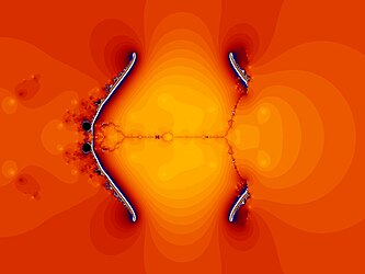  Mandelbrot set constructed from one point that is not a critical point; rendered without boundary and with jumps in the colouring
• 
  Mandelbrot set constructed using two different critical points; shows boundary in the upper half part and continuous colouring

The two images above show the opportunity for a more mathematically correct and more aesthetically pleasing way to render fractals than the method commonly used. The right hand image shows the boundary correctly and it does not exhibit the banding effects. Can this opportunity for improvement really be true? Can it be true, that twenty years after the Julia and Mandelbrot sets first saw the light of day, only now are technically perfect pictures beginning to turn up?

A possible explanation

The most influential book about Mandelbrot and Julia sets is probably Peitgen & Richter: The Beauty of Fractals from 1986. In this book you can see the first real pictures of the Mandelbrot set, because they were drawn by distance estimation and in black-and-white. Mandelbrot saw exciting patterns when he zoomed down into his set - stellate patterns of logarithmic spirals and uncanny and "hieroglyphical" reduced-size versions of the Julia sets - but he only see all this, because his maximum iteration number was low. The right hand picture below, with boundary and maximum iteration number 10,000 shows how the Mandlebrot set should look. The left picture is less mathematically precise, using 1,000 iterations, and is not calculating the boundary. If the left picture were drawn with the same maximum iteration number of 10,000, but still without the boundary calculation, we would only have seen the mini-mandelbrot visible in the centre of the right image. The other detail would be 'too fine' to see.

• 
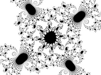  Without boundary calculation and with max iteration number 1,000
• 
  With boundary calculation and with max iteration number 10,000

Misconceptions from a Flawed Example Program

The Beauty of Fractals gives an almost correct computer program for the distance estimation shown in the right image. A possible reason that that method did not gain ground is that the procedure in this program is seriously flawed: The calculation of $z_{k}$ is performed (and completed) before the calculation of $z'_{k}$, and not after as it ought to be ($z'_{k+1}$ uses $z_{k}$, not $z_{k+1}$). For the successive calculation of $z'_{k}$, we must know $f'(z_{k})$ (which in this case is 2$z_{k}$). In order to avoid the calculation of $z_{k}$ (k = 0, 1, 2, ...) again, this sequence is saved in an array. Using this array, $z'_{k+1}=2z_{k}z'_{k}+1$ is calculated up to the last iteration number, and it is stated that overflow can occur. If overflow occurs the point is regarded as belonging to the boundary (the bail-out condition). If overflow does not occur, the calculation of the distance can be performed. Apart from it being untrue that overflow can occur, the method makes use of an unnecessary storing and repetition of the iteration, making it unnecessarily slower and less attractive. The following remark in the book is nor inviting either: "It turns out that the images depend very sensitively on the various choices" (bail-out radius, maximum iteration number, overflow, thickness of the boundary and blow-up factor). Is it this nonsense that has got people to lose all desire for using and generalizing the method?

References

Almost all the theorems and formulas in this Wikibook can be found in:

• Peitgen & Richter: The Beauty of Fractals, Springer-Verlag 1986 ISBN 0-387-15851-0.

See also these Wikipedia articles:

• Julia set
• Mandelbrot set
• Attractor

For the statement in the Postscript, see this article:

• The Sad Fate of the Fractals

Terminology

All the definitions are for points, functions, subsets, ... of the plane. We identify the points of the plane with the complex numbers and with vectors.

accumulation point (or cluster, or limit point) for a set: a point z such that each neighbourhood of z contains points of the set

boundary of a set: the set of points that are point of accumulation for the set as well as for the complement of the set

Cauchy-Riemann equations for a differentiable function $f(x,y)=f_{x}(x,y)+if_{y}(x,y)$ of the plane into itself: the two equations

${\frac {\partial }{\partial {x}}}f_{x}={\frac {\partial }{\partial {y}}}f_{y}$ and ${\frac {\partial }{\partial {y}}}f_{x}=-{\frac {\partial }{\partial {x}}}f_{y}$,

if they are satisfied, the function is differentiable as a complex function

cardioid: a heart-shaped curve (generated by a fixed point on a circle as it rolls round another circle of equal radius)

closed set: a set whose complement is an open set

complex number: a "two-dimensional" number, a number of the form (x, y), where x and y are real numbers, such a pair is usually written x+iy, where x and y are separated by the imaginary unit i, satisfying $i^{2}=-1$

convergence: a sequence $z_{i}$ (i = 0, 1, 2, ...) converges to the point z*, if for each neighbourhood U of z*, there exists a number N such that $z_{i}$ belongs to U for i > N. The sequence converges to the finite cycle C of order r, if for each point z* of the cycle the sequence $z_{n+ir}$ (for some n) converges to z*

countabel set: a set that can be put into a ono-to-one correspondance with the natural numbers, the rational numbers is a countabel set

critical point of a complex differentiable function f(z): a zero for the derivative f'(z)

cycle: a finite set of points in the plane, it can contain the point infinity, its number of elements is called its order

derivative (or differential quotient) of the complex function f(z) in the point z*: the number

$f'(z*)=(df(z)/dz)_{z=z*}=\lim _{h\to 0}(f(z*+h)-f(z*))/h$

(h complex) if it exists

determinant of the 2x2 matrix {$a_{ij}$}: the real number |{$a_{ij}$}| = $a_{11}a_{22}-a_{12}a_{21}$

holomorphic (or analytic) function: a complex function defined on an open set of the plane, that is complex differentiable in every point of the open set, such a function possesses derivatives of all orders

interior point of a set: a point z such that a neighbourhood of z is contained in the set

iteration: repeated operation with the same function f(z): $z_{1}=f(z_{0}),z_{2}=f(z_{1}),z_{3}=f(z_{2}),...$

lim: if the sequence $a_{n}$ (n = 0, 1, 2, ...) converges to the number a, we write lim_{n → ∞} a_n = a, if the value of the function f(z) converges to a for z converging to z*, we write lim_{n → ∞} f(z) = a

matrix: a rectangular array of numbers {$a_{ij}$} (i = 1, ..., m, j = 1, ..., n)

neighbourhood of a point z: a set containing a (small) circle with centre z

Newton iteration for an equation g(z) = 0: the iteration function $f(z)=z-g(z)/g'(z)$, if the sequence of iteration generated by a point converges to a fixed point, then this point is a solution to the equation g(z) = 0

norm of a complex number z = x+iy: the real number |z| = √(x² + y²) ≥ 0

open set a set all points of which are interior points

partial derivative with respect to x of the function f(z) in the point z: the number

$\partial f(z)/\partial {x}=lim_{h\to 0}(f(z+h)-f(z))/h$

where h is real (if it exists)

partial derivative with respect to y of the function f(z) in the point z: the number

$\partial f(z)/\partial {y}=lim_{h\to 0}(f(z+ih)-f(z))/h$

where h is real (if it exists)

polynomial of degree n: a function of the form $a_{0}+a_{1}z+a_{2}z^{2}+...+a_{n}z^{n}$

rational function: a function of the form p(z)/q(z), where p(z) and q(z) are polynomials

scalar product of the two vectors $v_{1}$ = {$x_{1}$, $y_{1}$} and $v_{2}$ = {$x_{2}$, $y_{2}$}: the real number $v_{1}*v_{2}=x_{1}x_{2}+y_{1}y_{2}=|v_{1}||v_{2}|cos(\theta )$, where $\theta$ is the angle between $v_{1}$ and $v_{2}$

transcendental function: a function that cannot be constructed in a finite number of steps from elementary functions and their inverses, e.g. $sin(z)=z-z^{3}/3!+z^{5}/5!-z^{7}/7!+...$, where n! = 1x2x3x...xn

uncountabel set: a set that is not countable, such a set (belonging to the plane) can be put into a one-to-one correspondance with the real numbers

Rules for operation with complex numbers

i² = -1

(x₁ + iy₁) + (x₂ + iy₂) = (x₁ + x₂) + i(y₁ + y₂)

(x₁ + iy₁)(x₂ + iy₂) = (x₁x₂ - y₁y₂) + i(x₁y₂ + x₂y₁)

(x₁ + iy₁)/(x₂ + iy₂) = ((x₁x₂ + y₁y₂) + i(-x₁y₂ + x₂y₁))/ (x₂² + y₂²)

The conjugate number to $z=x+iy$ is $z^{-}=x-iy$, that is, the reflection of z in the x-axis. The norm of z is the real number |z| = √(x² + y²). We have $|z|^{2}=zz^{-}$. From this, we can derive the rule for division: $z/w=zw^{-}/(ww^{-})=zw^{-}/|w|^{2}$.

A complex number z = x + iy can be written

$z=r(sin(\theta )+icos(\theta ))$

where r is the norm of z:

r = |z| = √(x² + y²)

and where the angle $\theta$ is the argument arg(z) of z:

$\theta$ = arctan(y/x) for x > 0

$\theta$ = arctan(y/x) + $\pi$ for x < 0

arg(z) is multivalued: arg(z) = $\theta +n2\pi i$, for every integer n.

The point $sin(\theta )+icos(\theta )$ (lying on the unit circle) is also denoted $e^{i\theta }$, and we define the exponential function $exp(z)$ by

$exp(z)=e^{z}=e^{x+iy}=e^{x}e^{iy}$

The sinus and cosinus relations can be written

$cos(\theta _{1}+\theta _{2})+isin(\theta _{1}+\theta _{2})=(cos\theta _{1}+isin\theta _{1})(cos\theta _{2}+isin\theta _{2})$

and from this we see that $e^{z}$ has the exponential property for z imaginary:

$e^{i(\theta _{1}+\theta _{2})}=e^{i\theta _{1}}e^{i\theta _{2}}$

The logarithm function log(z) is defined as the inverse function to exp(z): log(z) = w if exp(w) = z. We have log(z) = log|z| + i arg(z). log(z) is multivalued: $log(z)=w+n2\pi i$, for every integer n.

For a positive real number a and a complex number z, we define $a^{z}=e^{log(a)z}$. For a complex number z, the power $z^{n}$ is only defined when the exponent n is an integer.

Differentiable complex function

A complex function defined on an open domain of the plane is called holomorphic (or analytic), if it is differentiable in every point of this domain. If that is so, the derived function f'(z) is also differentiable in every point (this theorem is not true for real functions). We have the usual rules for differentation:

$d(f(z)+g(z))/dz=df(z)/dz+dg(z)/dz$

$d(f(z)g(z))/dz=(df(z)/dz)g(z)+f(z)(dg(z)/dz)$

$(d(f(g(z))/dz)_{z*}=(df(z)/dz)_{g(z*)}(dg(z)/dz)_{z*}$

$dz^{n}/dz=nz^{n-1}$ (n integer)

$da^{z}/dz=log(a)a^{z}$ (a positive real number)

$d(exp(z))/dz=exp(z)$

$d(log(z))/dz=1/z$

From these rules, we can derive all we need, for instance:

$d(f(z)^{-1})/dz=-f'(z)/f(z)^{2}$

$d(log(f(z)))/dz=f'(z)/f(z)$

For the computer it is easy to find f'(z): f'(z) = (f(z+h) - f(z))/h for $h=10^{-9}$, for instance.

The derivative of a function into the real numbers

The real function f(z) on a domain of the plane, is differentiable in the point z, if

lim_{t → 0} (f(z + th) - f(z))/t

(t real) exists for every complex number h, and if the hereby defined function $Df(z)(h)$ from the complex numbers (h) into the real numbers satisfies $Df(z)(h_{1}+h_{2})=Df(z)(h_{1})+Df(z)(h_{2})$. As we also have $Df(z)(th)=tDf(z)(h)$, for t real, this mapping is linear. It is called the derivative of f(z) in the point z.

The linearity means that $Df(z)$ is determined by the two real numbers $Df(z)(1)$ and $Df(z)(i)$. These are denoted by ∂f(z)/∂x and ∂f(z)/∂y, respectively, and are called the partial derivatives with respect x and y. We have for $h=h_{x}+ih_{y}$:

Df(z)(h_x + ih_y) = (∂f(z)/∂x)h_x + (∂f(z)/∂y)h_y

This number is the scalar product of the vectors (∂f(z)/∂x, ∂f(z)/∂y) and ($h_{x},h_{y}$), so, if we regard Df(z) and h as vectors, we can write:

Df(z)(h) = Df(z)*h.

The vector Df(z) is called the gradient of f(z) in the point z: the direction of Df(z) is the direction of the most rapid growth and the length of Df(z) is the growth of f(z) in this direction.

If ∂f(z)/∂x and ∂f(z)/∂y exist in a neighbourhood of z* and are continuous in z*, then f(z) is differentiable in z*.

The derivative of a mapping into the plane

If f(z) is a mapping from a domain of the plane into the plane, we can write $f(z)=f_{x}(z)+if_{y}(z)$, where $f_{x}(z)$ and $f_{y}(z)$ are real functions. f(z) is called differentiable in the point z (as real function), if both $f_{x}(z)$ and $f_{y}(z)$ are differentiable in z. If that is so, we have a linear mapping Df(z) from the complex plane into itself given by $Df(z)(h)=Df_{x}(z)(h)+iDf_{y}(z)(h)$. This linear mapping is called the derivative of f(z) in the point z.

The linearity means that Df(z) is determined by the two complex numbers Df(z)(1) (= ∂f_x/∂x + i∂f_y/∂x) and Df(z)(i) (= ∂f_x/∂y + i∂f_y/∂y), and we have:

Df(h_x + ih_y) = ((∂f_x/∂x)h_x + (∂f_x/∂y)h_y) + i((∂f_y/∂x)h_x + (∂f_y/∂y)h_y)

In matrix notation, this means that Df(z) is the linear mapping from the plane into itself given by

${\begin{bmatrix}\partial f_{x}/\partial {x}&\partial f_{x}/\partial {y}\\\partial f_{y}/\partial {x}&\partial f_{y}/\partial {y}\\\end{bmatrix}}\times {\begin{bmatrix}h_{x}\\h_{y}\\\end{bmatrix}}$

That f(z) is differentiable as a complex function, means that this multiplication corresponds to multiplication by the complex number f'(z), and this is the case precisely when the Cauchy-Riemann equations

${\frac {\partial }{\partial {x}}}f_{x}={\frac {\partial }{\partial {y}}}f_{y}$ and ${\frac {\partial }{\partial {y}}}f_{x}=-{\frac {\partial }{\partial {x}}}f_{y}$

are satisfied - these two number are the real and the imaginary part of f'(z).

Matrix calculus

A matrix is a rectangular array of real numbers. We will only need matrices of side 1 or 2. That is, either a 2x2-matrix (quadratic matrix):

${\begin{bmatrix}a&b\\c&d\\\end{bmatrix}}$

or a 1x2-matrix (a row-matrix): {a, b}, or a 2x1-matrix (a column-matrix):

${\begin{bmatrix}a\\b\\\end{bmatrix}}$

or a 1x1-matrix: {a}, identified with the number a.

The transpose of a matrix, is the matrix formed by reflection in the diagonal. This operation is denoted by *, and it means that we can denote a column-matrix by {a, b}* - the transpose of the row-matrix {a, b}.

Two matrices A and B of the same type can be added by adding the number on the corresponding places. We multiply a matrix by a real number by multiplying each of its elements by this number.

Two matrices A og B, where the width of A is equal to the height of B can be multiplied: the result is a matrix AB whose height is the height of A and whose width is the width of B:

${\begin{bmatrix}a&b\\c&d\\\end{bmatrix}}\times {\begin{bmatrix}\alpha &\beta \\\gamma &\delta \\\end{bmatrix}}={\begin{bmatrix}a\alpha +b\gamma &a\beta +b\delta \\c\alpha +d\gamma &c\beta +d\delta \\\end{bmatrix}}$

${\begin{bmatrix}a&b\\c&d\\\end{bmatrix}}\times {\begin{bmatrix}\alpha \\\beta \\\end{bmatrix}}={\begin{bmatrix}a\alpha +b\beta \\c\alpha +d\beta \\\end{bmatrix}}$

The product {a, b}{$\alpha ,\beta$}* is the number $a\alpha +b\beta$ (the scalar product of the vectors {a, b} and {$\alpha ,\beta$}) and the product {a, b}*{$\alpha ,\beta$} is the 2x2-matrix

${\begin{bmatrix}a\alpha &a\beta \\b\alpha &b\beta \\\end{bmatrix}}$

The determinant of the quadratic matrix A =

${\begin{bmatrix}a&b\\c&d\\\end{bmatrix}}$

is the real number det(A) = |A| = ad - bc. The unit-matrix I is

${\begin{bmatrix}1&0\\0&1\\\end{bmatrix}}$

The inverse matrix to the 2x2-matrix A, is the 2x2-matrix $A^{-1}$ satisfying $AA^{-1}=A^{-1}A=I$. It is given by:

${\begin{bmatrix}d&-b\\-c&a\\\end{bmatrix}}$

divided by |A| - it does therefore only exist for |A| <> 0.

The points of the plane can be identified with the column matrices {x, y}*. Therefore, a 2x2-matrix A determines a linear mapping of the plane into itself: {x, y}* → A{x, y}*. It is injective (and then also bijective) if |A| <> 0. If that is so, the number |A| is the area of the image of the unit-square (if |A| is negative, the mapping changes orientation). Likewise, the vectors of the plane can be identified with the row-matrices {a, b}. A row-matrix {a, b} determines a linear mapping of the plane into the real numbers: {x, y}* → {a, b}{x, y}* = ax + by (the scalar product of the vectors {a, b} and {x, y}). The complex number z = x + iy can be identified with the column-matrix {x, y}* and with the 2x2-matrix

${\begin{bmatrix}x&-y\\y&x\\\end{bmatrix}}$

The mapping of the plane into itself given by this matrix, is the multiplication by the complex number z.

Computer programs

We will show two ways of making a program that can draw a Mandelbrot set where the iterations are towards ∞: a program where all is done from the ground, but which does nothing more than drawing a single picture, and a program where you can do all you desire (zoom, alter colouring and render as file), but where these facilities are handed over to another program, namely Ultra Fractal.

A single picture

Section of the Mandelbrot set for $z^{2}+0.009/z+c$

Let us make a program that is as simple as possible: it draws a single picture, and does nothing more (when it has done its work it closes). It was originally written in assembly language, but here we write it in pseudo-code. It consists of two parts: the drawing procedure and the colour scale.

We draw a section of the Mandelbrot set for the family $f(z)=z^{2}+{\frac {p}{z}}+c\,$, for p = 0.009. We let the size of the window be 800x600 pixels, and we imagine that the section has its lower left corner in the point with coordinates (ax, ay) and that is has width h. We have $f'(z)=2z-{\frac {p}{z^{2}}}\,$, so that the finite critical point we need, is solution to the equation $z^{3}=p/2$. We choose the real solution cri = $(p/2)^{1/3}$.

The drawing procedure

p = 0.009

cri = $(p/2)^{1/3}$

r = 1.0E200 (square of the bail-out radius)

u = log(log(r))

v = 1/log(2) (2 is the degree of the rational function)

ax = -0.7028233689263 (x-coordinate of lower left corner)

ay = 0.1142331238418 (y-coordinate of lower left corner)

h = 0.0092906805859 (width of the section)

g = h / 800

m = 850 (maximum iteration number)

thick = h * 0.0005 (thickness of the boundary)

dens = 24.9 (density of the colours)

disp = 432.0 (displacement of the colour scale)

for i = 0 to 799 do

begin

cx = ax + i * g (x-coordinate of pixel (i, j))

for j = 0 to 599 do

begin

cy = ay + j * g (y-coordinate of pixel (i, j))

x = cri

y = 0

xd = 0

yd = 0

f = 0

n = 0

while (n < m) and (f < r) do

begin

n = n + 1

x1 = x * x - y * y

y1 = 2 * x * y

f = x * x + y * y

x2 = 2 * x - p * x1 / (f * f)

y2 = 2 * y + p * y1 / (f * f)

temp = xd

xd = x2 * xd - y2 * yd + 1

yd = x2 * yd + y2 * temp

fd = xd * xd + yd * yd

x = x1 + p * x / f + cx

y = y1 - p * y / f + cy

f = x * x + y * y

end

if (n = m) or (log(f) * sqrt(f) < thick * sqrt(fd)) then

setpixel(i, 599 - j, 0)

else

begin

s = n - v * (log(log(f)) - u)

n = round(dens * s + disp) mod 720

col = paletteRGB(col1[n], col2[n], col3[n])

setpixel(i, 599 - j, col)

end

end

end

Explanation

We have set $c=cx+icy$, $z=x+iy$, $z'=xd+iyd$ and $x1+iy1=(x+iy)^{2}$, and we have used that $1/z=z^{-}/|z|^{2}$.

The successive calculation of the derivative z' is $xd+iyd=(x2+iy2)*(xd+iyd)+1$, where $x2+iy2=2*(x+iy)-p*(x1-iy1)/(f*f)$ and $f=x^{2}+y^{2}$. The next point in the iteration is $x+iy=(x1+iy1)+p*(x-iy)/f+(cx+icy)$. The distance function is

log(√f)*√f/√fd   (= log(f)*√f/(2*√fd))

for the last z-value, here $f=x^{2}+y^{2}$ and $fd=xd^{2}+yd^{2}$. The number in the interval [0, 1[ to be subtracted from the iteration number (in order to get the real iteration number), is $log(log(|z|)/log(r))/log(2)=v*(log(log(f))-u)$, for the last z, here $v=1/log(2)$ and $u=log(log(r))$.

paletteRGB(r, g, b) is the integer indexing the colour with RGB-values (r, g, b), 0 gives black. col, col2 and col3 are the arrays from 0 to 719 of integers from 0 to 255 constructed in the next section.

The colour scale

A colour is immediately (in the computer) given by its composition of the three primary colours red, green and blue, and their shares are measured in whole numbers between 0 and 255. This triple of numbers is the set of RGB values of the colour. The colours correspond accordingly to the entire points in a cube with side length 256, and we construct our cyclic colour scala by going regularly along an ellipse in this cube. An ellipse in the space is determined by:

a centre with coordinates (a, b, c)

a major axe rmaj and a minor axe rmin

two angles angle g and h determining the direction of the plane of the ellipse

an angle q determining the direction of the ellipse in this plane

u = cos(g * pi / 180) * cos(h * pi / 180) {(u,v,w) is a unit vector orthogonal to the plane}

v = cos(g * pi / 180) * sin(h * pi / 180)

w = sin(g * pi / 180)

x = -a {(x,y,z) is a vector in the plane}

y = -b

z = a * u / w + b * v / w

e = sqrt(sqr(x) + sqr(y) + sqr(z))

x1 = x / e {the unit vector corresponding to (x,y,z)}

y1 = y / e

z1 = z / e

x2 = v * z1 - w * y1 {the unit vector in the plane orthogonal to (x1,y1,z1)}

y2 = w * x1 - u * z1

z2 = u * y1 - v * x1

e = cos(q * pi / 180)

f = sin(q * pi / 180)

x1 = e * x1 + f * x2 {the unit vector in the plane in the direction of the angle q}

y1 = e * y1 + f * y2

z1 = e * z1 + f * z2

x2 = v * z1 - w * y1 {the unit vector in the plane orthogonal to this direction}

y2 = w * x1 - u * z1

z2 = u * y1 - v * x1

for i = 0 to 719 do

begin

e = rmaj * cos(i * pi / 360)

f = rmin * sin(i * pi / 360)

col1[i] = round(a + e * x1 + f * x2) {the three coordinates of the point on the ellipse}

col2[i] = round(b + e * y1 + f * y2)

col3[i] = round(c + e * z1 + f * z2)

end

In the picture we have: (a, b, c) = (176, 176, 176), rmaj = rmin = 88, g = 146, h = -32, q = 0.

Ultra Fractal

Ultra Fractal is a program for drawing fractals where the user to a great extent can write his own formula programs and where the main program performs all that is common for all the fractal procedures, that is, the procedure of going from pixel to pixel, zooming, colouring, production of a large picture as a file. Your effort is reduced to a minimum, and apart from pictures that cannot be drawn regularly from pixel to pixel - attractors and landscapes, for instance - you can do all you desire: non-complex functions, quaternions, ... You can operate directly with complex numbers.

First you should download a free trial-version of the program and learn how it works. Then you should see the article Make attractive pictures of Mandelbrot and Julia sets with Ultra Fractal, and download the (free) programs from this site to be run with Ultra Fractal.

For the drawing two programs have to be combined: a formula program and a colouring program. In the formula program is a section called loop, and when this loop has done its work, the number of iterations and the last value of the complex number z are transferred to the colouring program, which calculates the colour from these two numbers. However, Ultra fractal is designed to "all" types of fractals, and unfortunately the Julia and Mandelbrot sets do not quite fit into this form: for iterations towards cycles, the iteration has to be continued in order to find the order and the attraction of the cycle, and it is not the last value of z in the sequence we do use for the colour. Therefore we replace this loop by a fictive loop (which only runs one time) and perform all the operations in the section init. This implies that we cannot use the default colouring program of Ultra Fractal, we must write a new colouring program.

Another thing you must be aware of, is that in Ultra Fractal the norm |z| of the complex number z is the square of its length: |z| = $x^{2}+y^{2}$.

Section of the Mandelbrot set for $z^{2}/2+0.26*z^{4}+c$

We will show a program that draws the Mandelbrot set for the family $f(z)+c$, where $f(z)$ is a polynomial whose first two terms are zero, so that it begins with $z^{2}$ or a larger power of z, because we then can take 0 as the finite critical point.

The two programs can be copied and inserted in an empty formula and colouring document, respectively. We have inserted the polynomial $z^{2}/2+p*z^{4}+c$ of degree 4, where p is a real parameter. The picture shows a section of the Mandelbrot set for p = 0.26.

The formula program

Mandelbrot {

global:

float p = 0.26 ;parameter

float deg = 4 ;degree of the polynomial

float v = 1 / log(deg)

float g = 10 * log(10)

float r = exp(g) ;square of the radius of the bail-out circle

float u = log(g)

float tb = sqr(@thick / (1000 * #magn)) ;for the thickness of the boundary

float h = 1 / (1500 * #magn * @width) ;a very small real number

init:

complex z = 0 ;critical point

complex zd = 0 ;the sequence of the derivatives

complex z1 = 0

float w = 0

int n = 0

while n < #maxit && |z| < r

n = n + 1

z1 = z^2/2 + p*z^4

zd = ((z+h)^2/2 + p*(z+h)^4 - z1) * zd / h + 1

z = z1 + #pixel

endwhile

if n == #maxit || sqr(log(|z|)) * |z| < tb * |zd|

w = -1

else

w = n - v * (log(log(|z|)) - u)

endif

;begin fictive loop

z = 0

n = 0

loop:

n = n + 1

z = z + #pixel

if n == 1

z = w

endif

bailout:

n < 1

;end fictive loop

default:

title = "Mandelbrot"

maxiter = 100

param thick

caption = "boundary"

default = 1.0

endparam

param width

caption = "width"

default = 640

endparam

}

Explanation

We have set the square of the radius r of the bail-out circle to $10^{10}$, and set the thickness of the boundary to "thick/(1000 * #magn)", so that it becomes thinner when we zoom in.

We have calculated the derivative $f(z)$ by $(f(z+h)-f(z))/h$ for a small number h, namely "h = 1/(1500*#magn*width)", where "width" is the width of the picture. The default value is the width of the window in pixels (here set to 640), but if you draw a large picture, you should enter the width of this.

The successive calculation of the derivative $z'_{k+1}=f'(z_{k})z'_{k}+1$ is "zd = (f(z+h) - f(z)) * zd / h + 1". The next iteration $z_{k+1}=f(z_{k})+c$ is "z = f(z) + #pixel". The square of the distance estimation $log|z_{k}|*|z_{k}|/|z'_{k}|$ is "sqr(log(|z|)) * |z| / |zd|". The number to be subtracted from the iteration number $log(log(|z_{k}|)/log(r))/log(deg)$ is "v * (log(log(|z|)) - u)", where "v = 1/log(deg)" and "u = log(log(r))".

The final complex number z (to be transferred to the colouring program), which here actually is real, is set to -1, when the point belongs to the Mandelbrot set or to the boundary, otherwise it is set to the real iteration number. It is transferred to the colouring program, which we have called Gradient, as #z, and is here set equal to the real number s. When s is negative the colour is set to "#solid", otherwise we multiply s by a number "dens" determining the density, and add to this number a number "disp" determining the displacement of the scale, and as we want this displacement to be a per cent, we divide the result by 100: "u = (dens * s + disp) / 100". In Ultra Fractal the colours of the cyclic colour scales are indexed by the real numbers in the interval [0, 1[, and we let this number, "#index", be the non-integral part of the number u: "#index = u - trunc(u)".

The colouring program

Gradient {

final:

float s = real(#z)

float u = 0

if s < 0

#solid = true

else

u = (@dens * s + @disp) / 100

#index = u - trunc(u)

endif

default:

title = "Gradient"

param disp

caption = "displace"

default = 0

endparam

param dens

caption = "density"

default = 1.0

endparam

}

Favourite formulas

If you insert a random complex rational function in a fractal program, it is very unlikely that you will find an interesting locality in the Mandelbrot set. But sometimes you will witness a startling spectacle when you zoom in. And this is usually where two domains of different structures meet each other.

If you come across an interesting formula, then let the rest of us see it. You can here write the formula and the coordinates of the locality, and show a picture. You should also state the critical points, however you can neglect this, if you use ∞ and a real point of smallest numerical value, or if you (in case of iterations towards finite cycles) use two conjugate complex numbers of largest distance.

You should fell free to remove formulas that clearly have been surpassed by others.

$z^{2}/2+z^{4}/4+c$ c = (0.7, 1.3)

$1-z^{2}+z^{5}/(2+4z)+c$ c = (-0.163, 0.085)

• 
  The Mandelbrot set for $z^{2}/2+z^{4}/4+c$
• 
  The Mandelbrot set for $1-z^{2}+z^{5}/(2+4z)+c$

References

- ↑ Boundary set renderings, juliasets.dk (started 2003 and completed 2009)