Foreword

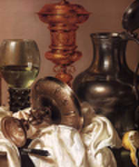
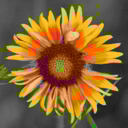
Drawing perfect but file compressed too much
File perfect but drawing incomplete

When the era of digital pictures began, a serious problem arose:

A digital picture took up a great deal of storage space.

At that time computer memory was more expensive than it is now. The memory requirements were a very significant problem. Moreover, the electronic transmission of data was slow. A method had to be found by which the data could be compressed. The compression method could lose some information. It could be acceptable to introduce small changes in colour values if the overall impression of the picture were preserved. Sadly the solution to this problem is not, as one might hope, a nice piece of mathematical work in the classical sense. It involves experiments with the ability of the human eye to discern colour nuances compared with light intensity. Strange tables appear in the procedure.

The JPEG method was a result of collaboration. JPEG stands for "Joint Photographic Expert Group". The expert group was organized in 1986 and in 1992 issued a standard for their new image file format, JPEG. Since that time this format has been the most commonly used format for storing and transmitting photos.

The JPEG method is not difficult to understand. However, it is difficult to acquire knowledge about the method, mainly because it is not a fixed and final procedure but rather a principle. The number of articles that try to explain the method is immense. They often contain misunderstandings strongly suggesting the author himself has not made, or closely studied, a program that can produce a file or draw the picture from a file.

Hence this Wiki book.

Parts One and Two

This Wiki book is divided into two parts. Each is accompanied by programs. These are closely described and used to make illustrations and experiments.

Part one explains the idea. We have altered the method a little so that it is easier to understand. Our alterations allow us to introduce variables in order to make interesting experiments. Our method is rather simple. Naturally, it does not compress as efficiently as the real JPEG method, but it is still surprisingly good. It can compress a file so that the data take up about 7 per cent of the original data of the picture. When you have read part one, you will have a good understanding of the principle of the JPEG method. If it was merely this you were looking for, you will not become very much wiser by reading part two.

Part two is based on two articles:

The official document (from 1992) where the method is described in full and recommended as international standard;
The document (also from 1992) specifying the standard for the implementation of the method which has become the most commonly used - almost all JPEG pictures you will meet are in accordance with this implementation.

We explain all the things necessary for making a program that can produce efficiently compressed JPEG files. We provide a program that can draw the pictures of the most commonly used JPEG file types. We have also made a program that can show all the most relevant information in the header part of a JPEG file. Some experience with this program can help you to understand the arrangement of a JPEG file. You can use this information (copy it or use it as guidelines), if you want to make your own JPEG compressor - for instance as a component of a program that can make computer graphics.

About the Pictures

All the pictures in this book were made with the program in part two - also those in part one, since the files made with the demonstration program are not true JPEG files.

The colour components

The BMP format

In the computer a colour is given by its composition of the three primary colours red, green and blue, and their shares are measured in bytes, that is, integers from 0 to 255. Therefore a colour corresponds to a triple of bytes, called a RGB triple. A picture is a rectangular matrix of RGB triples. If the picture is of width w and height h, the colour values (RGB triples) are indexed by the pairs (i, j), i = 0, ..., w-1, j = 0, ..., h-1, so that the left top corner has coordinate set (0, 0)(that is, the ordinate is measured downwards). The picture takes up 3wh bytes, and it can be stored in a memory-block by storing the h horizontal lines consisting of 3w bytes one after another. The procedure for showing the picture by transferring the memory-block (directly) to the screen is called a bitmap.

(In the bitmap procedure of Windows it is demanded that the number of bytes in the horizontal lines is divisible by 4, this means that the line segments of the memory-block possibly must be increased by 1, 2 or 3 bytes, usually filled with zeros.)

A picture can be stored permanently in a file consisting of the data bytes arranged in this way and supplied with a header specifying the type of the file and the dimensions of the picture. This is so for the BMP file format of Windows (BMP = Bit Map Picture). A BMP file begins with a header of 54 bytes. As the data in a BMP file lie precisely in the way used to draw a bitmap, the picture can be drawn directly from the reading of the file - without involving RAM-memory and without the use of other than elementary arithmetic calculations.

(The header of a BMP file is divided up in 17 blocks consisting of one, two or four bytes. Two bytes determine an integer from 0 to 256² - 1 = 65535, called a word, and four bytes determine an integer from 0 to 256⁴ - 1 = 4294967295, called a double word. The first two blocks of the BMP header are the bytes 66 and 77, identified with the characters 'B' and 'M' and specifying the type of the file. Block 8 and 9 are double words stating the width and the height, block 10 and 11 are words, usually set to 1 and 24 (= bit per colour), respectively, and block 7 is a double word usually set to 40. The other blocks, except block 4 and 5, which are words, are double words, and all these blocks can be set to 0, as they usually are not read by the program reading the file.)

Data compression

The BMP file format and a memory-block to be transferred to the screen as a bitmap are easy tasks for the computer and for the programmer, but these ways of storing a picture take up a lot of memory: a picture of 1000x750 pixels takes up 3x1000x750 = 2.2 Mb. This can be accepted provisionally in the working-up procedure of a picture or for storing of relatively few pictures where the highest possible quality is desired, but so much space is unacceptable in folders with hundreds of pictures or in films or in transmissions from the internet. One would immediately think that it is impossible to get digitalized data to take up lesser space, because the material with the bits cannot be reduced like a photographic negative. But a digitalized data set consists of sequences of bits, and these can be replaced by sequences that are shorter - and if there are repetitions, the thing that repeats itself can be replaced by a sequence which acts as a symbol for its type and the number of repetitions. If the data are copies of the elements in some fixed set (of numbers, for instance), then we can assign to the elements of the set sequences of bits such that the elements which are used most frequently are assigned to the shortest sequences. Besides, if the elements of the data set are numbers of strongly varying size, we can, instead of allocating equal space to each number, try to remove the empty spaces between the numbers. This cannot of course be done without ceremony, since (in lack of a third bit) we must have a tool with which we can separate the sequences of bits corresponding to the numbers. However, we can insert sequences of bits acting as codes.

Only a non-negative integer can immediately be digitalized, namely by writing its binary digit expression:

n = c_m2^m + ... + c₂2² + c₁2 + c₀

where c₀, ..., c_m are bits: 0 or 1 - we order the sequence so that the most significant bit comes first. If the number is rational or real, we must in some way express it as the composite of two non-negative integers. The codes to be inserted can be chosen so that they are in one-to-one correspondence with the natural numbers, and such that the natural number assigned to a code is the number of digits of the following non-negative integer. The codes must be chosen so that the most frequently used natural numbers (stating number of digits) have the shortest codes, and moreover so that we can determine when a code ends.

When the data are to be used (in order to show a picture, for instance), the compressed data set is subjected to a decoding procedure, leaving a data set that is exactly as the original. In almost all image file formats there is a possibility for compressing the data in this way. Such tricks are of course used in the JPEG procedure, but in this procedure the data are modified before the compression: by first transforming the colour values and then reducing the new values by dividing them by certain numbers and rounding off. The last procedure is called quantization and it may introduce (small) deviations.

The RGB values

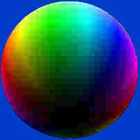
The basis colours are the pure colours, these are the "strongest" colours which have maximum saturation. The pure colours make up a cyclic colour scale:

The pure colours

Therefore a pure colour is determined by an angle. Every colour different from a grey scale colour is the result of mixing a uniquely determined pure colour with a grey scale colour. The pure colours are not of the same luminance: three of them have lesser luminance than the others, and these are the primary colours: pure red, pure green and pure blue, assigned to the angles 0, 120 and -120 degrees. A pure colour that is not primary lies between two primary colours, and is the result of mixing the nearest of these with part of the other. If we mix the three primary colours, we get white - the colour of maximum luminance. From this we can see that every colour is produced by mixing the three primary colours, each made more or less darker. This is the RGB representation. We usually measure the three amounts in bytes, so that 255 corresponds to the primary colour and 0 corresponds to black.

(We can find the pure colour associated to the colour C (different from a grey scale colour) in the following way: By subtracting the RGB values of C from white, we get the colour C1 with RGB triple (255-R, 255-G, 255-B). If we assume that blue has most share in this colour, then C1 = β C2, for some β <= 1 and a colour C2 for which blue has share 255. By subtracting C2 from white, we get a colour C3, and if we assume that red has most share in this, then C3 = α C4, for some α <= 1 and a pure colour C4, for which red has share 255 and blue has share 0. This is the pure colour associated to C, and we get C by mixing this pure colour with black according to α and with white according to β.)

The YCbCr values

There is, however, a drawback to the RGB representation of the colours: the three values are of equal significance. We would prefer a triple representation where one of the values (the first) was more significant than the two others, because then, in the quantization procedure, we could allow larger deviations in the two less significant components. Such a representation is easy to imagine, as the four pictures below show: we can let the first value in the triple be the average value of the three RGB values, thus expressing the intensity of the colour (and giving the corresponding grey scale picture), and let the two other values form the "colour additions". We imagine the colours (the RGB triples) as the integral points in a cube of side length 256, having the three positive coordinate axes as sides, and its origin in the corner corresponding to black. In this cube the grey scales lie on the diagonal, and we take the diagonal as the first axis. We could let the two other coordinate axes be orthogonal to the diagonal and to each other, but in order to get a simple transform, we let them lie in the B-G-plane and the R-G-plane. Note that the new coordinate system means the two last colour values can be negative. We choose the units such that the first coordinate is measured in bytes and the two others are measured in signed bytes: integers from -128 to 127. The new coordinate triple is connected with the RGB triple by a linear transform.

We call the new representation the YCbCr values of the colour. Y stands for luminance (or luma) and C stands for chroma: Cb for chromatic blue and Cr for chromatic red. Our assumptions mean that there are parameters kb and kr, such that the linear transform and its inverse are given by:

Y = kr∙R + (1 - kr - kb)∙G + kb∙B

Cb = ½(B - Y)/(1 - kb)

Cr = ½(R - Y)/(1 - kr)

R = Y + 2(1 - kr)∙Cr

G = Y - (kb∙(B - Y) + kr∙(R - Y))/(1 - kb - kr)

B = Y + 2(1 - kb)∙Cb

We see that if a colour is a grey scale colour, that is, if R = G = B, then Y is this number and Cb and Cr are zero. Mathematically, it would be natural to set kb and kr to 1/4, because the transform then would get a simple and natural form:

Y = R/4 + G/2 + B/4

Cb = -R/6 - G/3 + B/2

Cr = R/2 - G/3 - B/6

R = Y + (3/2)Cr

G = Y - (3/2)(Cb + Cr)/2

B = Y + (3/2)Cb

However, in the JPEG implementation - which we are guided by here - the parameters kb and kr are set to 0.144 and 0.299, and with these values the formulas become:

Y = 0.299∙R + 0.587∙G + 0.114∙B

Cb = -0.168736∙R - 0.331264∙G + 0.5∙B

Cr = 0.5∙R - 0.418688∙G - 0.081312∙B

R = Y + 1.402∙Cr

G = Y - 0.3441∙Cb - 0.71414∙Cr

B = Y + 1.772∙Cb

This means that the coordinate axes are: the diagonal, the line (-0.34, 1.77) in the G-B-plane and the line (1.40, -0.71) in the R-G-plane. As the two chromatic coordinates range in the interval [-128, 127], we must add 128 to them in order to get bytes, so that we can draw "projections" of the picture on the coordinate axes. Instead of the composition of the picture in pictures in red-, green- and blue-scales, we now get pictures in grey-scale, blue-green-scale and red-green-scale:

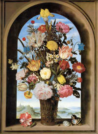The original picture
The grey scale component

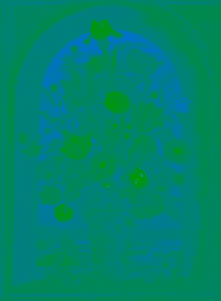The blue-green component
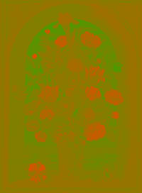The red-green component

As we want our numbers (integers) numerically as small as possible, we subtract 128 from the Y value, so that this, like the Cb and Cr, becomes a signed byte.

The transform and quantization

The cosine transform

With the YCbCr representation of the colours, we can say that the picture is composed of three pictures of which the first is more significant than the two others. These three pictures are called the components of the picture: the Y component, the Cb component and the Cr component. But we can continue this process of getting few important and more less important elements. Let us assume that we have a picture in grey scale, then we can imagine that we start with a picture of only one colour, namely the average colour of all the colours in the picture, and by additions introduce more and more variation in the picture, so that at the end we have the complete picture. Then it would possibly turn out, that we could omit some of the last operations, as we were not able to distinguish the new additions. However, the expansion (which we have in mind) of the colour function in a sequence of terms having smaller and smaller importance, works only for a quadratic picture. Therefore our picture must be divided up in squares. And these squares must be rather small, because the number of calculations grows with the fourth power of the side length of the squares, which means that if the small squares are made twice as large, the number of calculations becomes four times as large. On the other hand, if the small squares are too small, the effect of the procedure is diminished. The optimal side length of the small squares seems to be 8-12 pixels. In JPEG the picture is divided up in 8x8-squares, but here we will see what happens if we let the squares have another side length than 8: we have arranged the program so that we can choose one of the numbers 2, 3, ..., 24 as side length s.

Thus, we perform a regular dividing up of the picture in sxs-squares. In JPEG this is done by starting at the left top corner and going from left to right line-wise from top to bottom, just as when we read a text. In our program for demonstration of the theory, we will however go through the picture in another way, namely column-wise from left to right and zigzagging down and up, so that the squares continually have a side in common. We will assume that the width and the height of the picture are divisible by s, or rather: we will only use the part of the picture lying within the largest domain (starting at the left top corner) which can be divided regularily up in sxs-squares. The method we use to expand the colour function within a square, is the discrete cosine transform (DCT) defined as follows.

We assume that we have a quadratic picture (in grey scales) of side length N, and we assume that N is rather large, so that we can talk about a "real" picture. This picture is a NxN-matrix of colour values (bytes): f(i, j), i, j = 0, 1, ..., N-1 (remember that (0, 0) corresponds to the left top corner, so that the ordinate j is measured downwards). We want to express f(i, j) in terms of pure double oscillations of the form f_{u, v}(i, j) = c(i, u) ∙ c(j, v), u, v = 0, ..., N-1, where the function c(i, u) is given by:

c(i,u)=\cos {\frac {(2i+1)u\pi }{2N}}

Note that f_{0, 0}(i, j) is constant 1 and that the function f_{u, v}(i, j) oscillates more the larger u or v are. We therefore want to express f(i, j) as a double sum of N² terms:

f(i,j)=\sum _{u=0}^{N-1}\sum _{v=0}^{N-1}h(u,v)\cdot c(i,u)\cdot c(j,v)

where the h(u, v)'s are (real) coefficients. The first term (u = 0 and v = 0) being a constant function is the average value of the N² numbers f(i, j). The following terms oscillate more and more (as functions of i and j), and if we omit some of the last terms, we get an approximation to f(i, j) that is free from the largest frequencies.

We can find the coefficients h(u, v) of this series expression of f(i, j) in the following way. Let the NxN-matrix (of real numbers) g(u, v) (u, v = 0, 1, ..., N-1) be defined by:

g(u,v)={\frac {2\lambda (u)\lambda (v)}{N}}\sum _{i=0}^{N-1}\sum _{j=0}^{N-1}c(i,u)\cdot c(j,v)\cdot f(i,j)

where λ(u) is 1 for u ≠ 0 and 1/√2 for u = 0. The matrix g(u, v) is called the (forward) discrete cosine transform (DCT or FDCT) of the matrix f(i, j). Note that g(0, 0) = N times the average of the colour values. There is a formula which, from the NxN-matrix g(u, v), brings us back to the original NxN-matrix f(i, j), and it has an analogue look:

f(i, j) = (2/N)∑_{u, v = 0, ..., N-1}λ(u)λ(v) ∙ c(i, u) ∙ c(j, v) ∙ g(u, v)

f(i,j)={\frac {N}{2}}\sum _{u=0}^{N-1}\sum _{v=0}^{N-1}\lambda (u)\cdot \lambda (v)\cdot c(i,u)\cdot c(j,v)\cdot g(u,v)

As this formula has the desired form for the series expansion of f(i, j), we see that the expansion is possible and that the coefficients h(u, v) are given by h(u, v) = (2λ(u)λ(v)/N) g(u, v). This formula for getting f(i, j) from g(u, v) is called the inverse discrete cosine transform (IDCT).

That the two formulas are inverse to each other, is easy to see if we take this formula, in which α and β are odd integers, for granted:

{\frac {1}{2}}\sum _{u=0}^{N-1}\cos {\frac {\alpha u\pi }{2N}}{\frac {\beta u\pi }{2N}}=0\;\;for\;\alpha \neq \beta \;and\;{\frac {N}{2}}for\;\alpha =\beta

Now let us set N = 280, for instance, so that we consider a (grey scale) picture of 280x280 pixels. We transform the colour values f(i, j) (which are bytes), and from the transformed values g(u, v) (rounded off to integers which can be negative) we construct a picture, now in colours, because the numbers vary a lot and therefore cannot be measured in bytes. The new picture (also 280x280 pixels) could look like the picture to the left:

The cosine transformed picture
The reconstructed picture

After the transform, the "colour" values (in this example) vary from about -6000 to 24000, and the colouring is performed by a little trick: we have subtracted the minimum value from the values, so that they become non-negative, multiplied by (max - min)/65535 and rounded off, getting whole numbers from 0 to 65535 = 256² - 1. An integer in this interval can be written in the form a + 256xb, for bytes a and b, and to these we can associate the RGB triple (0, b, a), for instance (the numbers min and max must be introduced in the program which reconstructs the picture, but this can be done by writing them in some of the free entries in the header of the BMP file). The picture to the right above is the reconstructed picture.

If, in the reconstruction procedure, we remove the terms for u > N/2 or v > N/2, so that we only make use of the mean fourth of the terms, we get a picture that is almost as the original - only a little blurred:

All the terms
One fourth of the terms

However, in the JPEG procedure terms are not actually removed: the coefficients are replaced by approximations of whose those for the high frequencies can deviate more from the original coefficients than those for the low frequencies. It is in this way the quantization procedure is carried out.

Now to the (colour) picture divided up in small sxs-squares. After the cosine transform, we have s² numbers for each sxs-square and for each component (of the colour picture). From these numbers we can reconstruct the picture, and it is these numbers we are going to write in the file, after compressing. But if we did this without quantization (that is, without making the numbers numerically smaller in some way), we would have gained nothing by the cosine transform. Besides the quantization, to be explained below, we can do another thing which makes some of the values smaller and which has a good effect: we can replace each first term of the transformed values (the average value g(0, 0)) by its difference from the preceding first term of the same type (that is, for the preceding square for the same component). The first term g(0, 0) of the matrix g(u, v) (u, v = 0, ..., s-1) is called the DC term, and the others s²-1 terms, g(u, v), u > 0 or v > 0, are called the AC terms. Thus, we replace each of the DC terms (for a given sxs-square and component) by its derivation from the DC term of the preceding sxs-square (and the same component).

Quantization

Without the quantization procedure, the only source of loss of information would be rounding off of real numbers in order to get integers. As the mean numbers (g(u, v) for u or v near 0) are rather large, these errors are not significant: if we make the file now (that is, with cosine transform but without quantization) and apply a compression procedure (which is lossless), the picture which we can reconstruct from the file will be almost undistinguishable from the original, but it will still take up too much space. It is the quantization procedure that brings the size down and introduces deviations. By quantization we understand the procedure of making the coefficients of the expansion of f(i, j) in pure double oscillations, that is, the numbers g(u, v) from the cosine transform, smaller by dividing them by numbers q(u, v) depending on (u, v) and then rounding-off to integers. When the picture is to be drawn from the file, we multiply by the numbers we have divided by. If for instance g(u, v) = 135.6 is divided by q(u, v) = 36 and the result is rounded off, we get 4, and when we multiply 4 by 36, we get 144. We have then introduced errors which could be insignificant, since they are not errors in the colour values but in the cosine transformed numbers, and the main terms, the g(u, v)'s for u and v near 0, are quantized by much smaller numbers q(u, v) than the less important terms, the g(u, v)'s for u or v not near 0. Furthermore, as the numbers for the Y component have more significance than the numbers from the Cb and the Cr component, the cosine transformed numbers for these can bear to be quantized by larger numbers q(u, v).

The 8x8-matrices q(u, v) (u, v = 0, ..., 7) of the quantization numbers for the Y component and the two colour components used in the JPEG procedure are chosen according to experiments. Consequently, there are several bids for such tables. In part two you can see some typical tables. Well chosen numbers mean that we can compress more without damaging the picture, but we will always meet situations where a part of the picture has disturbing flaws that forces us to choose smaller quantization values. Usually a quality factor qf is introduced in the program that makes the file, so that the quantization numbers can be adjusted. For instance, we can arrange the dependence so that best possible quality - qf = 100 - means that there is no quantization (all the quantization numbers are set to 1), and that qf = 75 means that the given quantization table q(u, v) is used. The table q(u, v) and the quality factor qf are applied again when the picture is drawn from the file. The quality factor must of course appear in the header of the file, whereas the tables only need to be in the programs that produce the file and draw the picture.

In our program we must have quantization tables for varying side length of the small squares (from 2 to 24), and we must therefore construct the tables mathematically - as simple as possible. We first choose the q(u, v) values for qf = 75, and then find a formula so that all become 1 for qf = 100. Guided by the tables shown in part two, for qf = 75, we choose the following values for side length s and for the Y component and the colour components, respectively:

q(u, v) = (s/8)∙12∙(1 + 4∙√(u² + v²)/ s)

q(u, v) = (s/8)∙20∙(1 + 5∙√(u² + v²)/ s)

We arrange the program so that we can have different quality factors for the Y component and the colour components. We adjust the numbers q(u, v) according to qf in this way:

q(u, v)^{√(100 - qf)/5}

The left picture below (for side length s = 8) is without quantization (qf = 100), and the file takes up 60 per cent of the original BMP file. In the picture to the right qf = 70, and the file now takes up only 6 per cent of the original:

qf = 100
qf = 75

When we put the matrix of the quantization table and the matrix of the cosine transformed and quantized numbers into the file, we must arrange these numbers linearly in some way. We do this in such a way that the most important ones (those for u and v near 0) come first, namely by applying this zigzag principle:

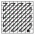The zigzag principle

If s is the side length of the square, then the zigzag value m (= 1, 2, ..., s²) corresponding to the point (i, j) (i, j = 0, 1, ..., s-1) can be calculated with this program:

k = i + j
if k < s then
	begin
		l = (k * (k + 1)) div 2
		if k mod 2 = 0 then
			m = l + i + 1
		else
			m = l + j + 1
	end
if k = s then
	m = (s - 2) * (s - 2) + i
if k > s then
	begin
		k = 2 * s - 1 - k
		l = s * s - (k * (k + 1)) div 2
		if k mod 2 = 0 then
			m = l + (s - i)
		else
			m = l + (s - j)
	end

The compression and encoding

The compression of the file

For each sxs-square and for each of the three YCbCr coordinates (or components) we have, after the cosine transform and the quantization, a sequence of s² integers ordered after the zigzag principle. In each of these sequences we have replaced the first number - the DC term - by its derivation from the preceding DC term (that of the preceding sxs-square and the same component). However, because most of these integers (when the square runs through the picture) are usually zero, it is expedient to introduce them into the file in a certain way, namely by letting every second integer be a true number and every other integer be a number of zeros (in an unbroken chain). The integers (in the new sequence) can be negative and of any size, and it is now our task to convert the integers to sequences of bits that are as short as possible. As a file consists of bytes, we must hereafter divide the resulting stream of bits into 8-blocks and convert these to bytes.

Since the integers are allowed to be of any size, we must express each integer as a pair of two sequences of bits, the first being a sequence which in some way (possibly in a coded form) corresponds to a natural number stating the length of the second sequence, which is the binary digit expression of the number in question. The first sequence of bits could simply be the binary expression of the natural number, but then these sequences would have to have the same length, for instance 4. As 4 bits can express natural numbers from 1 to 16, and since by using no more than 16 bits we can express integers up to 2¹⁶-1 = 65535, this method can be used for a picture which is fairly varied in colours or which is not too large. If you write a JPEG program, you should begin with this method, and first introduce one of those described below when the program works, because it is a simple method which can compress an appropriate photo to 15 percent of its size in BMP. But the 4 bits must be extended to 5, if the program is to be able to handle all sorts of pictures, and even 4 bits are too many bits to spend on stating these lengths, since most of the lengths are rather short. It would be preferable if we had a method that allowed the length of the first sequences (of the pairs) to vary.

Our numbers (stating numbers of bits) are natural numbers, and we want to represent them by sequences of bits in such a way that the most frequently used numbers correspond to the shortest sequences, and we must have a method that makes us able to determine when a sequence terminates. The first description of a principle that can put the elements of a given set (in our case the set of the natural numbers) into a one-to-one correspondence with sequences of bits, so that the length of a sequence is inverse proportional to the frequency of use of the element, is Shannon and Fano's method of coding from 1949.

The coding of Shannon and Fano

Assume that we have a procedure the result of which is a long reeling-off of information, which is expressed by using the elements of a given set. We want this set replaced by a set consisting of sequences of bits, in such a way that the most used sequences are the shortest. To this end, you can do the following: divide the set up in two parts so that the elements in each part are used with approximately the same frequency. For the elements in the first part, let the sequences begin with 0, and for the elements in the second part, let the sequences begin with 1. Divide each of these two sets up in two parts, so that the elements in each part are used with approximately the same frequency, and let the next bit be 0 for the elements in the first parts, and 1 for the elements in the second parts, and so on.

In our case the set in question is the set of natural numbers, and the meaning of such a number is that it states the length of the binary digit expression of an integer. The frequencies of use of the natural numbers are in some way inverse proportional to their size, and we ought to theorize about the frequencies, or test a number of random pictures and take average values. However, in this case we will only make a guess determined by our desire to get a simple formula: we assume that (the elements of) {1, 2, 3} come with the same frequency as the rest, that {1} comes with the same frequency as {2, 3}, that {4, 5} come with the same frequency as {6, 7, ...}, that {6, 7} come with the same frequency as {8, 9, ...}, and so on. With these assumptions, coding of the natural numbers will look like this:

1 00

2 010

3 011

4 100

5 101

6 1100

7 1101

8 11100

9 11101

10 111100

11 111101

12 1111100

13 1111101

etc.

Note that for n larger than 3, the number of 1's before the first 0 is the whole part of n/2 minus 1, and after this 0, there is only one bit more: 0 for n even and 1 for n odd. When (in the stream of bits) we know that some of the following bits form such a block of bits, we can easily determine when it terminates, as well as determine the corresponding natural number: if the first bit is 0, a bit more will follow; if this is 0, the number is 1, if it is 1, a bit more will follow; if this is 0, the number is 2, if it is 1, the number is 3. If the first bit is 1, we count the number of 1's before the first 0, and we know that the sequence terminates just after this 0. We add 1 to the number of the 1's and multiply this number by 2. The natural number, then, is this number, if the last bit is 0, and the succeeding number, if the last bit is 1.

The integers that are the result of the cosine transform and the quantization (s² integers for each sxs-square and each component), when the squares run through the picture, have been written in a certain way, namely so that every second integer is a true number and every other integer states a number (possibly zero) of zeros. Furthermore, we have written these integers as sequences of bits each having two parts: the first part is written in a coded form and corresponds to a natural number the purpose of which is to state the number of bits in the second part, being the binary digit expression of the integer in question. But since the integers (of the "true" type) can be negative, we must indicate this in some way. You probably think that we have to use an extra bit for this, however this is not necessary: the first digit of the digit expression (being the most significant digit) will always be 1, and we can indicate that the number is negative by replacing this 1 by a 0. The resulting stream of bits is ultimately divided up in 8-blocks, which are written into the file as bytes - possibly extending the very last block (by 0's or by 1's) so that it becomes an 8-block.

We have used this simple method of coding in our demonstration program, and as it can compress a well suited photo to 6-12 per cent of its original size, we cannot here see any reason for choosing a method involving more machinery. Nonetheless, we will now say a little about the method of coding used by JPEG (and explained in details in part two).

The coding of Huffman

If we had spent more time studying frequencies, we could have got a more efficient program. However, the method of Shannon and Fano is not the best method. The most efficient method of coding is that of Huffman, invented in 1951. This method has been almost universal in the JPEG procedure. We will describe it in part two, and the reader will understand why we have avoided it here: it is not easy to describe and illustrate, and the encoding and the decoding demand more operations. Besides, in the JPEG procedure the DC numbers and the AC numbers are Huffman-coded in a different way, and the Y component and the colour components use different Huffman tables.

The coding method of Huffman can be proved to be the most efficient one, but this superiority presupposes that all the data are encoded in the same way, and this is not the case in the JPEG compression. Therefore, the JPEG committee prescribed, besides the Huffman coding, the so-called arithmetic coding, which can compress pictures a little bit more. However, the arithmetic coding is slower and it has not been used much - partly because it has been patented.

The decoding and drawing

The program that draws the picture from the file must do all the things that we have done in the opposite order. The width and the height of the picture and the quality factor(s) must be read from a header.

Let us sum up what must be done in the construction of the data part of the file:

Divide up the picture in sxs-squares

For each square:

For each point, convert the RGB values to YCbCr values

For the Y, Cb and Cr component, cosine transform the s² numbers

Order these 3 x s² numbers after the zigzag principle

Replace the first number of an s²-sequence (the DC term) by its derivation from the analogues number for the preceding square

Quantize the 3 x s² numbers

In the resulting sequence of integers, replace each unbroken sequence of zeros by its length (possibly 0)

Write each integer as a sequence of bits (having two parts: a code and a digit expression), so that the sequences can be joined together into a continuous stream of bits.

After the header (stating the width and the height and the quality factor) has been read, we must convert each read byte of the file to an 8-block of bits, and then decode the resulting stream of bits. Each sequence of bits determining an integer consists of two parts. The first part forms a code, which is designed so that we can see where it ends. We decode it, and in this way get a natural number m. The second part of the sequence is the next m bits in the stream, and these m bits are the binary digit expression of an integer. However, if this sequence begins with 0, this indicates that the integer is negative, and the 0 must be replaced by 1. Every second integer (being non-negative) states a number of zeros, and we (imagine that we) write down these zeros. We do this until we have numbers enough to draw an sxs-square of the picture, namely 3 x s² numbers. These 3 x s² numbers are obtained by cosine transform and by quantization of the s² colour values for the three components. They must first be de-quantized by multiplying by the numbers we have divided by. After this the very first number of each s²-sequence (the DC term) must be added to the corresponding number for the preceding sxs-square, as these numbers represent differences. By the inverse zigzag procedure, each of the three s²-sequences is converted to a sxs-matrix of numbers g(u, v), u, v = 0, 1, ..., s-1, and to this matrix the inverse cosine transform is applied, giving a matrix f(i, j), i, j = 0, 1, ...,s-1, of colour values for the Y, Cb and Cr component. For each point (i, j) in the sxs-square, the three colour values f(i, j) make up an YCbCr triple, which is converted to a RGB triple, and the point in the picture corresponding to the point (i, j) in the square is coloured with these RGB values.

Miscellaneous

Leave out the last terms?

After quantization, the last of the s² numbers of the sxs-matrices g(u, v) are usually very small, and we could choose one of the numbers r = 3, 4, ..., s-1 and omit those pairs (u, v) for which u or v >= r, so that we only had to deal with r² numbers (u, v = 0, 1, ..., r-1). However, we do not win much by doing this, since r must be rather near s-1 and since the actual size of the number of zeros is not essential (30 zeros engage 8 bits and 12 zeros engage 7 bits). In the drawing procedure we could save time by restricting the inverse cosine transform to r² numbers. We have done this in our (two) drawing programs of part two (we have set r = 6). But as such a program (for practical use) has to be written in assembly language, we do not win much by doing this either, since nowadays the picture is drawn pretty fast. But it is illustrative to see how many, or rather, how few of the cosine transformed numbers (the terms in the expansion of the colour value function) we actually need. We have therefore designed our drawing program so that we can enter a "number of terms" (the number r). In this picture (using 8x8-squares) the number of terms is 8 and 4, respectively:

8 terms
4 terms

Note that the size of the file depends strongly on the fact that most of the numbers before the compression are zeros, because every second number states a number of zeros. Therefore, if there were only few zeros, the most (every second) of these numbers (being zero in coded form = 000), would unnecessarily occupy considerable space. Thus, if instead of dividing by a large number in the quantization, we divide by a small number (e.g. 0.1), we get the result that the file takes up twice as much space as in BMP format!

Why only 8x8-squares?

The choice (in the true JPEG procedure) of 8 as side length of the small squares, has nothing to do with the role of 8 in the computer, since the numbers are converted to sequences of bits of all sorts of lengths. The side length must not be too small, because then the effect of the cosine transform is lessened, and not too large either, because then the number of calculations may be too large: for an sxs-square, the total number of terms is s⁴, because there are s² points and for each point the formula has s² terms. Therefore, if the side length is doubled, the number of calculations quadruples. The choice of 8 as side length was surely the most optimal when the JPEG procedure was introduced. However, nowadays, as the speed has multiplied, we could make better compression by choosing a larger side length (12, for instance), but it is too late to alter this and the benefit is not significant.

As regards the earlier mentioned quadratic picture of 280 pixels (to demonstrate the cosine transform), the number of calculations is 1225 times larger than if the picture were divided up in 8x8-squares.

In the two pictures below we have used divisions up in 20x20- and 10x10-squares, respectively. The procedure is not as efficient for small divisions as for large ones. Both of the pictures are quantized by approximately the same numbers, the first takes up 13 Kb, the second takes up 22 Kb:

20x20-squares

10x10-squares

The luminant contra the chromatic part

Let us see how it goes if we make large differences in the quantization of the luminant and the chromatic part of the top-most picture below. In the left-most picture the quality is low for the luminant part and high for the chromatic part. Therefore the pattern is disturbed but the colours seem correct. In the right-most picture it is the opposite: the pattern is correct but the colours are unfamiliar:

Original

Bad luminant part
Bad chromatic part

Difficult pictures

The JPEG procedure always introduces changes into the picture, but by choosing a high quality, these changes can be made microscopic. But they are there, and if you want to someday be able to work up a picture, you should not save it in JPEG format. Some pictures are less suited for JPEG compression than others, in the sense that the quality must be set high, if you want the changes to be completely invisible. But it is always possible to save in JPEG without visible changes, people will say. However, this is not necessarily true: it depends on the JPEG implementation. Our demonstration program can always make a file resulting in a (nearly) faultless picture, but this is because we handle the colour components in the same way as the Y component - we only quantize by different numbers, but we could refrain from quantization (setting the quality to 100). In the true JPEG procedure it is possible to reduce the size of the two colour "pictures" (the colour components) compared to the grey scale picture (the Y component). This can be done (for instance) by a previous dividing up of the two colour "pictures" in 2x2-squares and by regarding such a square as one pixel by taking the average value of the four colour values, so that the colour pictures become four times as small. This is done before the dividing up in 8x8-squares, so that four 8x8-squares of the Y component are combined with one 8x8-square of the colour components. The reason is that the colours usually do not vary rapidly across the picture, and we can compress about 25 per cent more in this way. The procedure is called subsampling (of the colour components).

The next two pictures are made with our (home-made but) true JPEG program in part two, but with different settings. The picture is made by laying a picture for which every second pixel is green and every other pixel is transparent over another picture. Both pictures take up rather much space because of the strong changes from pixel to pixel. In the first picture the colour components are handed in the same way as the Y component, therefore the picture is correct. In the second picture subsampling of the colour components has been used, so that the colour values become average values, therefore the picture is more green:

Without subsampling

Subsampling

Note that not all JPEG compressing programs allow for the option between subsampling and non-subsampling the colour components.

For a picture in grey scale we have only the Y component, but as the contribution of the Cb and Cr components (after quantization) are small compared to the Y component, the grey scale version of a picture takes up almost as much space as the colour version - usually more than 90 per cent.

The compression should reach its extremum when the picture is of only one colour. This is the case for our demonstration program: the data part of such a 1000x1000-pixel picture take up only 14 bytes. But when we use the true JPEG procedure, the data part will take up 15.000 bytes - we will see why in part two.

Transparency

Some image formats can contain transparency, GIF and PNG, for instance, but not BMP and JPEG. GIF is especially suited for graphic representations and PNG is suited for pictures with objects laid over a simple background. They are both lossless, but a GIF picture can only contain 256 different colours (specified in the header), and, in spite of an effective compression, a photo converted to a PNG file often takes up 75 per cent of the BMP file. As regards JPEG, in a FAQ-article you can read the following answer to the question "Can I make a transparent JPEG?": "No. JPEG does not support transparency and is not likely to do so any time soon. It turns out that adding transparency to JPEG would not be a simple task; read on if you want the gory details". And then we are told that in a GIF picture the transparency is introduced by letting an unused colour value mark out the transparent domain, but this method cannot be used in JPEG. It could be used in BMP, where one of the 16777216 possible colours could easily be missed for marking out a transparent domain; however not in JPEG, where the colour values are imprecise. Transparency will engage one bit for each point, and this new component could be subjected to the same procedure as the three YCbCr components. However, this method is rejected on the grounds that the JPEG procedure is not suited for sharp passages: if the boundary around a hole, through which strongly deviating colours appear, is to be reproduced satisfactorily, the cosine transformed numbers (of the transparency component) could only be quantized by small numbers, and then the file would take up quite some space. This is true, but the picture would still take up much lesser space than in PNG format, and besides, transparency is usually only for temporary use. It is easy to arrange the JPEG file such that it can support transparency.

However, as not much is won by cosine transform and quantization of the transparency component, these operations should be left out, and the bits for the transparency should be entered in the file in this way: we go along the horizontal lines by turns from left to right and from right to left, so that the pixels are adjacent, and in this sequence of bits we replace each unbroken interval of 0's or 1's by the number of the 0's or 1's (the sum of these numbers is just the width times the height). The resulting sequence of natural numbers is then coded, and can be written in the file before the colour data. By this method, the transparent domain becomes exactly as in the original picture. In the picture to the left the black is made transparent and the picture is laid over a blue background resulting in the picture to the right, and in spite of the very low quality of this picture, the transparent domain is the same:

Original
Transparency

The procedure of introducing transparency in a picture can take place via a picture in BMP format, for instance. The BMP format does not (at present) support transparency, but we can accompany the picture by a monochrome picture also in BMP format determining the transparent domain. A monochrome picture is a picture containing only two different colours, usually black and white. The RGB values of the two colours are stated in the header (or rather the header is prolonged with the bytes necessary for this information), and the data - one bit for each point - are written in the same way as the RGB values in an usual BMP file: row for row, but such that each 8-block of bits is converted to a byte (and such that the length of the rows of bytes is divisible by 4). This method is supported by the Windows bitmap drawing procedure: if we let the transparent domain in the picture with the colours be black, and let it be the white domain in the monochrome black-and-white picture, then Windows has procedures that can transfer the data of the two files directly to the screen, making a picture where the transparent domain is empty, so that we through this see the underlying - the desktop, for instance.

Introduction

The four distinct modes of operation

The JPEG committee intended that the method should be available in a number of variants and with a number of extensions:

The sequential DCT mode of operation, where the picture is scanned in the same way as in part one (but not in our zigzag way, column-wise from left to right, but line-wise from top to bottom, just as in reading ).
The progressive DCT mode of operation, where the picture is displayed in its entirety concurrently with the transmission of the bitstream, at first imperfect and then gradually improving.
The lossless mode of operation, where the file is only compressed, with no data lost by cosine transforms or quantization.
The hierarchical (DCT or lossless) mode of operation, where the picture is stored at multiple resolutions for different uses (low-resolution screen, high-resolution printer, etc.), in such a way that the lower-resolution images are stored with supplementary data which can be added on to produce higher-resolution images as required.

The colour values are usually measured in bytes (8-bit numbers), and in this case the precision of the (real) numbers in the calculations is set to 11 bit.

JPEG also offers extended precision, primarily intended for grey scale pictures, where the colour values instead of utilizing 8 bits use 12 bits (a range from 0 to 4095), and where the precision in the calculations is increased to 15 bit. Extended precision implies that the Huffman tables must go to size 15 (instead of 11) for the DC numbers and size to 14 (instead of 10) for the AC numbers. Furthermore, the numbers in the quantization tables can be words (from 0 to 65535) instead of bytes. As this possibility is rarely used, we will ignore it here.

For the baseline sequential DCT mode, that is, the non-extended sequential DCT mode, the method of coding is the Huffman coding with two tables for each component. For the extended modes you can choose between the Huffman coding with two or four tables for each component and the arithmetic coding.

One Mode Survives

Although four modes were intended, only the baseline sequential DCT mode has survived in widespread use.

There is not much point in the progressive and the hierarchical mode nowadays, where a JPEG picture is transmitted and displayed fast.
The benefits of the lossless mode seem too minor. Arithmetic coding can compress a little better than the Huffman coding, but it is slower and there have been patent-related problems.

Software Used in Researching this Book

Our account here, like our earlier account in part one, was accompanied by the writing of some programs. This time this was done only to ensure that we had properly understood the procedure. We will show pieces of these programs written in a Pascal-like language which should be easy for everybody to understand.

We first made a program that can convert a picture in BMP format to a grey scale picture in JPEG format. When this worked correctly, we extended it to colour pictures. Such a program, to be of use in production systems for JPEG files, must of course be written in assembly language and without making use of the co-processor (80-bit numbers) in the transforms. However, if the program is only for demonstration or if it is a part of a program producing computer graphic, it may be written in a high-level language and may use floating point operations. Our program which can read a JPEG file and draw the picture, for the baseline sequential DCT mode, was made in the same way. Since there are already many such programs, it does not need to be efficient. On the contrary, we have made it extra slow by using a "setpixel" procedure, because it is simpler - and because it gives the drawing a funny look.

The picture to the left below is made with our program in part one and the right with our program in this part. The quality is approximately the same. The first takes up 16.3 Kb and the second takes up 15.1 Kb (uncompressed they take up 228 Kb):

The demo program: 16.3 Kb
The true program: 15.1 Kb

Requirements Documents

"Digital Compression and Coding of Continuous-Tone Still Images - Requirements and Guidelines/Recommendation T.81" (1992), also called just T.81, is 180 pages long. If you are only interested in the baseline sequential DCT mode with Huffman coding, you do not have to read all 180 pages. The knowledge required of mathematics and programming is limited. You must already know the meaning of the mathematical terms, since these are not explained.

The purpose of T.81 was to set a common standard for the core of the procedure. The specifics are described separately in standards for the implementation. These are in additional documents with titles like "JPEG File Interchange Format, Version ...". The only thing in our account that is in these implementation documents is the colour space designation: the RGB → YCbCr transform.

The formulas for this colour transform shown in part one can be found in version 1.02 from 1992 (7 pages). T.81 only speaks of four components. It is implicit that only one component means that the picture is in grey scale, that three components can be the RGB components or most commonly the YCbCr components, and that the fourth component is for the possibility of transparency.

The Huffman coding

The main difference between our procedure in part one and the real JPEG procedure is that in part one we used a method of coding which is easy to understand and use, but which was not very efficient, partly because it was based on frequencies that were more determined by our desire for a simple coding procedure than by reality. JPEG uses the more efficient Huffman coding and frequencies that either are determined by the actual picture or by the average values for a number of typical pictures. Furthermore, we used the same coding procedure for all the numbers, whereas JPEG uses different coding for the DC and the AC numbers and also different coding for the Y component and for the two colour components - this implying that the coding can demand tables of more than 450 numbers.

We will here choose Huffman tables based on typical frequencies, rather than on the frequencies measured by a pre-scanning of the actual picture. Therefore we only need to know how the Huffman encoding and decoding is to be performed once we have the necessary tables: we do not need to know how these tables are constructed on the basis of frequency. We will, however, show the procedure for the construction of the Huffman tables. It is a rather simple procedure, and the reader might want to make a program that measures frequencies and constructs the Huffman tables from the actual picture (we will show the programs in Appendix 2).

Assume that we have some values a1, a2, ..., an, which are attached to frequencies and which are to be equipped with code words so that the most frequently used values get the shortest codes. This can be done by constructing a so-called Huffman tree with the values as leaves with attached frequencies. Usually a Huffman tree can be constructed in several ways giving different code lengths. JPEG chooses the following:

We order the values according to decreasing frequency. For the two last values we add their frequencies, remove the two values and insert a node at the place among the remaining values where this frequency belongs (so that the frequencies are still decreasing - note that if the new frequency occurs among the others, the insertion can be made in more than one way). This is repeated until there is only one node left, and this will have frequency 1. We have for each operation removed two things: either two values, or two nodes, or a value and a node. We construct the Huffman tree by placing the values (leaves) at the bottom and successively connecting with lines the pairs of removed things with the node that has replaced them.

If, for example, the values are the numbers 0, 1, 2, 3 and 4, and their frequencies are 0.3, 0.25, 0.2, 0.15 and 0.1 (having sum 1), respectively, the removal procedure could look like this:

a1 0 0.3 0.3 0.45 0.55 1

a2 1 0.25 0.25 0.3 0.45

a3 2 0.2 0.25 0.25

a4 3 0.15 0.2

a5 4 0.1

And the Huffman tree could look like this:

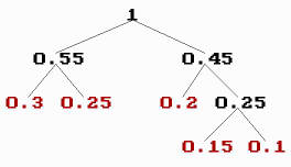Huffman tree

The length of the Huffman code assigned to a value is the number of lines from the value to the last node (the top node with frequency 1). Once we know the lengths (of the codes) assigned to the values, we can form the code words, and this can be done in different ways:

By using the Huffman tree, we can code for instance by writing 1 when we go to the right and 0 when we go to the left when we progress from the value towards the top node:

0 00

1 10

2 01

3 011

4 111

But we can also code without the Huffman tree, what is essential is the code lengths for the values. For instance, we can code so that the sequence of code words (identified by numbers via their binary digit expressions) is increasing: forming consecutive numbers when the code length is unaltered and adjoining zeros when the code length increases:

0 00

1 01

2 10

3 110

4 111

It is this last way of forming codes that is used by JPEG, because it is fast to decode.

In JPEG a code word must not consist of only 1's. We can avoid this by adding provisionally an extra value whose frequency is half (for instance) of the frequency of the last and least value (and finally remove a code from the codes of the largest length).

Furthermore, the length of a code word must not exceed 16. Therefore, if the Huffman tree leads to code lengths of more than 16 bits, the longest codes must successively be shortened. In our case, where we have imported the coding, we do not need to care about this problem, but we will briefly describe it: the longest code length is assigned to an even numbers of values. Therefore we can shorten the longest length by one bit (the last) and assign this code to one of the values, if we can find another (shorter) code to the other value. Assuming that the last (longest) codes with fewer bits have j bits, we can remove the last of these codes (of length j) and extend it by a 0 and a 1, respectively, so that we get two new codes of length j+1 which can replace the two removed codes.

The Huffman coding is performed from the (Huffman) values (occurring in the picture) and the code length assigned to each value (determined by its frequency). Therefore our point of departure is two lists of bytes: the first, called BITS, goes from 1 to 16, and tells us, for each of these numbers, the number of codes of this code length. The second, called HUFFVAL, reels off, for each code length having a non-zero number of codes, the values to be coded with codes of this length (and as many values as there are codes of this length). The values in HUFFVAL are called the Huffman values, and they are ordered according to increasing code length (within a given code length the ordering is arbitrary).

In our program we use these lists for the DC numbers of the Y component:

BITS

0 1 5 1 1 1 1 1 1 0 0 0 0 0 0 0

HUFFVAL

0

1 2 3 4 5

6

7

8

9

10

11

and these lists for the DC numbers of the two colour components:

BITS

0 3 1 1 1 1 1 1 1 1 1 0 0 0 0 0

HUFFVAL

0 1 2

3

4

5

6

7

8

9

10

11

The last lists tell that there are: 0 codes of length 1, 3 codes of length 2 (coding the Huffman values 0, 1 and 2), 1 code of length 3 (coding the Huffman value 3), etc.

Most of the numbers to be coded are AC numbers, and they are coded in another way than the DC numbers. Moreover, the values range a larger interval. As we import the Huffman coding, we must use lists containing all the possible values.

In our program we use these lists for the AC numbers of the Y component:

BITS

0 2 1 3 3 2 4 3 5 5 4 4 0 0 1 125

HUFFVAL

1 2

3

0 4 17

5 18 33

49 65

6 19 81 97

7 34 113

20 50 129 145 161

8 35 66 177 193

21 82 209 240

36 51 98 114

130

9 10 22 23 24 25 26 37 38 39 40 41 42 52 53 54 55 56 57 58 67 68 69 70 71 72 73 74 83 84 85 86 87 88 89 90 99 100 101 102 103 104 105 106 115 116 117 118 119 120 121 122 131 132 133 134 135 136 137 138 146 147 148 149 150 151 152 153 154 162 163 164 165 166 167 168 169 170 178 179 180 181 182 183 184 185 186 194 195 196 197 198 199 200 201 202 210 211 212 213 214 215 216 217 218 225 226 227 228 229 230 231 232 233 234 241 242 243 244 245 246 247 248 249 250

and these lists for the AC numbers of the two colour components:

BITS

0 2 1 2 4 4 3 4 7 5 4 4 0 1 2 119

HUFFVAL

0 1

2

3 17

4 5 33 49

6 18 65 81

7 97 113

19 34 50 129

8 20 66 145 161 177 193

9 35 51 82 240

21 98 114 209

10 22 36 52

225

37 241

23 24 25 26 38 39 40 41 42 53 54 55 56 57 58 67 68 69 70 71 72 73 74 83 84 85 86 87 88 89 90 99 100 101 102 103 104 105 106 115 116 117 118 119 120 121 122 130 131 132 133 134 135 136 137 138 146 147 148 149 150 151 152 153 154 162 163 164 165 166 167 168 169 170 178 179 180 181 182 183 184 185 186 194 195 196 197 198 199 200 201 202 210 211 212 213 214 215 216 217 218 226 227 228 229 230 231 232 233 234 242 243 244 245 246 247 248 249 250

If we call the number of Huffman values nhv, we have an array HUFFVAL[k] from k = 1 to nhv arranging the Huffman values in their enumerated order. From the list BITS[i] we form an array HUFFSIZE[k] from k = 1 to nhv of the code lengths i for which the number BITS[i] is non-zero, each i repeated BITS[i] times, so that the array HUFFSIZE[k] is parallel to HUFFVAL[k]. And we now construct an array HUFFCODE[k] from k = 1 to nhv stating the Huffman code assigned to HUFFVAL[k]. We identify a code with the integer having the bits of the code as binary digit expression (e.g. 110 = 6), being aware that as the code can start with one or more zeros, the digit expression must start with zeros in order to get the right length (e.g. 011 = 3).

The code words are generated in this way: assume that we have formed all the codes of length <= n, and that the last formed code is the number c. Now assume that the next code length is n+i, then the next code is c = 2ⁱ∙(c + 1) (the code got by joining i zeros to c + 1), and the following codes are the consecutive numbers (c+1, c+2, ...), so many as there are codes of (the new) length n = n+i. At the start c is set to 0. Code number k, HUFFCODE[k], is the code assigned to the Huffman value HUFFVAL[k].

The encoding

For the encoding we reorder the lists (arrays) HUFFSIZE and HUFFCODE so that they become functions of the Huffman values (instead of functions of the order number), forming arrays EHUFSI[val] and EHUFCO[val]:

if val = HUFFVAL[k] then

EHUFSI[val] = HUFFSIZE[k] and

EHUFCO[val] = HUFFCODE[k]

Note that EHUFCO[val] is an array: EHUFCO[val][j] is the j-th bit of the code.

If we let the function size(n) (n integer) state the number of digits in the binary digit expression of n, and let digit(n) be the digit expression itself (so that digit(n) is an array of bits from 1 to size(n)), the procedures for the construction of HUFFSIZE[k], HUFFCODE[k], EHUFSI[val] and EHUFCO[val] (and which are to be applied for each Huffman table) could look like the following:

k = 1

i = 1

j = 1

1

if j <= bits[i] then

begin

huffsize[k] = i

k = k + 1

j = j + 1

goto 1

end

i = i + 1

j = 1

if i <= 16 then

goto 1

nhv = k - 1

k = 1

c = 0

i = huffsize[k]

2

huffcode[k] = c

c = c + 1

if k = nhv then

goto 4

k = k + 1

if huffsize[k] = i then

goto 2

3

c = 2 * c

i = i + 1

if huffsize[k] = i then

goto 2

else

goto 3

4

k = 1

5

val = huffval[k]

e = huffsize[k]

ehufsi[val] = e

l = size(huffcode[k])

dig = digit(huffcode[k])

if l < e then

for j = 1 to e - l do

ehufco[val, j] = 0

for j = 1 to l do

ehufco[val, e - l + j] = dig[j]

k = k + 1

if k <= nhv then

goto 5

For the lists above for the DC numbers for the Y component, nhv = 12, HUFFSIZE[k] is the sequence 2 3 3 3 3 3 4 5 6 7 8 9, and HUFFCODE[k] is the sequence 00, 010, 011, 100, 101, 110, 1110, 11100, 111000, 1110000, 11100000, 111000000. And for the functions EHUFSI[val] and EHUFCO[val], we have: EHUFSI[0] = 2, EHUFSI[1] = 3, EHUFSI[2] = 3, etc., and EHUFCO[0] = 00, EHUFCO[1] = 010, EHUFCO[2] = 011, etc.

In the encoding we must for non-negative integer n know how many digits are in the binary expression of n. The function size(n) states this number, and it is extended to negative n by letting -n have the same size as n. It is given by size(0) = 0 and size(n) = trunc(ln(abs(n)) / ln(2)+0.000001) + 1 for n <> 0:

n size

0 0

1 1

2, 3 2

4 ... 7 3

8 ... 15 4

16 ... 31 5

32 ... 63 6

64 .. 127 7

128 .. 255 8

256 .. 511 9

512 .. 1023 10

1024 .. 2047 11

etc.

The integer the binary digit expression of which follows a Huffman code, can be negative, and (as explained in part one) we do not need an extra bit to indicate this: the digit expression will always begins with 1 and we can write 0 instead of the 1. At the decoding of the sequence, the start with 0 will then show that the number is negative, and 1 followed by the rest of the digits will be the binary expression of the numerical value. However, in order to indicate that the number is negative, JPEG has chosen to replace all the digits by their opposite bit (forming the complement of the number). Therefore, if the digit expression begins with 0, has val digits and corresponds to the (non-negative) integer n, then the negative integer is -(2^val - 1 - n) (in T.81 it is said that if the sequence of digits begins with 0 and if the number of digits is T, then we get the numerical value by adding 2^T + 1 to the number, but this is not correct, the number of course is obtained by subtracting it from 2^T - 1 = 11...1 (T figures 1)).

The program for the function, digit(n) (n <> 0), giving the binary digit expression for the integer n, when n is positive, and the complement to the digit expression, when n is negative, could look like this:

j = size(n)

if n < 0 then

n = round(exp(j * ln(2))) - 1 - abs(n)

if j = 1 then

digit[1] = n

else

begin

j = j - 1

q = round(exp(j * ln(2)))

i = 0

while i <= j do

begin

i = i + 1

l = n div q

n = n - l * q

q = q div 2

digit[i] = l

end

The DC numbers: For a DC number (the first number of the 64-array) it is not the number itself, but the difference DIFF between the number and the preceding DC number which is to be coded, and it is not DIFF itself, but the number val of bits needed to express it: val = size(DIFF). The code is then EHUFCO[val] and after this comes the val binary digits of DIFF: digit(DIFF)[j], j = 1, ..., val.

The AC numbers: The 63 AC numbers (of the 64-array) are encoded in another way than the DC number. Here the size of the actual number (not a difference) is coded, and since there are usually many zeros in an AC array, the number of these in an uninterrupted row is combined with the size of the following non-zero AC number. If there are m zeros before the non-zero AC number n and if the size of n is k, we combine these two numbers (being half bytes) to the byte val = m*16 + k, and it is this byte that is Huffman coded. This presupposes, however, that m and k really are half bytes (that is, <= 15). k is always <= 11, but there can be more than 15 zeros in a row, therefore, when a row of zeros has reached 15 and is followed by another zero, we must code these 16 zeros separately: the byte to be coded is val = 15*16 + 0 = 240 (called ZRL). If the last of the 63 AC numbers is zeros, this is indicated by writing the Huffman code assigned to val = 0*16 + 0 = 0 (called EOB, End-Of-Block). After the Huffman code has been written, the k binary digits of the non-zero AC number are written in the same way as for the DC (or rather the DIFF) numbers. Frequencies and code lengths are assigned to all the (Huffman) values val = m*16 + k that are constructed in this way (or at least those values occurring in the picture). The number of Huffman values (to be coded) can at most be the number of possible zeros (0, 1, ..., 15, that is, 16) times the number of possible sizes of the non-zero AC numbers (namely 10), and in addition to this product (160), the two extra values 240 and 0. In total 162 Huffman values. As we here have chosen to import Huffman tables based on tests of a number of casual pictures, our AC Huffman tables most contain 162 values.

The decoding

For the decoding (when the file is read)(instead of the arrays EHUFSI[val] and EHUFCO[val]) we must have constructed beforehand three arrays from k = 1 to 16: the minimum (first) code of length number k, MINCODE[k], the maximum (last) code of length number k, MAXCODE[k], and the number of MINCODE[k] in the sequence of the codes (and Huffman values), VALPTR[k] (value pointer):

j = 0

k = 0

0

k = k + 1

if k > 16 then

goto fin

if bits[k] = 0 then

begin

maxcode[k] = -1

goto 0

end

j = j + 1

valptr[k] = j

mincode[k] = huffcode[j]

j = j + bits[k] - 1

maxcode[k] = huffcode[j]

goto 0

fin

Note that when there are no codes of code length k, MAXCODE[k] = -1, and MINCODE[k] and VALPTR[k] are not defined.

Decoding then goes on as following: In the stream of bits, the first thing to do is to collect as many together that they form a code: we must determine where to stop. We start with k = 0, c = 0 and MAXCODE[0] = -1 (so that c > MAXCODE[0]), and for each read bit we join this to c and increase k by 1, until c <= MAXCODE[k]. Since we identify codes with numbers, the joining means that we set c = 2*c + bit for each new bit (called bit). The code then is c, and we shall find the Huffman value val assigned to c, and this is the Huffman value having the number k = VALPTR[k] + c - MINCODE[k], so that val = HUFFVAL[k]:

k = 0

c = 0

while c > maxcode[k] do

begin

nbit

c = 2 * c + bit

k = k + 1

end

val = huffval[valptr[k] + c - mincode[k]]

Here nbit is the procedure described later, which reads the next bit.

The header part

The markers

The header part of a JPEG file is divided into segments, and each segment starts with a marker, identifying the segment. Usually a JPEG file contains 7 different markers. A marker is a pair of bytes, the first is 255 and the second is different from 0 and 255. We identify a marker by its second byte. Two markers stand alone (and thus do not open a segment): the marker which opens the file SOI (Start Of Image) = 216 and the marker which closes the file EOI (End Of Image) = 217. (There is one more type of marker which stands alone, but this is not used in the sequential DCT mode which we restrict ourselves to here: it marks a restart of a scanning and it is indexed by one of the numbers 0, 1, ..., 7: RST0, ..., RST7 (ReSTart) = 208, ..., 215). The other markers open a segment, and in this case the following pair of bytes (b1, b2) states the length l of the segment (including these two bytes): l = b1 * 256 + b2. The following sequence of l - 2 bytes is the content of the segment. There are the following types of segments (identified with their markers):

APP0, APP1, ..., APP15 (APPlication) 224-239

COM (COMment) 254

SOF (Start Of Frame) 192-207, except 196, 200 and 204

DHT (Define Huffman Table) 196

DQT (Define Quantization Table) 219

SOS (Start Of Scan) 218

(and a few more, which are not used here: DNL (Define Number of Lines = 220), DRI (Define Restart Interval = 221), DHP (Define Hierarchical Progression = 222), EXP (EXPand reference component(s) = 223), DAC (Define Arithmetic Coding conditioning(s) = 204), TEM (for TEMporary use in arithmetic coding = 1) and besides some reserved markers: JPG (reserved for JPeG extensions = 200, 240, 241, ..., 253) and RES (REServed = 2, ..., 191))

The first two - APP and COM - specify things that lie outside the proper JPEG procedure. Usually only a single APP segment is present (namely APP0), specifying the implementation. An APP segment can also contain information on camera type and on when the picture was taken. COM can state the program used to make the file, the chosen quality per cent, etc.

The frame segment SOF

The point of departure of the JPEG procedure is a "picture", and a picture can be defined as a (rectangular) matrix of either numbers, pairs of numbers, triples of numbers or quadruples of numbers. That is, a picture is a matrix of arrays having one of the numbers 1-4 as length. A grey scale picture is a matrix of bytes. A colour picture is a matrix of RGB triples (of bytes) or of YCbCr triples (of signed bytes). A picture can thus be regarded as consisting of one or more (at most four) matrices of integers, and such a matrix is called a component of the picture. To each component is assigned a component identifier (byte): for instance 0 for the (one) component of a grey scale picture, and 0, 1 and 2 for the three components of a colour picture.

The dimensions of the picture, the component identifiers and the order of the components are specified in the frame segment SOF, along with how the components are to be handled in relation to each other. Because the colours usually only alter slowly from place to place (and as we are not very good at distinguishing small alterations in colours), for the two colour components, we can, for instance, divide the picture up in 2x2-squares of pixels and take the average values, so that we regard such a square as one pixel and thus deal with colour pictures that are four times as small. We can also restrict ourselves to two pixels, either lying horizontally or vertically. A pair of numbers (Hi, Vi) for each component determines how the components are to be scanned in relation to each other. Hi and Vi can go from 1 to 4 (Hi and Vi must be rather small: the sum of their products must not exceed 10). Let H and V be the maximum Hi and Vi value, respectively. These maximum values are usually linked to the Y component, and this ((Hi, Vi) = (H, V)) means that the pixels are taken as they are: there are as many samples horizontally as the width of the picture, and there are as many horizontal lines as the height of the picture. If a (colour) component has the pair (Hi, Vi), the number of samples in a horizontal line is (Hi/H) times width, and the number of sampling lines is (Vi/V) times height, that is, small rectangles of (H/Hi)x(V/Vi) pixels are collected (and regarded as one pixel). Usually (Hi, Vi) = (1, 1) for the two colour components, and (Hi, Vi) = (1, 1) or (2, 1) or (1, 2) or (2, 2) for the Y component. (Hi, Vi) = (2, 2) means that four colour pixels are collected and that "this" pixel is combined with four Y pixels. As the picture is divided up in 8x8-squares, this means that four 8x8-squares for the Y component are combined with one 8x8-square for the colour components. The coded data (the coded 64-arrays) for the four Y squares are written in the file in the usual scanning order: from left to right along the lines, and from top to bottom. Next comes the coded data (the coded 64-arrays) for the two colour components. The analogue procedure when only two pixels are collected (horizontally or vertically). Such a part of the data stream arising from all the components and the collected 8x8-squares is called a minimum coded unit (MCU).

This picture shows the drawing (pixel for pixel - and on an enlarged scale) when four Y component 8x8-squares are collected - you are to image four 8x8-squares in the centre, the two (uppermost) have been drawn, the third is being drawn:

The drawing

The two pictures below the following picture (which takes up 3.2 Kb) are this picture with every second vertical line drawn black, but scanned in different ways: for the colour components, two pixels are collected in the vertical and the horizontal direction, respectively (that is, (Hi, Vi) = (1, 1) for the colour components, and (Hi, Vi) = (1, 2) and (2, 1) for the Y component). In the first picture (which takes up 5.9 Kb) the colours are correct, in the second picture (which takes up 4.7 Kb) the colours are faded, because they are mixed with the black of the lines:

Original

Vertical subsampling

Horizontal subsampling

The frame segment SOF consists of the following bytes: the marker (255, b), where the byte b specifies the scanning mode. We assume here that b = 192, meaning the baseline sequential DCT mode; then the pair of bytes stating the length of the segment (including these two bytes), this pair is (0, 8 + 3 * the number of components); then a byte stating the number of bits of the colour values, here set to 8 (meaning that the colour values are bytes), but it is 12 for the extended mode; then a pair of bytes (b1, b2) stating the height (= b1 * 256 + b2) of the picture and a pair of bytes stating the width; and finally a byte stating the number of components (1-4), and for each component these bytes: the component identifier (byte), Hi (½ byte) and Vi (½ byte)(byte = Hi * 16 + Vi) and the quantization table destination selector (byte).

The pair (Hi, Vi) is here (1, 1) for the colour components and (1, 1), (1, 2), (2, 1) or (2, 2) for the Y component. The quantization table destination selector is one of the numbers 0-3, for instance 0 for the Y component and 1 for the colour components.

The Huffman table segment DHT

Usually there are two Huffman table segments in the file for a grey scale picture and four for a colour picture: for each component the DC and the AC numbers are coded differently, and the Y component and the two colour components are coded differently. In a Huffman segment the information (after the marker and the pair of bytes stating the length) is arranged in this way: the first half byte is 0 if the Huffman tables are for DC numbers and 1 if they are for the AC numbers. The next half byte is the Huffman table destination identifier (0 or 1), for instance 0 for the Y component and 1 for the colour components (to be referred to in the scan segment SOS where the Huffman tables are specified). The following sequence of 16 bytes is the list BITS, stating for i = 1, ..., 16 the number of codes of length i. And then comes the list HUFFVAL of Huffman values: for each code length different from zero, there will be just as many values as there are codes of this length. If we call the number of Huffman values nhv, the number of bytes in the segment (including the pair stating the length) is 19 + nhv.

The Quantization table segment DQT

A quantization table is an 8x8 matrix of bytes ordered after the zigzag principle. There are usually different quantization tables for the Y component and for the colour components. In the annex "Examples and guidelines" of T.81 you can find the following for respectively the Y component and the colour components:

16 11 10 16 24 40 51 61

12 12 14 19 26 58 60 55

14 13 16 24 40 57 69 56

14 17 22 29 51 87 80 62

18 22 37 56 68 109 103 77

24 35 55 64 81 104 113 92

49 64 78 87 103 121 120 101

72 92 95 98 112 100 103 99

17 18 24 47 99 99 99 99

18 21 26 66 99 99 99 99

24 26 56 99 99 99 99 99

47 66 99 99 99 99 99 99

99 99 99 99 99 99 99 99

It is mentioned that "If these quantization values are divided by 2, the resulting reconstructed image is usually nearly indistinguishable from the source image". With our program "JPEG_File" you can see the tables for a picture (using the sequential DCT procedure and) given the name "pict". In our program to produce a (true) JPEG file we have chosen another table for the Y component than the above, namely the following used in an image editing program (IrfanView), by setting the quality to 70 per cent:

10 7 6 10 14 24 31 37

7 8 11 16 35 36 33

8 8 10 14 24 34 41 34

10 13 17 31 52 48 37

11 13 22 34 41 65 62 46

14 21 33 38 49 62 68 55

29 38 47 52 62 73 72 61

43 55 57 59 67 60 62 59

A quantization table is specified in a DQT segment. A DQT segment begins with the marker DQT = 219 and the length, which is (0, 67). Then comes a byte the first half of which here is 0, meaning that the table consists of bytes (8 bit numbers - for the extended mode it is 1, meaning that the table consists of words, 16 bit numbers), and the last half of which is the destination identifier of the table (0-3), for instance 0 for the Y component and 1 for the colour components. Next follow the 64 numbers of the table (bytes).

The scan segment SOS

Just after the scan segment SOS come the encoded data of the picture, and the scan segment specifies the Huffman tables to be used for the components. The segment begins with the marker SOS = 218 and the length, which is (0, 6 + 2 * the number of components). Then comes a byte stating the number of components (1-4), and then for each component two bytes, the first is the component identifier (defined in the frame segment) and the second is divided up in two parts, the first stating the destination selector of the DC Huffman table and the second the destination selector of the AC Huffman table (for instance 0 for the Y component and 1 for the colour components). The segment closes with three bytes which in our case (sequential DCT) are 0, 63 and 0 (the last divided in two half bytes).

The guidelines and the implementation

The guidelines

The recommendation T.81 closes with a list of patents that may be required in relation to implementation of the arithmetic coding and the hierarchical processes (and which is probably the reason why these methods are not more wide spread) as well as a bibliography. But just before these annexes is an annex called "Examples and guidelines" (which "does not form an integral part of this Recommendation/International Standard"). In this annex you can find the quantization tables shown above and the Huffman tables we have shown and used in our (true) JPEG programs. As regards the quantization tables it is said that: "These are based on psycho-visual thresholding and are derived empirically using luminance and chrominance and 2:1 horizontal subsampling. These tables are provided as examples only and are not necessarily suitable for any particular application. These quantization values have been used with good results on 8-bit per sample luminance and chrominance images". The Huffman tables "have been developed from the average statistic of a large set of images with 8-bit precision". The annex also includes procedures for generating the lists which specify a Huffman code table, namely: 1) the procedure mentioned above for the construction a Huffman tree on the basis of frequency and how to find the code lengths from the tree and count the number of codes of each length in order to get the list BITS (and possibly revise this list, so that it goes from 1 to 16); and 2) the procedure for sorting the Huffman values according to code length to get the list HUFFVAL. Because we imagine that we have imported these lists, we will not here go into details with these procedures - we will show the programs in Appendix 2.

The implementation

The colour space designation, in our case the conversion from RGB triples to YCbCr triples (by linear transform RGB → YCbCr shown in part one), is not mentioned at all in T.81. Things like this belong to the concrete implementation of the JPEG method, and the implementation used is specified in one or more APP segments. These are two sorts of implementation: the interchange format, in which all the necessary tables are included in the file, and the abbreviated format, in which some of the tables (possibly all) are missing, because the application supplies them (possibly installed via the abbreviated format for table-specification, being a JPEG file without colour data).

Here we apply the interchange format specified in an APP0 segment having these bytes after the pair (0, 16) stating the length of the segement:

the identifier (= JFIF): the five bytes 74, 70, 73, 70 and 0 forming the string of characters "jfif#"

the version (pair): in our case (1, 2)

units (byte): 0

Xdensity (pair): (0, 1)

Ydensity (pair): (0, 1)

Xthumbnail (byte): 0

Ythumbnail (byte): 0

The X- and Ydensity is respectively the horizontal and vertical pixel density measured in dots per inch (units = 1) or dots per cm (units = 2). We have chosen X = 1 and Y = 1 and no units (units = 0) meaning that such a default print information is not present. X- and Ythumbnail is the width and the height of a thumbnail picture, respectively. We have set these numbers to 0, meaning that such a picture is not stored in the header. In the opposite case the data of this (the RGB values, for instance) must be stored in the segment just after the above bytes, or in an APP segment following this APP segment.

If there are no APP segments, you get the default implementation, which is the one we use here. A description of this implementation can be found in "JPEG File Interchange Format/Version 1.02" (1992). There are no default quantization tables and Huffman tables. If some of these are missing, it must be because an abbreviated format is used, and the tables must appear in the program to open the file and referred to in an APP segment.

Program for making a grey scale file

Now for the program that can produce a grey scale JPEG file. We assume that the width and the height of the picture are divisible by 8, and set wid8 = width div 8 and hei8 = height div 8. And we assume that the colour values are given in form of a memory-block pb of a bitmap, so that the colour value (byte) of the point having screen coordinate set (i, j) (i = 0, ..., width-1, j = 0, ..., height-1), is pb[(height-1 - j) * width + i]. More precisely: we assume that the picture is given as a colour picture in BMP format, and we use only the part of it lying within the largest domain that can be regularily divided up in 8x8-squares, and we construct pb by taking the average of the RGB values.

We have written the markers (and their segments) in this order: SOI, APP, DQT, DQT, SOF, DHT, DHT, SOS (there are two of the DQT and DHT segments, because there are two quantization tables and two Huffman codings). The last segment - SOS - marks the beginning of the stream of the encoded data, and after this the file closes with the marker EOI. We have for the DC and for the AC numbers calculated the arrays EHUFSI[val] and EHUFCO[val][i] of the size of the code assigned to the Huffman value val and the code itself. In the program these arrays are called ehufsid[val] and ehufcod[val] for the DC numbers, and ehufsia[val] and ehufcoa[val] for the AC numbers.

For the 8x8-square having coordinate set (i0, j0) (i0 = 0, ..., wid8-1, j0 = 0, ..., hei8-1) and for the point in the square having coordinate set (i, j) (i, j = 0, ..., 7), the screen coordinate set is (i0 * 8 + i, j0 * 8 + j). For each 8x8-square we have an 8x8-matrix f of colour values (signed bytes - we have subtracted 128 from the original colour values (level shift) in order to get smaller numerical values), and by discrete cosine transform and quantization and round off, we get an 8x8-matrix g(u, v) of integers. This procedure (or rather, function) is called costrans(f): g = costrans(f). The inverse of the zigzag transform (iz: (i, j) → [1, ..., 64]) is composed of two arrays zx[l] and zy[l] from 1 to 64 (so that the zigzag transform of (zx[l], zy[l]) is l), and by this g is converted to a 64-array w (from 1 to 64). w[1] is the DC number, from this we subtract the preceding DC number (stored in the variable dc) getting the difference diff. We get the binary digit expression of an integer n by our function digit(n), and this array (from 1 to size(n)) is inserted in the variable c array (from 1 to 10). The procedure that writes the bit (which is of the form c[j], where c is either a code word or a digit expression) into the file (called fu) is denoted wbit(bit) - the (global) variables b0, b and q are used in this procedure. The programs for costrans and wbit are shown after the program for the scanning procedure:

b0 = 0

b = 0

q = 256

dc = 0

for j0 = 0 to hei8 - 1 do

for i0 = 0 to wid8 - 1 do

begin

for j = 0 to 7 do

for i = 0 to 7 do

f[i, j] = pb[(height - 1 - (j0 * 8 + j)) * width + (i0 * 8 + i)] - 128

g = costrans(f)

for l = 1 to 64 do

w[l] = g[zx[l], zy[l]]

diff = w[1] - dc

dc = w[1]

val = size(diff)

e = ehufsid[val]

c = ehufcod[val]

for j = 1 to e do

wbit(c[j])

if diff <> 0 then

begin

c = digit(diff)

for j = 1 to val do

wbit(c[j])

end

r = 64

while (r > 1) and (w[r] = 0) do

r = r - 1

if r > 1 then

begin

l = 1

m = 0

while l < r do

begin

l = l + 1

n = w[l]

if n = 0 then

begin

m = m + 1

if m = 16 then

begin

e = ehufsia[240]

c = ehufcoa[240]

for j = 1 to e do

wbit(c[j])

m = 0

end

else

begin

k = size(n)

val = m * 16 + k

e = ehufsia[val]

c = ehufcoa[val]

for j = 1 to e do

wbit(c[j])

c = digit(n)

for j = 1 to k do

wbit(c[j])

m = 0

end

if r < 64 then

begin

e = ehufsia[0]

c = ehufcoa[0]

for j = 1 to e do

wbit(c[j])

end

The program for the function costrans(f), which cosine transform and quantize the 8x8-matrix f[i, j] (of signed bytes) giving the 8x8-matrix g[u, v] (of integers), is divided up in four cases: u = 0 and v = 0, u = 0 and v > 0, u > 0 and v = 0 and u > 0 and v > 0. If the 64-array of the quantization table is called quant[k] and the zigzag function is called iz(i, j), we have beforehand calculated the matrix cq[i, j] = 4 * quant[iz(i, j)] (i, j = 0, 1, ..., 7) (of integers) and the matrix cs[i, j] = cos((2 * i + 1) * j * pi / 16) (i, j = 0, 1, ..., 7) (of reals). The programs for the four cases of g[u, v] can look like this:

s = 0

for i = 0 to 7 do

for j = 0 to 7 do

s = s + f[i, j]

g[0, 0] = round(s / (2 * cq[0, 0]))

for v = 1 to 7 do

begin

s = 0

for j = 0 to 7 do

begin

t = 0

for i = 0 to 7 do

t = t + f[i, j]

s = s + cs[j, v] * t

end

g[0, v] = round(s / (sqrt(2) * cq[0, v]))

end

for u = 1 to 7 do

begin

s = 0

for i = 0 to 7 do

begin

t = 0

for j = 0 to 7 do

t = t + f[i, j]

s = s + cs[i, u] * t

end

g[u, 0] = round(s / (sqrt(2) * cq[u, 0]))

end

for u = 1 to 7 do

for v = 1 to 7 do

begin

s = 0

for i = 0 to 7 do

begin

t = 0

for j = 0 to 7 do

t = t + cs[j, v] * f[i, j]

s = s + cs[i, u] * t

end

g[u, v] = round(s / cq[u, v])

end

Finally the procedure wbit(bit) that writes the bit "bit" (defined as a byte, since a program does not deal with bits) into the file fu. We get the bits from code words or from the digits of numbers, and before the insertion in the file these are collected in 8-blocks which are converted to bytes. We call the current byte b (initially set to 0), and if we have an integer q which starts with 256 and which before each insertion of the bit in b is divided by 2, then the addition of the (new) bit means that b must be increased with bit * q: b = b + bit * q. When q = 1, b is written into the file and q is again set to 256. If b = 255 (8 figures 1), the writing must be followed by the writing of the zero byte b0 (8 figures 0)(byte stuffing), so that 255 (during the decoding) is not mistaken for the beginning of a marker. The writing procedure wbit could look like this:

procedure wbit(bit: byte)

begin

q = q div 2

b = b + bit * q

if q = 1 then

begin

write(fu, b)

if b = 255 then

write(fu, b0)

b = 0

q = 256

end

The program ends with this procedure that writes the last byte b if q is not set to 256 (indicating that b is not yet written), setting the rest of the bits of b to 1 (bit padding):

e = size(q) - 1

p = 1

for i = 1 to e do

begin

b = b + p

p = 2 * p

end

write(fu, b)

If the last byte b is 255, it must be followed by the zero byte b0. At the very end we write the marker EOI = (255, 217) (end of image) and close the file.

Program for drawing a grey scale picture

Now to the program that can read a grey scale JPEG file and draw the picture. It is not required that the segments are written in a specific order (except that APP0 must come just after SOI), therefore the program that reads the file must seek after markers, and when such a marker is found (which is different from SOI and EOI), the program must read the following pair of bytes stating the length of the segment. During this reading we must continuously count the number of bytes read by adding 1 to a number r starting with 0, and when all the segments are read (and the information is worked up for the arrays we make use of), go to the place r = rhead where the data begin (just after the SOS segment - rhead is the number of the last byte in SOS).

The coded data are used bit by bit, but they lie in the file as bytes, as each 8-block of bits is converted to a byte when the file is written. Therefore we must have a procedure which gives us the next bit and reads the next byte every time 8 bits are used. We call this procedure nbit, and the program for it is shown at the end in this section.

The program is arranged so that an 8x8-square is drawn (via a "setpixel" procedure) every time the necessary bytes are read to form a 64-array w[l], l = 1, ..., 64. The reading is controlled by the number l, successively increased by 1 every time a number is inserted in w[l]. When l = 64 w is converted to an 8x8-matrix via the zigzag function, and this 8x8-matrix (g(u, v)) is submitted to de-quantization and the inverse cosine transform giving the 8x8-matrix f[i, j] (i, j = 0, ..., 7) of colour values (signed bytes made to bytes by adding 128 to them). If the 8x8-square has the coordinate set (i0, j0) (i0 = 0, ..., wid8-1, j0 = 0, ..., hei8-1), the point to be coloured with the value f[i, j] has the coordinate set (i0*8 + i, j0*8 + j). When the 8x8-square is drawn, l is again set to 1 and the coordinate set (i0, j0) of the 8x8-square is altered to the coordinate set of the next square, namely i0 = i0 + 1 for i0 < wid8, and i0 = 0 and j0 = j0 + 1 for i0 = wid8.

The procedures that decode the DC and the AC codes are called decoded and decodea, respectively. They give a number val used by the procedure num to calculate a number m. The programs for these procedures are shown after the main program.

For l = 1 decoded is applied. It gives a number val stating the number of bits to be read next, and these make up the digit expression of a number m calculated by num, and m added to the preceding DC number (stored in the variable dc0) is the DC term of w: dc = m + dc0, w[1] = dc.

For l > 1 decodea is applied. It gives two half-bytes nz and val. The first half-byte nz states a number of zeros, and the second half-byte val states the number of bits to be read next if val > 0. In this case (val > 0), l is increased by 1 nz times (if nz > 0), and for each of these l's w[l] is set to zero. Then l is again increased by 1, and the next val bits make up the digit expression of a number m calculated by num and this is w[l]. If val = 0, nz is either 15 or 0. If nz = 15, l is increased by 1 16 times and for each of these l's w[l] is set to zero. If nz = 0, this indicates that all of the following AC terms are zero, that is, l is increased by 1 until l = 64 and for each of these l's w[l] is set to zero.

When l = 64 the array w[l] is completed and we can draw the 8x8-square. In order to draw to picture faster, we will restrict the calculations (for each (i, j)) in the inverse cosine transform to u, v = 0, ..., 5, so that we only use the first 36 of the 64 terms. Because of the uncertainty of the calculations, the colour values (after the addition of 128) can be smaller than 0 or larger than 255, and may therefore have to be clambered.

The reading of the data part of the file and the drawing of each 8x8-square take place in a loop (drawloop) that is set to stop when the end of the file is reached. The (global) variable r, increased by 1 for each time a byte is read from the file, starts with r = rhead (the last byte of the header section):

r = rhead

i0 = 0

j0 = 0

l = 1

s = 8

b = 0

dc = 0

dc0 = 0

drawloop

if l = 1 then

begin

dc0 = dc

decoded

num

dc = m + dc0

w[1] =dc

end

decodea

if val > 0 then

begin

if nz > 0 then

for i = 1 to nz do

begin

l = l + 1

w[l] = 0

end

num

l = l + 1

w[l] = m

end

if (nz = 15) and (val = 0) then

for i = 1 to 16 do

begin

l = l + 1

w[l] = 0

end

if (nz = 0) and (val = 0) then

while l < 64 do

begin

l = l + 1

w[l] = 0

end

if l = 64 then

begin

l = 1

for j = 0 to 7 do

for i = 0 to 7 do

begin

t = w[1] * cq[0, 0] / sqrt(2)

for v = 1 to 5 do

t = t + cs[j, v] * cq[0, v] * w[iz(0, v)]

s = t / sqrt(2)

for u = 1 to 5 do

begin

cq[u, 0] * w[iz(u, 0)] / sqrt(2)

for v = 1 to 5 do

t = t + cs[j, v] * cq[u, v] * w[iz(u, v)]

s = s + cs[i, u] * t

end

k = round(s + 128)

if k < 0 then

k = 0

if k > 255 then

k = 255

setpixel(i0 * 8 + i, j0 * 8 + j, k, k, k)

end

i0 = i0 + 1

if i0 = wid8 then

begin

i0 = 0

j0 = j0 + 1

end

goto drawloop

The procedure decoded decodes the Huffman codes for the DC numbers (l = 1) and the procedure decodea decodes the Huffman codes for the AC numbers (l > 1). They use the arrays mincode[k], maxcode[k], valptr[k] and huffval[k], constructed from the Huffman tables. For the Huffman tables for the DC numbers these arrays are called mincoded[k], maxcoded[k], valptrd[k] and huffvald[k], and for the Huffman tables for the AC numbers they are called mincodea[k], maxcodea[k], valptra[k] and huffvala[k]. The procedures decoded and decodea contain the procedure nbit that reads the next bit. The program for decoded can look like this:

c = 0

j = 0

while c > maxcoded[j] do

begin

nbit

c = 2 * c + bit

j = j + 1

end

val = huffvald[valptrd[j] + c - mincoded[j]]

The program for decodea is analogues, except that the number val (byte) now is divided up in two half-bytes: nz = val div 16 and val = val - nz * 16 - the first half-byte nz stating a number of zeros.

The number val produced by decoded and decodea states the number of bits to be read next, and these bits form the digit expression of the number m. m is calculated via the procedure num, which also makes use of the next bit procedure nbit. However, if the first bit read is zero, this indicates that the number m is negative and its numerical value is then the binary complement of the calculated m, that is, m = -(q0-1 - m), where q0 = 2^val (the reading of the first bit bit1 is controlled by the number z):

procedure num

begin

q0 = round(exp(val * ln(2)))

q = q0

z = 0

m = 0

while q > 1 do

begin

q = q div 2

nbit

if z = 0 then

begin

bit1 = bit

z = 1

end

m = m + bit * q

end

if bit1 = 0 then

m = -(q0 - 1 - m)

end

Now to the procedure nbit, which produces the next bit, called bit, in the bit stream, and which is used in the procedures decoded, decodea and num. The next bit is taken from an array c[i] from 1 to 8, which is produced every time 8 bits are used: then a new byte b is read, and c is the digit expression of b: c = digit(b) - the program for digit is shown below. The reading of the bits is managed by a (global) variable s, which starts with 0, and in each application of nbit is increased by 1, and then set to 0 again when s = 8 (we must start with s = 8, so that the first byte can be read). However, since in the writing of the file we have written a zero byte after each byte that is 255, when reading we must skip the next byte when a byte is 255. An exception is when the byte after 255 is 217, because then we have reached the pair (255, 217), which is the marker EOI (end of image), and then the file must be closed and the drawing procedure set to stop (by altering a variable z from 0 to 1 and going to mainloop, the "getmessage" loop of the window). The program for nbit could look like this:

procedure nbit;

begin

if s = 8 then

begin

r = r + 1

read(fu, b)

if b = 255 then

begin

r = r + 1

read(fu, b1)

if b1 = 217 then

begin

close(fu)

z = 1

goto mainloop

end

c = digit(b)

s = 0

end

s = s + 1

bit = c[s]

end

Finally, the program for function digit(b), giving the digit expression of the byte b. This function is the same as the function of the same name used in the writing procedure, apart from the fact that it now applies only to bytes and that its array of bits go from 1 to 8, so that it can start with zeros:

q = 128

i = 0

while i < 8 do

begin

i = i + 1

j = b div q

b = b - j * q

q = q div 2

digit[i] = j

end

The two programs for a colour picture

Two more components now need to be written in the file. The RGB colour values are converted to YCbCr colour values by the linear transform RGB → YCbCr, so that the three components are the Y component, the Cb component and the Cr component. But as explained in the section "The frame segment SOF" the components can be subsampled in relation to each other, and this subsampling is determined by pairs (Hi, Vi) (i = 1, 2, 3) for the three components. Usually the Y component is not submitted to subsampling and the two colour components are subsampled in the same way. We assume here that this is the case. It means that (Hi, Vi) = (1, 1) for the colour components, and that (H1, V1) is either (1, 1), (2, 1), (1, 2) or (2, 2). We assume first that (H1, V1) = (1, 1) and then that (H1, V1) = (2, 2), and we formulate the last case so that the formulas and the programs can be applied unaltered to the all the four cases.

(H1, V1) = (1, 1) In this case there is no subsampling. For each 8x8-square we have for each component an encoding and writing procedure that is equal to the one used for the grey scale picture - the only difference is that we use different quantization and Huffman tables for the Y component and the two colour components. The writing into the file is controlled by a number cp, which is 1, 2 and 3, respectively, for the Y component, the Cb component and the Cr component.

Like in the grey scale case, the reading of the file and the drawing of the picture go on in a loop, but since an 8x8-square cannot be drawn until three sequences of data are read, we must store things, namely the 64-arrays that are the result of each reading. We let the reading be controlled by a number cp: for cp = 1, 2 and 3, the data of respectively the Y component, the Cb component and the Cr component are used to form 64-arrays w which are stored in the variables wy, wb and wr. Then cp is set to 4, and when cp = 4 the arrays wy, wb and wr are converted to 8x8-matrices and submitted to de-quantization and the inverse discrete cosine transform, giving three 8x8-matrices (of integers) which can be regarded as an 8x8-matrix of YCbCr triples. The YCbCr triples are converted to RGB triples by the inverse of the RGB → YCbCr transform. If we set wid8 = width div 8 and hei8 = height div 8, the 8x8-squares can be assigned coordinate sets (i0, j0), i0 = 0, ..., wid8-1, j0 = 0, ..., hei8-1, and the point to be coloured with the RGB triple (in the 8x8-matrix) having coordinate set (i, j) (i, j = 0, ... 7), has coordinate set (i0*8 + i, j0*8 + j) in the picture.

(H1, V1) = (2, 2) This means that, for the two colour components, four pixels forming a 2x2-square are regarded as one pixel by taking the average value of the colours. For a colour component an 8x8-square therefore corresponds to a 16x16-square in the picture, and it must be combined with four 8x8-squares for the Y component. The encoded data for these four 8x8-squares are written in the file one just after the other in the usual order: left-to-right and top-to-bottom. After this the data for the 8x8-square for the two colour components are encoded and written in the file, and then we go to the next 16x16-square. We now assume that the width and the height of the picture are divisible by 16. We set wid8 = width div (H1*8) and hei8 = height div (V1*8), so that the rectangles of the dividing up of the Y component (in our concrete case, the 16x16-squares) have coordinate sets (i0, j0), i0 = 0, ..., wid8-1, j0 = 0, ..., hei8-1.

This procedure (the making of the file) is straightforward, but the converse procedure, the reading of the file and drawing of the picture is not as simple, because things must be stored and combined in the right way. The result of a reading and decoding is a 64-array of numbers, and such six arrays must now be stored before we can draw a 16x16-square: four arrays for the Y component and one array for each of the colour components. In order to have a uniform way of combining (for (H1, V1) = (1, 1), (2, 1), (1, 2) or (2, 2)) we let a 64-array for the Y component be a matrix of 64-arrays, namely (under our present assumption that (H1, V1) = (2, 2)) a 2x2-matrix of 64-arrays (or equivalent: a 64-array of 2x2-matrices). We call this wy, so that the four 64-arrays are wy[0, 0][l], wy[1, 0][l], wy[0, 1][l] and wy[1, 1][l] (l = 1, ..., 64).

As before, the decoding is controlled by a number cp that is 1, 2 and 3 for the readings of the three components, and 4 for the calculations and the drawing of the 16x16-square.

cp = 1 The reading procedure for cp = 1 is run through four times: for (i1, j1) = (0, 0), (0, 1), (1, 0) and (1, 1), respectively. Such a pair (i1, j1) is denoted pos, and the function that finds the next pair pos is called nextpos(pos), so that if pos = (1, 1) then nextpos(pos) is (0, 0). The program for nextpos is shown below.

A DC number dcy (for the Y component) is found by adding the number m (found by decodedy (giving the number val) followed by num (calculating m from val)) to the previous DC number stored in dcy0 - that for the previous pair pos, which is (1, 1) when pos = (0, 0) (for the next 16x16-square). The four DC numbers for the Y component make up a 2x2-matrix wy1[i1, j1] (i1, j1 = 0, 1) - denoted wy1 because it is the DC term of the 64-array wy of 2x2-matrices: wy[1] = wy1.

The 63 AC numbers (for the (i1, j1)) are found by decodeay (giving the numbers nz and val) followed by the procedure formac shown below. The result of formac is an array w[l], l = 2, ..., 64 (with the first term unspecified), and this array is stored in wy[i1, j1]: wy[i1, j1] = w.

The DC term of wy[i1, j1] is wy1[i1, j1], but the fixing of this can wait until cp = 4: wy[i1, j1][1] = wy1[i1, j1].

After the readings for the four 8x8-squares (making up the 16x16-square) are finished, the pair (i1, j1) is set to (0, 0), and when (i1, j1) = (0, 0), cp is set to 2 (= cp + 1) for the reading of the Cb colour component 8x8-square corresponding to the Y component 16x16-square.

cp = 2, 3 The forming of arrays wb and wr for the two colour components is similar to the one applying to the grey scale procedure. For wb (for instance) it goes on in this way: The DC number dcb is found by adding the number m (found by decodedc (giving the number val) followed by num (calculating m from val)) to the previous DC number stored in dcb0. Then the 63 AC numbers are found by decodeac (giving the numbers nz and val) followed by the procedure formac shown below. The result of formac is an array w[l], l = 2, ..., 64 (with the first term unspecified), and this array is stored in wb: wb = w. The DC term of wb is dcb, but the fixing of this can wait until cp = 4: wb[1] = dcb.

cp = 4 cp = 1 has produced a 2x2-matrix of 64-arrays wy[i1, j1] (i1, j1 = 0, 1), cp = 2 has produced a 64-array wb and cp = 3 has produced a 64-array wr. After this cp is set to 4, and when cp = 4 these six arrays are submitted to de-quantization and the inverse discrete cosine transform, and the resulting numbers are colour values to be combined in the right way to colour the 16x16-square. The coordinate set of the 16x16-square is (i0, j0) (i0 = 0, ..., wid8-1, j0 = 0, ..., hei8-1). And within such a 16x16-square, the coordinate sets for the four 8x8-squares are (i1, j1), i1, j1 = 0, 1, so that the left top corner of the 8x8-square (i1, j1) in the picture has coordinate set (i2, j2), where i2 = (i0*H1 + i1) * 8 and j2 = (j0*V1 + j1) * 8. Within an 8x8-square the coordinate sets are (i, j), i, j = 0, ..., 7. For the 8x8-square with coordinate set (i1, j1) in the 16x16-square with coordinate set (i0, j0), the point (i, j) corresponds 1) in the picture, to the point having coordinate set (i2 + i, j2 + j), and 2) in the 8x8-square of the colour components corresponding to the 16x16-square, to the point having coordinate set (i3, j3), where i3 = 4*i1 + i div H1 and j3 = 4*j1 + j div V1.

We denote by idcty(w) and idctc(w), respectively, the function that de-quantizes and takes the inverse discrete cosine transform of a 64-array w of an 8x8-square of the Y component and of the colour components. For the 8x8-square (i1, j1) (of the 16x16-square of the Y component), idcty is applied to the 64-array wy[i1, j1]. We call the resulting 8x8-matrix fy (fy = idcty(wy[i1, j1])) and let yy be the value of fy in the point (i, j): yy = fy[i, j]. For the 8x8-square of the colour components (corresponding to the 16x16-square), idctc is applied to the 64-arrays wb and wr. We call the resulting 8x8-matrices fb and fr (fb = idctc(wb) and fr = idctc(wr)) and let cb and br be the values of fb and fr in the point (i3, j3) corresponding to (i, j) (and (i1, j1)): cb = fb[i3, j3] and cr = fr[i3, j3].

The YCbCr triple (yy, cb, cr) is converted to the RGB triple (tr, tg, tb) by the inverse of the RGB → YCbCr transform. And the point to be coloured with this RGB triple has coordinate set (i2 + i, j2 + j):

if cp = 1 then

begin

if l = 1 then

begin

dcy0 = dcy

decodedy

num

dcy = m + dcy0

wy1[i1, j1] = dcy

end

decodeay

formac

if l = 64 then

begin

l = 1

wy[i1, j1] = w

pos[0] = i1

pos[1] = j1

i1 = nextpos(pos)[0]

j1 = nextpos(pos)[1]

if (i1 = 0) and (j1 = 0) then

cp = cp + 1

end

if cp = 2 then

begin

if l = 1 then

begin

dcb0 = dcb

decodedc

num

dcb = m + dcb0

end

decodeac

formac

if l = 64 then

begin

l = 1

wb = w

cp = cp + 1

end

if cp = 3 then

begin

if l = 1 then

begin

dcr0 = dcr

decodedc

num

dcr = m + dcr0

end

decodeac

formac

if l = 64 then

begin

l = 1

wr = w

cp = cp + 1

end

if cp = 4 then

begin

cp = 1

wb[1] = dcb

wr[1] = dcr

fb = idctc(wb)

fr = idctc(wr)

for j1 = 0 to v1 - 1 do

for i1 = 0 to h1 - 1 do

begin

wy[i1, j1][1] = wy1[i1, j1]

fy = idcty(wy[i1, j1])

i2 = (i0 * h1 + i1) * 8

j2 = (j0 * v1 + j1) * 8

for j = 0 to 7 do

for i = 0 to 7 do

begin

i3 = 4 * i1 + i div h1

j3 = 4 * j1 + j div v1

yy = fy[i, j]

cb = fb[i3, j3]

cr = fr[i3, j3]

tr = round(yy + 1.402 * cr + 128)

tg = round(yy - 0.3441 * cb - 0.71414 * cr + 128)

tb = round(yy + 1.772 * cb + 128)

if tr > 255 then

tr = 255

if tr < 0 then

tr = 0

if tg > 255 then

tg = 255

if tg < 0 then

tg = 0

if tb > 255 then

tb = 255

if tb < 0 then

tb = 0

setpixel(i2 + i, j2 + j, tr, tg, tb)

end

i1 = 0

j1 = 0

i0 = i0 + 1

if i0 * h1 * 8 >= width then

begin

i0 = 0

j0 = j0 + 1

end

The function nextpos(pos) can be calculated by this program:

i = pos[0]

j = pos[1]

i = i + 1

if (v1 = 2) and (j = 0) and (i = h1) then

begin

j = 1

i = 0

end

if (j = v1 - 1) and (i = h1) then

begin

i = 0

j = 0

end

nextpos[0] = i

nextpos[1] = j

The program for formac which, after the decoding decodeay and decodeac of the AC part of the Y component and the colour components, respectively, forms the AC part of the 64-array w (that is, the w[l]'s for l > 1), producing two numbers nz (number of zeros) and val (number of digits to be used by num), could look like this:

if val > 0 then

begin

if nz > 0 then

for i = 1 to nz do

begin

l = l + 1

w[l] = 0

end

num

l = l + 1

w[l] = m

end

if (nz = 15) and (val = 0) then

for i = 1 to 16 do

begin

l = l + 1

w[l] = 0

end

if (nz = 0) and (val = 0) then

while l < 64 do

begin

l = l + 1

w[l] = 0

end

When the width or the height is not divisible by 8

In our program that produces the JPEG file, we have only used the largest part of the picture (beginning at the left top corner) which can be regularily divided up in 8x8-(or 16x16)-squares. If the dividing up does not fit the picture, the width or/and the height of the picture must be increased by the necessary number of pixels, and the new vertical and horizontal lines are usually coloured as the last vertical and horizontal line of the picture, respectively. The program that draws the picture from the file needs no changes: it draws in reality the extended picture, but we do only see the true part of it, because the drawing window is given the true width and height. The top picture (shown on an enlarged scale) has width and height of 33 pixels, and the width and the height must be increased by 7 pixels in order to be divisible by 8. If we extend the width and the height of the drawing window by 7 pixels, we will see the bottom picture:

The visible picture

The real picture

Appendix 1: Summary of the header segments

DQT (quantization)

Marker = (255, 219)

Length = (0, 67)

0 (½ byte)

destination identifier (½ byte)(for instance 0 for the Y component and 1 for the colour components)

the table (64 bytes)

SOF (frame)

Marker = (255, 192)

Length = (0, 8 + 3 * number of components)

8

width = b1*256 + b2, pair (b1, b2)

height = b1*256 + b2, pair (b1, b2)

number of components (1-3)

for each component:

component identifier (for instance 0, 1, 2 for the YCbCr components)

Hi (½ byte)(1 for the colour components, 1 or 2 for the Y component)

Vi (½ byte)(1 for the colour components, 1 or 2 for the Y component)

quantization table destination selector (for instance 0 for the Y component and 1 for the colour components)

DHT (Huffman)

Marker = (255, 196)

Length = (0, 19 + number of Huffman values (nhv))

0 for DC, 1 for AC (½ byte)

destination identifier (½ byte)(for instance 0 for the Y component and 1 for the colour components)

the list BITS (16 byte)

the list HUFFVAL (nhv bytes)

SOS (scan)

Marker = (255, 218)

Length = (0, 6 + 2 * number of components)

number of components (1-3)

for each component:

component identifier (for instance 0, 1, 2 for the YCbCr components)

destination selector of DC Huffman table (½ byte)(for instance 0 for the Y component and 1 for the colour components)

destination selector of AC Huffman table (½ byte)(for instance 0 for the Y component and 1 for the colour components)

0

63

0

Appendix 2: Programs for calculating code lengths from the actual picture

We assume that we have a number (nhv) of (Huffman) values (non-negative integers) which are assigned frequencies (having sum 1), and we order the values according the decreasing frequency. In order to avoid that a code consists only of 1's, we add provisionally a value whose frequency is half (for instance) of the frequency of the last and least value. We call the new number (nhv + 1) of Huffman values nhv, and replace nhv by nhv - 1 when we finally remove a code from the codes of the largest length. We thus have put the values into a one-to-one correnpondance with the natural numbers 1, 2, ..., nhv, and we have an array a[i] from i = 1 to nhv of decreasing frequencies. We let this array of frequencies be the first in an array of arrays of frequencies: a[1, i] = a[i] for i = 1 to nhv. The next array of frequencies a[2, i], constructed from a[1, i] as explained in the section The Huffman coding, is still decreasing and is one shorter than a[1, i]. The last array a[nhv, i] has only one element, namely the frequency 1: a[nhv, 1] = 1.

The values (identified with the natural numbers) 1, 2, ..., nhv, are the first nodes of the Huffman tree, we identify each new constructed node with the succeeding natural numbers nhv+1, hnv+2, .... The node for the frequency a[j, i] is denoted node[j, i], so that node[1, i] = i for i = 1, ..., nhv. Let next[k] (k = 1, ..., 256) be an array (of non-negative integers) initially set to 0, and to be constructed so that next[k] is the end-node for the line from the node k. The program that calculates the two double arrays a[j, i] and node[j, i] (of frequencies and nodes, respectively) and (from node[j, i]) the array next[k] (of next nodes), can look like this:

n = nhv

m = n

for i = 1 to n do

node[1, i] = i

i = 1

0

m = m + 1

next[node[i, n - 1]] = m

next[node[i, n]] = m

j = 1

e = a[i, n - 1] + a[i, n]

if e > a[i, 1] then

j = 1

else

while (e <= a[i, j]) and (j <= n) do

j = j + 1

i = i + 1

n = n - 1

if j > 1 then

for k = 1 to j - 1 do

begin

a[i, k] = a[i - 1, k]

node[i, k] = node[i - 1, k]

end

a[i, j] = e

node[i, j] = m

if j < n then

for k = 1 to n - j do

begin

a[i, j + k] = a[i - 1, j - 1 + k]

node[i, j + k] = node[i - 1, j - 1 + k]

end

if n > 1 then

goto 0

The array codesize[k] which for each value k (k = 1, ..., nhv) states the code length (= number of lines from k to the end-note having frequency 1), can be calculated (from next[k]) by this program:

for k = 1 to nhv do

begin

j = 0

i = k

while i > 0 do

begin

i = next[i]

j = j + 1

end

codesize[k] = j - 1

end

We can assume that no (Huffman) value has so small frequency that its code length is greater than 32. The array bits[i] stating for each number i from 1 to 32 the number of values k having codesize[k] = i, can be calculated by this program:

i = 0

while i < 32 do

begin

i = i + 1

bits[i] = 0

j = 0

while j < 255 do

begin

j = j + 1

if codesize[j] = i then

bits[i] = bits[i] + 1

end

As no code length must exceed 16, the array bits[i] must possibly be revised. This can be done by this procedure (explained in the section The Huffman coding):

i = 32

0

if bits[i] > 0 then

begin

j = i - 1

j = j - 1

while bits[j] = 0 do

j = j - 1

bits[i] = bits[i] - 2

bits[i - 1] = bits[i - 1] + 1

bits[j + 1] = bits[j + 1] + 2

bits[j] = bits[j] - 1

goto 0

end

else

begin

i = i - 1

if i > 16 then

goto 0

while bits[i] = 0 do

i = i - 1

bits[i] = bits[i] - 1

end

nhv = nhv - 1

The operations bits[i] = bits[i] - 1 and nhv = nhv - 1 are the removal of the provisionally code consisting of only 1's. This array bits[i] (i = 1, ..., 16) is the list BITS, and we get the list HUFFVAL by diving the set {1, 2, ..., nhv} up according to bits[i]: if i1 is the first i such that bits[i] > 0, the first part is the first bits[i1] numbers of {1, 2, ..., nhv}, if i2 is the next i such that bits[i] > 0, the next part is the next bits[i2] numbers of {1, 2, ..., nhv}, etc. The array HUFFVAL[k] (k = 1, ..., nhv) is the sequence of values which we have put into a one-to-one correspondance with 1, 2, ..., nhv.

For a colour picture we must have four sets of Huffman values with associated frequencies: for the DC and for the AC numbers of the Y component, and for the DC and for the AC numbers of the colour components. We get these four sets by performing a pre-scanning of the picture: we let an 8x8-square run through the picture, and for the DC numbers of the Y component, for instance, we register the numbers size(diff) that appear and calculate for each of these its frequency. In this case the possible Huffman values are the numbers 0, 1, ..., 11, and if these appear respectively n0, n1, ..., n11 times, and the number of 8x8-squares is N, then the frequencies are the numbers n0/N, n1/N, ..., n11/N.

Finally we show the program which can order a sequence of (Huffman) values with attached frequencies according to decreasing frequency and count those of non-zero frequency (that is, find the number nhv of Huffman values). The maximum possible value is called max (it is 11 for the DC values and 250 for the AC values). The original and the new function is called freq0[val] and freq[val], respectively (they are arrays of reals from 0 to max). per[i] is an array from 0 to max of integers which performs the permutation of the values:

for i = 0 to max do

per[i] = -1

m = 0

while m <= max do

begin

e = 0;

for i = 0 to max do

begin

z = 0

j = 0

while (j <= max) and (z = 0) do

begin

if i = per[j] then

z = 1

j = j + 1

end

if (z = 0) and (freq0[i] >= e) then

begin

k = i

e = freq[i]

end

per[m] = k

m = m + 1

end

j = 0

for i = 0 to max do

if freq0[per[i]] > 0 then

begin

j = j + 1

huffval[j] = per[i]

freq[j] = freq0[per[i]]

end

nhv = j

We have made a version (CJPEGg_huf) of our program (CJPEGg) which can produce a grey scale file and in which we perform a pre-scanning that calculates frequencies from which we construct Huffman tables. For the DC values we have an array freqc[val] of integers (val = size(diff)) and an integer lc, both starting with 0, and which for each new value val we meet are increased by 1. When the pre-scanning is finished, the frequency of val is freqc[val]/lc. The same applies for the AC values (val = m*16 + k or 240 or 0).

We will find the Huffman values for three simple grey scale pictures of 200x200 pixels:

The first is of only one colour, namely the middle grey value 128, corresponding to the signed byte 0. There is only one DC Huffman value and one AC Huffman value, namely 0 having frequency 1. The picture is divided up in 625 8x8-squares, and for each of these the encoded data takes up 2 bits. In total 1250 bits = 157 bytes after padding with 6 bits. The header takes up 156 bytes and the file ends with the two bytes EOF, therefore the file takes up 156 + 2 + 157 = 315 bytes.

The second picture (the left below) is of two colours. There are three DC Huffmann values: 0 with frequency 0.8816, 6 with frequency 0.08 and 7 with frequency 0.0384. There are five AC Huffman values: the first 0 with frequency 0.86..., the second 194 with frequency 0.03.... The reason for the non-zero AC values is that the vertical division line lies inside some of the 8x8-squares. The file takes up 485 bytes.

The third picture (the right below) is also of two colours. The division is coincident with the division in 8x8-squares, so that there are 625 of these small pictures. We have in this case set all the quantization numbers to 1 (quality = 100 per cent). As all the 8x8-squares are identical, there are only two DC Huffman values: 0 and a value used only for the first square, and thus having frequency 1/625 = 0.0016. The two colours are black and white, having colour values (as signed bytes) -128 and 127, respectively, and the average value is -16.5 (because there is a little more black than white). Therefore the first DC number is 8*(-16.5) = -132, having size 8, which is the non-zero DC Huffman value. The Huffman value 0 is assigned code word "0" and the Huffman value 8 is assigned code word "10", therefore the DC part of the encoded data for the first 8x8-square takes up 2+8 = 10 bits, and the others 1 bit. All the AC parts of the encoded data for the 8x8-squares are identical and take up 386 bits. In total the encoded data should take up 1*(10 + 386) + 624*(1 + 386) = 241884 bits = 30236 bytes after padding with 4 bits. The header takes up 172 bytes and the file ends with the two bytes EOF, therefore the file should take up 30236 + 172 + 2 = 30410 bytes. But in reality it takes up 31192 bytes - 782 bytes more. The reason for the difference is that the byte 255 (8 figures 1) has appeared 782 times in the running conversion of 8-blocks of bits into bytes, and thus has been followed by the zero byte.

The condition that no code must consist only of 1's, seems not to be strictly necessary: if we omit it, some image programs accept the file (Paint and Internet Explorer, for instance), but some do not (the image shower of Windows and Adobe Photoshop, for instance).

The procedure which limits the length of the code words to 16, can of course only come into play for the AC values and it presupposes that the picture has a certain size and variation of colours, but the operation of it is not a seldom phenomenon: the examples of Difficult pictures in part one (of only 400 pixels) activate the procedure.

References

Download programs

Download the programs from this site: JPEG programs

JPEG - Idea and Practice/Print Version

Foreword

Parts One and Two

About the Pictures

The colour components

The BMP format

Data compression

The RGB values

The YCbCr values

The transform and quantization

The cosine transform

Quantization

The compression and encoding

The compression of the file

The coding of Shannon and Fano

The coding of Huffman

The decoding and drawing

Miscellaneous

Leave out the last terms?

Why only 8x8-squares?

The luminant contra the chromatic part

Difficult pictures

Transparency

Introduction

The four distinct modes of operation

One Mode Survives

Software Used in Researching this Book

Requirements Documents

The Huffman coding

The encoding

The decoding

The header part

The markers

The frame segment SOF

The Huffman table segment DHT

The Quantization table segment DQT

The scan segment SOS

The guidelines and the implementation

The guidelines

The implementation

Program for making a grey scale file

Program for drawing a grey scale picture

The two programs for a colour picture

When the width or the height is not divisible by 8

Appendix 1: Summary of the header segments

Appendix 2: Programs for calculating code lengths from the actual picture

References

Download programs

References

- Information Technology - Digital Compression and Coding of Continuous-Tone Still Images - Requirements and Guidelines/Recommendation T.81 (1992), ITU (International Telecommunication Union). at W3.org
- JPEG File Interchange Format/Version 1.02 (1992) by Eric Hamilton, C-Cube Microsystems. at W3.org
- Official Joint Photographic Experts Group site