Introduction to Programming Languages/Print version
| This is the print version of Introduction to Programming Languages You won't see this message or any elements not part of the book's content when you print or preview this page. |
The current, editable version of this book is available in Wikibooks, the open-content textbooks collection, at
https://en.wikibooks.org/wiki/Introduction_to_Programming_Languages
Preface
Preface
editThere exists an enormous variety of programming languages in use today. Testimony of this fact are the 650 plus different programming languages listed in Wikipedia. A good understanding of this great diversity is important for many reasons. First, it opens new perspectives to the computer scientists. Problems at first hard in one language might have a very easy solution in another. Thus, knowing which language to use in a given domain might decrease considerably the effort to build an application.
Furthermore, programming languages are just by themselves a fascinating topic. Their history blends together with the history of computer science. Many of the recipients of the Turing Award, such as John McCarthy or John Backus were directly involved in the project of some programming languages. And some of the most vibrating discussions in computer science were motivated by the design of programming languages. For instance, many modern programming languages no longer provide the goto command. It has not been like this in early designs. It took many years of discussions, plus a letter signed by Edsger Dijkstra, himself a Turing Award laureate, to ostracize the goto command into oblivion.
This wikibook is an attempt to describe a bit of the programming languages zoo. The material present here has been collected from blogs, language manuals, forums and many other sources; however, many examples have been taken from Dr. Webber's book. Thus, we follow the organization used in the slides that he has prepared for his book Modern Programming Languages. Thus, we start describing the ML programming language. Next, we move on to Python and finally to Prolog. We use each of these particular languages to introduce fundamental notions related to the design and the implementation of general purpose programming languages.
Programming Language Paradigms
Programming Language Paradigms
editProgramming languages can be roughly classified in two categories: imperative and declarative. This classification, however, is not strict. It only means that some programming languages foster more naturally a particular way to develop programs. Imperative programming puts emphasis on how to do something while declarative programming expresses what is the solution to a given problem. Declarative Languages can be further divided into Functional and Logic languages. Functional Languages treat the computation as the evaluation of mathematical functions whereas Logic Languages treat the computation as axioms and derivation rules.
Imperative Languages
editImperative languages follow the model of computation described in the Turing Machine; hence, they maintain the fundamental notion of a state. In that formalism, the state of a program is given by the configuration of the memory tape, and the pointer in table of rules. In a modern computer, the state is given by the values stored in the memory and in the registers. In particular, a special register, the program counter, defines the next instruction to be executed. Instructions are a very important concept in imperative programming. An imperative program issues to the machines orders that define the next actions to be taken. These actions change the state of the machine. In other words, imperative programs are similar to a recipe in which the necessary steps to do something are defined and ordered. Instructions are combined together to make up commands. There are three main categories of commands: assignments, branches and sequences.
- An assignment changes the state of the machine, by updating its memory with a new value. Usually an assignment is represented by a left-hand side, which denotes a memory location, and a right-hand side, which indicates the value that will be stored there.
- A branch changes the state of the program by updating the program counter. Examples of branches include commands such as if, while, for, switch, etc.
- Sequences are used to chain commands together, hence building more expressive programs. Some languages require a special symbol to indicate the termination of commands. In C, for instance, we must finish them with a semicolon. Other languages, such as Pascal, require a special symbol in between commands that form a sequence. In Pascal this special symbol is again the semicolon.
The program below, written in C, illustrates these concepts. This function describes how to get the factorial of an integer number. The first thing that we must do to accomplish this objective is to assign the number 1 into the memory cell called f. Next, while the memory cell called n holds a value that is greater than 1, we must update f with the value of that cell multiplied by the current value of n, and we must decrease by one the value stored at n. At the end of these iterations we have the factorial of the input n stored in f.
int fact(int n) {
  int f = 1;
  while (n > 1) {
    f = f * n;
    n = n - 1;
  }
  return f;
}
Imperative languages are the dominant programming paradigm in the industry. There are many hypothesis that explain this dominance, and for a good discussion, we can recommend Philip Wadler's excellent paper. Examples of imperative languages include C, Pascal, Basic, Assembler.
There are other multi-paradigm languages that also support partially or even fully the imperative paradigm like C++, JavaScript but as multi-paradigm languages they are not good examples as real utilization of the languages would not fit the description.
Declarative Languages
editA program in a declarative language declares one truth. In other words, such a program describes a proof that some truth holds. These programs are much more about "what" is the solution of a problem, than "how" to get that solution. These programs are made up of expressions, not commands. An expression is any valid sentence in the programming language that returns a value. These languages have a very important characteristics: referential transparency. This property implies that any expression can be replaced by its value. For instance, a function call that computes the factorial of 5 can be replaced by its result, 120. Declarative languages are further divided into two very important categories: functional languages and logic languages.
Functional programming is based on a formalism called the lambda calculus. Like the Turing Machine, the lambda calculus is also used to define which problems can be solved by computers. A program in the functional paradigm is similar to the notation that we use in mathematics. Functions have no state, and every data is immutable. A program is the composition of many functions. These languages have made popular some techniques such as higher order functions and parametric polymorphism. The program below, written in Standard ML, is the factorial function. Notice this version of factorial is quite different from our last program, which was written in C. This time we are not explaining what to do to get the factorial. We are simply stating what is the factorial of a given number n. It is usual, in the declarative world, to use the thing to explain itself. The factorial of a number n is the chain of multiplications n * (n-1) * (n-2) * ... * 3 * 2 * 1. We do not know beforehand how large is n. Thus, to provide a general description of the factorial of n, we say that this quantity is n multiplied by the factorial of n-1. Inductively we know how to compute that last factorial. Given that we also know how to multiply two integer numbers, we have the final quantity.
fun fact n = if n < 1 then 1 else n * fact(n-1)
There are many functional languages in use today. Noticeable examples include, in addition to Standard ML, languages such as Ocaml, Lisp, Haskell and F Sharp. Functional languages are not heavily used in the software industry. Nevertheless, there have been some very mature projects written in such languages. For example, the Facebook social network's chat service was written in the functional language Erlang.
Logic programming is the second subcategory in the declarative programming paradigm. Logic programs describe problems as axioms and derivation rules. They rely on a powerful algorithm called unification to prove properties about the axioms, given the inference rules. Logic languages are built on top of a formalism called Horn Clauses. There exist only a few members in the family of logic programming languages. The most well-known among these members is Prolog. The key property of referential transparency, found in functional programming, is also present in logic programming. Programs in this paradigm do not describe how to reach the solution of a problem. Rather, they explain what is this solution. The program below, written in Prolog, computes the factorial function. Just like the SML program, this version of the factorial function also describes what is the factorial of a number, instead of which computations must be performed to obtain it.
fact(N, 1) :- N < 2.
fact(N, F) :- N >= 2, NX is N - 1, fact(NX, FX), F is N * FX.
Prolog and related languages are even less used in the industry than the functional languages. Nevertheless, logic programming remains very important in the academia. For example, Prolog and Lisp are the languages of choice for artificial intelligence enthusiasts.
Programming Paradigm as a Programmer's choice
editThere are some languages in which developing imperative programs is more natural. Similarly, there are programming languages in which developing declarative programs, be it functional or logic, is more natural.
The paradigm decision may depend on a myriad of factors. From the complexity of the problem being addressed (Object Oriented Programming evolved in part from the need to simplify and model complex problems) to issues like programmer and code interchangeability, consistency and patternization, in a consistent effort to make programming an engineered and industrial activity.
However, in the last stages of decision, the programming philosophy can be said to be more a decision of the programmer, than an imposition of the programming language itself. For instance, the function below, written in C, finds factorials in a very declarative way:
int fact(int n) { return n > 1 ? n * fact(n - 1) : 1; }
On the other hand, it is also possible to craft an imperative implementation of the factorial function in a declarative language. For instance, below we have an imperative implementation written in SML. In this example, the construction ref denotes a reference to a memory location. The bang ! reads the value stored at that location, and the command while has the same semantics as in imperative languages.
fun fact n =
  let
    val fact = ref 1
    val counter = ref n
  in
    while (!counter > 1) do
      (fact := !fact * !counter;
       counter := !counter - 1);
      !fact
  end;
Incidentally, we observe that many features of functional languages end up finding a role in the design of imperative languages. For instance, Java and C++ today rely on parametric polymorphism, in the form of generics or templates, to provide developers with ways to build software that is more reusable. Parametric polymorphism is a feature typically found in statically typed functional languages. Another example of this kind of migration is type inference, today present in different degrees in languages such as C# and Scala. Type inference is another feature commonly found in statically typed functional languages. This last programming language, Scala, is a good example of how different programming paradigms meet together in the design of modern programming languages. The function below, written in Scala, and taken from this language's tutorial, is an imperative implementation of the well-known quicksort algorithm:
  def sort(a: Array[Int]) {
    def swap(i: Int, j: Int) { val t = a(i); a(i) = a(j); a(j) = t }
    def sort1(l: Int, r: Int) {
      val pivot = a((l + r) / 2)
      var i = l
      var j = r
      while (i <= j) {
        while (a(i) < pivot) i += 1
        while (a(j) > pivot) j -= 1
        if (i <= j) {
          swap(i, j)
          i += 1
          j -= 1
        }
      }
      if (l < j) sort1(l, j)
      if (j < r) sort1(i, r)
    }
    if (a.length > 0)
      sort1(0, a.length - 1)
  }
And below we have this very algorithm implemented in a more declarative way in the same language. It is easy to see that the declarative approach is much more concise. Once we get used to this paradigm, one could argue that the declarative version is also more clear too. However, the imperative version is more efficient, because it does the sorting in place; that is, it does not allocate extra space to perform the sorting.
  def sort(a: List[Int]): List[Int] = {
    if (a.length < 2)
      a
    else {
      val pivot = a(a.length / 2)
      sort(a.filter(_ < pivot)) ::: a.filter(_ == pivot) ::: sort(a.filter(_ > pivot))
    }
  }
Grammars
A programming language is described by the combination of its semantics and its syntax. The semantics gives us the meaning of every construction that is possible in that programming language. The syntax gives us its structure. There are many different ways to describe the semantics of a programming language; however, after decades of study, there is mostly one technology to describe its syntax. We call this formalism the context free grammars.
Notice that context-free grammars are not the only kind of grammar that computers can use to recognize languages. In fact, there exist a whole family of formal grammars, which have been first studied by Noam Chomsky, and today form what we usually call the Chomsky's hierarchy. Some members of this hierarchy, such as the regular grammars are very simple, and recognize a relatively small number of languages. Nevertheless, these grammars are still very useful. Regular grammars are at the heart of a compiler's lexical analysis, for instance. Other types of grammars are very powerful. As an example, the unrestricted grammars are as computationally powerful as the Turing Machines. Nevertheless, in this book we will focus on context-free grammars, because they are the main tool that a compiler uses to convert a program into a format that it can easily process.
Grammars
editA grammar lets us transform a program, which is normally represented as a linear sequence of ASCII characters, into a syntax tree. Only programs that are syntactically valid can be transformed in this way. This tree will be the main data-structure that a compiler or interpreter uses to process the program. By traversing this tree the compiler can produce machine code, or can type check the program, for instance. And by traversing this very tree the interpreter can simulate the execution of the program.
The main notation used to represent grammars is the Backus-Naur Form, or BNF for short. This notation, invented by John Backus and further improved by Peter Naur, was first used to describe the syntax of the Algol programming language. A BNF grammar is defined by a four-elements tuple represented by (T, N, P, S). The meaning of these elements is as follows:
- T is a set of tokens. Tokens form the vocabulary of the language and are the smallest units of syntax. These elements are the symbols that programmers see when they are typing their code, e.g., the while's, for's, +'s, ('s, etc.
- N is a set of nonterminals. Nonterminals are not part of the language per se. Rather, they help to determine the structure of the derivation trees that can be derived from the grammar. Usually we enclose these symbols in angle brackets, to distinguish them from the terminals.
- P is a set of productions rules. Each production is composed of a left-hand side, a separator and a right-hand side, e.g., <non-terminal> := <expr1> ... <exprN>, where ':=' is the separator. For convenience, productions with the same left-hand side can be abbreviated using the symbol '|'. The pipe, in this case, is used to separate different alternatives.
- S is a start symbol. Any sequence of derivations that ultimately produces a grammatically valid program starts from this special non-terminal.
As an example, below we have a very simple grammar, that recognizes arithmetic expressions. In other words, any program in this simple language represents the product or the sum of names such as 'a', 'b' and 'c'.
<exp> ::= <exp> "+" <exp>
<exp> ::= <exp> "*" <exp>
<exp> ::= "(" <exp> ")"
<exp> ::= "a"
<exp> ::= "b"
<exp> ::= "c"
This grammar could be also represented in a more convenient way using a sequence of bar symbols, e.g.:
<exp> ::= <exp> "+" <exp> | <exp> "*" <exp> | "(" <exp> ")" | "a" | "b" | "c"
Parsing
Parsing
editParsing is the problem of transforming a linear sequence of characters into a syntax tree. Nowadays we are very good at parsing. In other words, we have many tools, such as lex and yacc, for instance, that helps us in this task. However, in the early days of computer science parsing was a very difficult problem. This was one of the first, and most fundamental challenges that the first compiler writers had to face. All of that must be dealt as an example.
If the program text describes a syntactically valid program, then it is possible to convert this text into a syntax tree. As an example, the figure below contains different parsing trees for three different programs written in our grammar of arithmetic expressions:

There are many algorithms to build a parsing tree from a sequence of characters. Some are more powerful, others are more practical. Basically, these algorithms try to find a sequence of applications of the production rules that end up generating the target string. For instance, let's consider the grammar below, which specifies a very small subset of the English grammar:
<sentence> ::= <noun phrase> <verb phrase> .
<noun phrase> ::= <determiner> <noun> | <determiner> <noun> <prepositional phrase>
<verb phrase> ::= <verb> | <verb> <noun phrase> | <verb> <noun phrase> <prepositional phrase>
<prepositional phrase> ::= <preposition> <noun phrase>
<noun> ::= student | professor | book | university | lesson | programming language | glasses
<determiner> ::= a | the
<verb> ::= taught | learned | read | studied | saw
<preposition> ::= by | with | about
Below we have a sequence of derivations showing that the sentence "the student learned the programming language with the professor" is a valid program in this language:
<sentence> ⇒ <noun phrase> <verb phrase> .
           ⇒ <determiner> <noun> <verb phrase> .
           ⇒ the <noun> <verb phrase> .
           ⇒ the student <verb phrase> .
           ⇒ the student <verb> <noun phrase> <prepositional phrase> .
           ⇒ the student learned <noun phrase> <prepositional phrase> .
           ⇒ the student learned <determiner> <noun> <prepositional phrase> .
           ⇒ the student learned the <noun> <prepositional phrase> .
           ⇒ the student learned the programming language <prepositional phrase> .
           ⇒ the student learned the programming language <preposition> <noun phrase> .
           ⇒ the student learned the programming language with <noun phrase> .
           ⇒ the student learned the programming language with <determiner> <noun> .
           ⇒ the student learned the programming language with the <noun> .
           ⇒ the student learned the programming language with the professor .
Ambiguity
Ambiguity
editCompilers and interpreters use grammars to build the data-structures that they will use to process programs. Therefore, ideally a given program should be described by only one derivation tree. However, depending on how the grammar was designed, ambiguities are possible. A grammar is ambiguous if some phrase in the language generated by the grammar has two distinct derivation trees. For instance, the grammar below, which we have been using as our running example, is ambiguous.
<exp> ::= <exp> "+" <exp>
       |  <exp> "*" <exp>
       |  "(" <exp> ")"
       |  "a" | "b" | "c"
In order to see that this grammar is ambiguous we can observe that it is possible to derive two different syntax trees for the string "a * b + c". The figure below shows these two different derivation trees:

Sometimes, the ambiguity in the grammar can compromise the meaning of the sentences that we derive from that grammar. As an example, our English grammar is ambiguous. The sentence "The professor saw the student with the glasses" has two possible derivation trees, as we show in the side figure. In the upper tree, the prepositional phrase "with the glasses" is modifying the verb. In other words, the glasses are the instruments that the professor has used to see the student. On the other hand, in the derivation tree at the bottom the same prepositional expression is modifying "the student". In this case, we can infer that the professor saw a particular student that was possibly wearing glasses at the time he or she was seen.

A particularly famous example of ambiguity in compilers happens in the if-then-else construction. The ambiguity happens because many languages allow the conditional clause without the "else" part. Lets consider a typical set of production rules that we can use to derive conditional statements:
<cmd> ::= if <bool> then <cmd>
       |  if <bool> then <cmd> else <cmd>
Upon stumbling on a program like the code below, we do not know if the "else" clause is paired with the outermost or with the innermost "then". In C, as well as in the vast majority of languages, compilers solve this ambiguity by pairing an "else" with the closest "then". Therefore, according to this semantics, the program below will print the value 2 whenever a > b and c <= d:
if (a > b) then
 if (c > d) then
   print(1)
 else
   print(2)
However, the decision to pair the "else" with the closest "then" is arbitrary. Language designers could have chosen to pair the "else" block with the outermost "then" block, for instance. In fact, that grammar we saw above is ambiguous. We demonstrate this ambiguity by producing two derivation trees for the same sentence, as we do in the example figure below:

As we have seen in the three examples above, we can show that a grammar is ambiguous by providing two different parsing trees for the same sentence. However, the problem of determining if a given grammar is ambiguous is in general undecidable. The main challenge, in this case, is that some grammars can produce an infinite number of different sentences. To show that the grammar is ambiguous, we would have to choose, among all these sentences (and there are an infinite number of them), one that could be generated by two different derivation trees. Because the number of potential candidates might be infinite, we cannot simply go over all of them trying to decide if it has two derivation trees or not.
Precedence and Associativity
Precedence and Associativity
edit
The semantics of a programming language is not defined by its syntax. There are, however, some aspects of a program's semantics that are completely determined by how the grammar of the programming language is organized. One of these aspects is the order in which operators are applied to their operands. This order is usually defined by the precedence and the associativity between the operators. Most of the algorithms that interpreters or compilers use to evaluate expressions tend to analyze first the operators that are deeper in the derivation tree of that expression. For instance, lets consider the following C snippet, taken from Modern Programming Languages: a = b < c ? * p + b * c : 1 << d (). The side figure shows the derivation tree of this assignment.

Given this tree, we see that the first star, e.g, *p is a unary operator, whereas the second, e.g, *c is binary. We also see that we will first multiply variables b and c, instead of summing up the contents of variable p with b. This evaluation order is important not only to interpret the expression, but also to type check it or even to produce native code for it.
Precedence: We say that an operator op1 has greater precedence than another operator op2 if op1 must be evaluated before op2 whenever both operators are in the same expression. For instance, it is a usual convention that we evaluate divisions before subtractions in arithmetic expressions that contain both operators. Thus, we generally consider that 4 - 4 / 2 = 2. However, if we were to use a different convention, then we could also consider that 4 - 4 / 2 = (4 - 4) / 2 = 0.
An ambiguous grammar might compromise the exact meaning of the precedence rules in a programming language. To illustrate this point, we will use the grammar below, that recognizes expressions containing subtractions and divisions of numbers:
<exp> ::= <exp> - <exp>
       | <exp> / <exp>
       | (<exp>)
       | <number>
According to this grammar, the expression 4 - 4 / 2 has two different derivation trees. In the one where the expression 4 - 4 is more deeply nested, we have that 4 - 4 / 2 = 0. On the other hand, in the tree where we have 4/2 more deeply nested, we have that 4 - 4 / 2 = 2.

It is possible to re-write the grammar to remove this ambiguity. Below we have a slightly different grammar, in which division has higher precedent than subtraction, as it is usual in mathematics:
<exp> ::= <exp> - <exp>
       | <mulexp>
<mulexp> ::= <mulexp> / <mulexp>
           | (<exp>)
           | <number>
As a guideline, the farther the production rule is from the starting symbol, the deeper its nodes will be nested in the derivation tree. Consequently, operators that are generated by production rules that are more distant from the starting symbol of the grammar tend to have higher precedence. This, of course, only applies if our evaluation algorithm starts by computing values from the leaves of the derivation tree towards its root. Going back to the example above, we can only build the derivation tree of the expression 4 - 4 / 2 in one unique way.

By adding the mulexp node into our grammar, we have given division higher precedence over subtraction. However, we might still have problems to evaluate parsing trees unambiguously. These problems are related to the associativity of the operators. As an example, the expression 4 - 3 - 2 can be interpreted in two different ways. We might consider 4 - 3 - 2 = (4 - 3) - 2 = -1, or we might consider 4 - 3 - 2 = 4 - (3 - 2) = 3. The two possible derivation trees that we can build for this expression are shown below:
In arithmetics, mathematicians have adopted the convention that the leftmost subtraction must be solved first. Again, this is just a convention: mathematics would still work, albeit in a slightly different way, had we decided, a couple hundred years ago, that sequences of subtractions should be solved right-to-left. In terms of syntax, we can modify our grammar to always nest more deeply the leftmost subtractions, as well as the leftmost divisions. The grammar below behaves in this fashion. This grammar is no longer ambiguous. Any string that it can generate has only one derivation tree. Thus, there is only one way to build a parsing tree for our example 4 - 3 - 2.

<exp> ::= <exp> - <mulexp>
       | <mulexp>
<mulexp> ::= <mulexp> / <rootexp>
          | <rootexp>
<rootexp> ::= ( <exp> )
           | <number>
Because subtractions are more deeply nested towards the left side of the derivation tree, we say that this operator is left-associative. In typical programming languages, most of the operators are left-associative. However, programming languages also have binary operators that are right-associative. A well-known example is the assignment in C. An assignment command, such as int a = 2 modifies the state of variable a. However, this command is also an expression: it return the last value assigned. In this case, the assignment expression returns the value 2. This semantics allows programmers to chain together sequences of assignments, such as int a = b = 2;. Another example of right-associative operator is the list constructor in ML. This operator, which we denote by :: receives an element plus a list, and inserts the element at the beginning of the list. An expression such as 1::2::3::nil is equivalent to 1::(2::(3::nil)). It could not be different: the type of the operand requires the first operator to be an element, and the second to be a list. Had we evaluated it in a different way, e.g., 1::2::3::nil = ((1::2)::3)::nil, then we would have two elements paired together, which would not pass through the ML type system.
Logic Grammars
In this chapter we will explore how grammars are used in practice, by compilers and interpreters. We will be using definite clause grammars (DCG), a feature of the Prolog programming language to demonstrate our examples. Henceforth, we shall call DCGs Logic Grammars. Prolog is particularly good at grammars. As we will see in this chapter, this programming language provides many abstractions that help the developer to parse and process languages.
Logic Grammars
editProlog equips developers with a special syntax to implement grammars. This notation is very similar to the BNF formalism that we had seen before. As an example, the English grammar from the last chapter could be rewritten in the following way using prolog:
sentence --> noun_phrase, verb_phrase .

noun_phrase --> determiner, noun .
noun_phrase --> determiner, noun, prepositional_phrase .

verb_phrase --> verb .
verb_phrase --> verb, noun_phrase .
verb_phrase --> verb, noun_phrase, prepositional_phrase .

prepositional_phrase --> preposition, noun_phrase .

noun --> [student] ; [professor] ; [book] ; [university] ; [lesson] ; [programming language] ; [glasses].

determiner --> [a] ; [the] .

verb --> [taught] ; [learned] ; [read] ; [studied] ; [saw].

preposition --> [by] ; [with] ; [about] .
If we copy the text above, and save it into a file, such as grammar.pl, then we can parse sentences. Below we give a screenshot of a typical section of the Prolog Swipl interpreter, showing how we can use the grammar. Notice that a query consists of a non-terminal symbol, such as sentence, a list containing the sentence to be parsed, plus an empty list. We will not explain this seemingly mysterious syntax in this book, but the interested reader can find more information on-line:
1  ?- consult(grammar).
2  % ex1 compiled 0.00 sec, 0 bytes
3  true.
4
5  ?- sentence([the, professor, saw, the, student], []).
6  true ;
7  false.
8
9  ?- sentence([the, professor, saw, the, student, with, the, glasses], []).
10 true ;
11 true ;
12 false.
13
14 ?- sentence([the, professor, saw, the, bird], []).
15 false.
Every time Prolog finds a derivation tree for a sentence it outputs the value true for that query. If the same sentence has more than one derivation tree, then it succeeds for each and all of them. In the above example, we got two positive answers for the sentence "The professor saw the student with the glasses", which, as we had seen in the previous chapter, has two different parsing trees. If Prolog cannot find a parsing tree for the sentence, then it outputs the value false. This happened in line 15 of the above example. It also happened in lines 7 and 12. Prolog tries to find every possible way to parse a sentence. If it cannot, even after having found a few successful derivations, then it will give back false to the user.
Attribute Grammars
editIt is possible to embedded attributes into logic grammars. In this way, we can use Prolog to build attribute grammars. We can use attributes for many different purposes. For instance, below we have modified our English grammar to count the number of words in a sentence. Some non-terminals are now associated with an attribute W, an integer that represents how many words are derived from that non-terminal. In the compiler jargon we say that W is an synthesized attribute, because it is built as a function of attributes taken from child nodes.
sentence(W) --> noun_phrase(W1), verb_phrase(W2), {W is W1 + W2} .

noun_phrase(2) --> determiner, noun .
noun_phrase(W) --> determiner, noun, prepositional_phrase(W1), {W is W1 + 1} .

verb_phrase(1) --> verb .
verb_phrase(W) --> verb, noun_phrase(W1), {W is W1 + 1} .
verb_phrase(W) --> verb, noun_phrase(W1), prepositional_phrase(W2), {W is W1 + W2} .

prepositional_phrase(W) --> preposition, noun_phrase(W1), {W is W1 + 1} .

noun --> [student] ; [professor] ; [book] ; [university] ; [lesson] ; [glasses].

determiner --> [a] ; [the] .

verb --> [taught] ; [learned] ; [saw] ; [studied] .

preposition --> [by] ; [with] ; [about] .
The queries that use the attribute grammar must have a parameter that will be replaced by the final value that the Prolog's execution environment finds for the attribute. Below we have a Prolog section with three different queries. Ambiguities still lead us to two answers in the second query.
?- consult(grammar).
% ex1 compiled 0.00 sec, 0 bytes
true.

?- sentence(W, [the, professor, saw, the, student], []).
W = 5 ;
false.

?- sentence(W, [the, professor, saw, the, student, with, the, glasses], []).
W = 7 ;
W = 7 ;
false.

?- sentence(W, [the, professor, saw, the, bird], []).
false.
Attributes can increase the computational power of grammars. A context free grammar cannot, for instance, recognize the sentence a^nb^nc^n of strings having the same number of a's, b's and c's in sequence. We say that this language is not context-free. However, an attribute grammar can easily parse this language:
abc --> as(N), bs(N), cs(N).

as(0) --> [].
as(M) --> [a], as(N), {M is N + 1}.

bs(0) --> [].
bs(M) --> [b], bs(N), {M is N + 1}.

cs(0) --> [].
cs(M) --> [c], cs(N), {M is N + 1}.
Syntax Directed Interpretation
Syntax Directed Interpretation
editAn interpreter is a program that simulates the execution of programs written in a particular programming language. There are many ways to implement interpreters, but a typical implementation relies on the parsing tree as the core data structure. In this case, the interpreter is a visitor that traverses the derivation tree of the program, simulating the semantics of each node of this tree. As an example, we shall build an interpreter for the language of arithmetic expressions whose logic grammar is given below:
expr --> mulexp, [+], expr.
expr --> mulexp.

mulexp --> rootexp, [*], mulexp.
mulexp --> rootexp.

rootexp --> ['('], expr, [')'].
rootexp --> number.

number --> digit.
number --> digit, number.

digit --> [0] ; [1] ; [2] ; [3] ; [4] ; [5] ; [6] ; [7] ; [8] ; [9].
Any program in this simple programming language is ultimately a number. That is, we can ascribe to a program written in this language the meaning of the number that the program represents. Consequently, interpreting a program is equivalent to finding the number that this program denotes. The attribute grammar below implements such interpreter:
expr(N) --> mulexp(N1), [+], expr(N2), {N is N1 + N2}.
expr(N) --> mulexp(N).

mulexp(N) --> rootexp(N1), [*], mulexp(N2), {N is N1 * N2}.
mulexp(N) --> rootexp(N).

rootexp(N) --> ['('], expr(N), [')'].
rootexp(N) --> number(N, _).

number(N, 1) --> digit(N).
number(N, C) --> digit(ND), number(NN, C1), {
  C is C1 * 10,
  N is ND * C + NN
}.

digit(N) --> [0], {N is 0}
           ; [1], {N is 1}
           ; [2], {N is 2}
           ; [3], {N is 3}
           ; [4], {N is 4}
           ; [5], {N is 5}
           ; [6], {N is 6}
           ; [7], {N is 7}
           ; [8], {N is 8}
           ; [9], {N is 9}.
Notice that we can use more than one attribute per node of our derivation tree. The node number, for instance, has two attributes, which we use to compute the value of a sequence of digits. Below we have a few examples of queries that we can issue in this language, assuming that we have saved the grammar in a file called interpreter.pl:
?- consult(interpreter).
% num2 compiled 0.00 sec, 4,340 bytes
true.

?- expr(N, [2, *, 1, 2, 3, +, 3, 2, 1], []).
N = 567 ;
false.

?- expr(N, [2, *, '(', 1, 2, 3, +, 3, 2, 1, ')'], []).
N = 888 ;
false.
Syntax Directed Translation
Syntax Directed Translation
editA compiler is a program that converts code written in a programming language into code written in a different programming language. Typically a compiler is used to convert code written in a high-level language into machine code. Like in the case of interpreters, grammars also provide the key data structure that a compiler uses to do its work. As an example, we will implement a very simple compiler that converts programs written in our language of arithmetic expressions to the polish notation. The attribute grammar that does this job can be seen below:
expr(L) --> mulexp(L1), [+], expr(L2), {append([+], L1, LX), append(LX, L2, L)}.
expr(L) --> mulexp(L).

mulexp(L) --> rootexp(L1), [*], mulexp(L2), {append([*], L1, LX), append(LX, L2, L)}.
mulexp(L) --> rootexp(L).

rootexp(L) --> ['('], expr(L), [')'].
rootexp(L) --> number(L).

number([N]) --> digit(N).
number([ND|LL]) --> digit(ND), number(LL).

digit(N) --> [0], {N is 0}
           ; [1], {N is 1}
           ; [2], {N is 2}
           ; [3], {N is 3}
           ; [4], {N is 4}
           ; [5], {N is 5}
           ; [6], {N is 6}
           ; [7], {N is 7}
           ; [8], {N is 8}
           ; [9], {N is 9}.
In this example we dump the transformed program into a list L. The append(L1, L2, LL) predicate is true whenever the list LL equals the concatenation of lists L1 and L2. The notation [ND|LL] implements the cons operation so common in functional programming. In other words, [ND|LL] represents a list that contains a head element ND, and a tail LL. As an example of use, the execution section below shows a set of queries using our new grammar, this time implemented in a file called compiler.pl:
?- consult(compiler).
true.

?- expr(L, [2, *, 1, 2, 3, +, 3, 2, 1], []).
L = [+, *, 2, 1, 2, 3, 3, 2, 1] ;
false.

?- expr(L, [2, *, '(', 1, 2, 3, +, 3, 2, 1, ')'], []).
L = [*, 2, +, 1, 2, 3, 3, 2, 1] ;
false.
Syntax Directed Type Checking
Syntax Directed Type Checking
editCompilers and interpreters can rely on grammars to implement many different forms of program verification. A well-known static verification that compilers of statically typed languages perform is type checking. Before generating machine code for a program written in a statically typed language, the compiler must ensure that the source program abides by the typing discipline imposed by that language. The type checker verifies, for instance, if the operands have the type expected by the operator. A important step of this kind of verification is to determine the type of arithmetic expressions. In our language of arithmetic expressions every program is an integer number. However, below we show a slightly modified version of that very language, in which numbers can either be integers or floating point.
expr --> mulexp, [+], expr.
expr --> mulexp.

mulexp --> rootexp, [*], mulexp.
mulexp --> rootexp.

rootexp --> ['('], expr, [')'].
rootexp --> dec_number.

dec_number --> number, [.], number.
dec_number --> number.

number --> digit.
number --> digit, number.

digit(N) --> [0] ; [1] ; [2] ; [3] ; [4] ; [5] ; [6] ; [7] ; [8] ; [9].
Many programming languages allow the intermixing of integer and floating point data types in arithmetic expressions. C is one of these languages. The type of a sum involving an integer and a floating point number is a floating point number. However, there are languages that do not allow this kind of mixture. In Standard ML, for instance, we can only sum up together two integers, or two real numbers. Lets adopt the C approach, for the sake of this example. Thus, the attribute grammar below not only implements an interpreter for our new language of arithmetic expressions, but also computes the type of an expression.
meet(integer, integer, integer).
meet(_, float, float).
meet(float, _, float).

expr(N, T) --> mulexp(N1, T1), [+], expr(N2, T2), {
  N is N1 + N2,
  meet(T1, T2, T)
}.
expr(N, T) --> mulexp(N, T).
mulexp(N, T) --> rootexp(N1, T1), [*], mulexp(N2, T2), {
  N is N1 * N2,
  meet(T1, T2, T)
}.
mulexp(N, T) --> rootexp(N, T).

rootexp(N, T) --> ['('], expr(N, T), [')'].
rootexp(N, T) --> dec_number(N, T).

dec_number(N, float) --> number(N1, _), [.], number(N2, C2), {
  CC is C2 * 10,
  N is N1 + N2 / CC} .
dec_number(N, integer) --> number(N, _).

number(N, 1) --> digit(N).
number(N, C) --> digit(ND), number(NN, C1), {
  C is C1 * 10,
  N is ND * C + NN
}.

digit(N) --> [0], {N is 0}
           ; [1], {N is 1}
           ; [2], {N is 2}
           ; [3], {N is 3}
           ; [4], {N is 4}
           ; [5], {N is 5}
           ; [6], {N is 6}
           ; [7], {N is 7}
           ; [8], {N is 8}
           ; [9], {N is 9}.
If we save the grammar above in a file called type_checker.pl, we can use it as in the execution section below. As we can see, expressions involving integers and floats have the floating point type. We have defined a meet operator that combines the different data types that we have. This name, meet, is a term commonly found in the jargon used in lattice theory.
?- consult(type_checker).
% type_checker compiled 0.00 sec, 5,544 bytes
true.

?- expr(N, T, [1, 2], []).
N = 12,
T = integer ;
false.

?- expr(N, T, [1, 2, +, 3, '.', 1, 4], []).
N = 15.14,
T = float ;
false.
Compiled Programs
There are different ways in which we can execute programs. Compilers, interpreters and virtual machines are some tools that we can use to accomplish this task. All these tools provide a way to simulate in hardware the semantics of a program. Although these different technologies exist with the same core purpose - to execute programs - they do it in very different ways. They all have advantages and disadvantages, and in this chapter we will look more carefully into these trade-offs. Before we continue, one important point must be made: in principle any programming language can be compiled or interpreted. However, some execution strategies are more natural in some languages than in others.
Compiled Programs
editCompilers are computer programs that translate a high-level programming language to a low-level programming language. The product of a compiler is an executable file, which is made of instructions encoded in a specific machine code. Hence, an executable program is specific to a type of computer architecture. Compilers designed for distinct programming languages might be quite different; nevertheless, they all tend to have the overall macro-architecture described in the figure below:

A compiler has a front end, which is the module in charge of transforming a program, written in a high-level source language into an intermediate representation that the compiler will process in the next phases. It is in the front end that we have the parsing of the input program, as we have seen in the last two chapters. Some compilers, such as gcc can parse several different input languages. In this case, the compiler has a different front end for each language that it can handle. A compiler also has a back end, which does code generation. If the compiler can target many different computer architectures, then it will have a different back-end for each of them. Finally, compilers generally do some code optimization. In other words, they try to improve the program, given a particular criterion of efficiency, such as speed, space or energy consumption. In general the optimizer is not allowed to change the semantics of the input program.
The main advantage of execution via compilation is speed. Because the source program is translated directly to machine code, this program will most likely be faster than if it were interpreted. Nevertheless, as we will see in the next section, it is still possible, although unlikely, that an interpreted program run faster than its machine code equivalent. The main disadvantage of execution by compilation is portability. A compiled program targets a specific computer architecture, and will not be able to run in a different hardware.
The life cycle of a compiled program
editA typical C program, compiled by gcc, for instance, will go through many transformations before being executed in hardware. This process is similar to a production line in which the output of a stage becomes the input to the next stage. In the end, the final product, an executable program, is generated. This long chain is usually invisible to the programmer. Nowadays, integrated development environments (IDE) combine the several tools that are part of the compilation process into a single execution environment. However, to demonstrate how a compiler works, we will show the phases present in the execution of a standard C file compiled with gcc. These phases, their products and some examples of tools are illustrated in the figure below.

The aim of the steps seen above is to translate a source file to a code that a computer can run. First of all, the programmer uses a text editor to create a source file, which contains a program written in a high-level programming language. In this example, we are assuming C. There exist every sort of text editor that can be used here. Some of them provide supporting in the form of syntax highlighting or an integrated debugger, for instance. Lets assume that we have just edited the following file, which we want to compile:
#define CUBE(x) (x)*(x)*(x)
int main() {
  int i = 0;
  int x = 2;
  int sum = 0;
  while (i++ < 100) {
    sum += CUBE(x);
  }
  printf("The sum is %d\n", sum);
}
After editing the C file, a preprocessor is used to expand the macros present in the source code. Macro expansion is a relatively simple task in C, but it can be quite complicated in languages such as lisp, for instance, which take care of avoiding typical problems of macro expansion such as variable capture. During the expansion phase, the body of the macro replaces every occurrence of its name in the program's source code. We can invoke gcc's preprocessor via a command such as gcc -E f0.c -o f1.c. The result of preprocessing our example program is the code below. Notice that the call CUBE(x) has been replaced by the expression (x)*(x)*(x).
int main() {
  int i = 0;
  int x = 2;
  int sum = 0;
  while (i++ < 100) {
    sum += (x)*(x)*(x);
  }
  printf("The sum is %d\n", sum);
}
In the next phase we convert the source program into assembly code. This phase is what we normally call compilation: a text written in the C grammar will be converted into a program written in the x86 assembly grammar. It is during this step that we perform the parsing of the C program. In Linux we can translate the source file, e.g., f1.c to assembly via the command cc1 f1.c -o f2.s, assuming that cc1 is the system's compiler. This command is equivalent to the call gcc -S f1.c -o f2.s. The assembly program can be seen in the left side of the figure below. This program is written in the assembly language used in the x86 architecture. There are many different computer architectures, such as ARM, PowerPC and Alpha. The assembly language produced for any of them would be rather different than the program below. For comparison purposes, we have printed the ARM version of the same program at the right side of the figure. These two assembly languages follow very different design philosophies: x86 uses a CISC instruction set, while ARM follows more closely the RISC approach. Nevertheless, both files, the x86's and the ARM's have a similar syntactic skeleton. The assembly language has a linear structure: a program is a list-like sequence of instructions. On the other hand, the C language has a syntactic structure that looks more like a tree, as we have seen in a previous Chapter. Because of this syntactic gap, this phase contains the most complex translation step that the program will experiment during its life cycle.
# Assembly of x86                           # Assembly of ARM
  .cstring                                  _main:
LC0:                                        @ BB#0:
  .ascii "The sum is %d\12\0"                 push	{r7, lr}
  .text                                       mov	r7, sp
.globl _main                                  sub	sp, sp, #16
_main:                                        mov	r1, #2
  pushl   %ebp                                mov	r0, #0
  movl    %esp, %ebp                          str	r0, [r7, #-4]
  subl    $40, %esp                           str	r0, [sp, #8]
  movl    $0, -20(%ebp)                       stm	sp, {r0, r1}
  movl    $2, -16(%ebp)                       b	LBB0_2
  movl    $0, -12(%ebp)                     LBB0_1:
  jmp     L2                                  ldr	r0, [sp, #4]
L3:                                           ldr	r3, [sp]
  movl    -16(%ebp), %eax                     mul	r1, r0, r0
  imull   -16(%ebp), %eax                     mla	r2, r1, r0, r3
  imull   -16(%ebp), %eax                     str	r2, [sp]
  addl    %eax, -12(%ebp)                   LBB0_2:
L2:                                           ldr	r0, [sp, #8]
  cmpl    $99, -20(%ebp)                      add	r1, r0, #1
  setle   %al                                 cmp	r0, #99
  addl    $1, -20(%ebp)                       str	r1, [sp, #8]
  testb   %al, %al                            ble	LBB0_1
  jne     L3                                @ BB#3:
  movl    -12(%ebp), %eax                     ldr	r0, LCPI0_0
  movl    %eax, 4(%esp)                       ldr	r1, [sp]
  movl    $LC0, (%esp)                      LPC0_0:
  call    _printf                             add	r0, pc, r0
  leave                                       bl	_printf
  ret                                         ldr	r0, [r7, #-4]
                                              mov	sp, r7
                                              pop	{r7, lr}
                                              mov	pc, lr
It is during the translation from the high-level language to the assembly language that the compiler might apply code optimizations. These optimizations must obey the semantics of the source program. An optimized program should do the same thing as its original version. Nowadays compilers are very good at changing the program in such a way that it becomes more efficient. For instance, a combination of two well-known optimizations, loop unwinding and constant propagation can optimize our example program to the point that the loop is completely removed. As an example, we can run the optimizer using the following command, assuming again that cc1 is the default compiler that gcc uses: cc1 -O1 f1.c -o f2.opt.s. The final program that we produce this time, f2.opt.s is surprisingly concise:
  .cstring
LC0:
  .ascii "The sum is %d\12\0"
  .text
.globl _main
_main:
  pushl	%ebp
  movl	%esp, %ebp
  subl	$24, %esp
  movl	$800, 4(%esp)
  movl	$LC0, (%esp)
  call	_printf
  leave
  ret
The next step in the compilation chain consists in the translation of the assembly language to binary code. The assembly program is still readable by people. The binary program, also called an object file can, of course, be read by human beings, but there are not many human beings who are up to this task these days. Translating from assembly to binary code is a rather simple task, because both these languages have the same syntactic structure. Only their lexical structure differs. Whereas the assembly file is written with ASCII [w:Assembly_language#Opcode_mnemonics_and_extended_mnemonics|[mnemonics]], the binary file contains sequences of zeros and ones that the hardware processor recognizes. A typical tool used in this phase is the as assembler. We can produce an object file with the command below as f2.s -o f3.o.
The object file is not executable yet. It does not contain enough information to specify where to find the implementation of the printf function, for example. In the next step of the compilation process we change this file so that the address of functions defined in an external libraries be visible. Each operating system provides programmers with a number of libraries that can be used together with code that they create. A special software, the linker can find the address of functions in these libraries, thus fixing the blank addresses in the object file. Different operating systems use different linkers. A typical tool, in this case, is ld or collect2. For instance, in order to produce the executable program in a Mac OS running Leopard, we can use the command collect2 -o f4.exe -lcrt1.10.5.o f3.o -lSystem.
At this point we almost have an executable file, but our linked binary program is bound to suffer a last transformation before we can see its output. All the addresses in the binary code are relative. We must replace these addresses by absolute values, which point correctly to the targets of the function calls and other program objects. This last step is the responsibility of a program called loader. The loader dumps an image of the program into memory and runs it.
Interpreted Programs
Interpreted Programs
editInterpreters execute programs in a different way. They do not produce native binary code; at least not in general. Instead, an interpreter converts a program to an intermediate representation, usually a tree, and uses an algorithm to traverse this tree emulating the semantics of each of its nodes. In the previous chapter we had implemented a small interpreter in Prolog for a programming language whose programs represent arithmetic expressions. Even though that was a very simple interpreter, it contained all the steps of the interpretation process: we had a tree representing the abstract syntax of a programming language, and a visitor going over every node of this tree performing some interpretation-related task.
The source program is meaningless to the interpreter in its original format, e.g., a sequence of ASCII characters. Thus, like a compiler, an interpreter must parse the source program. However, contrary to the compiler, the interpreter does not need to parse all the source code before executing it. That is, only those pieces of the program text that are reachable by the execution flow of the program need to be translated. Thus, the interpreter does a kind of lazy translation.
Advantages and disadvantages of interpretation over compilation
editThe main advantage of an interpreter over a compiler is portability. The binary code produced by the compiler, as we have emphasized before, is tailored specifically to a target computer architecture. The interpreter, on the other hand, processes the source code directly. With the rise of the World Wide Web, and the possibility of downloading and executing programs from remote servers, portability became a very important issue. Because client web applications must run in many different machines, it is not effective for the browser to download the binary representation of the remote software. Source code must come instead.
A compiled program usually runs faster than an interpreted program, because there are less intermediaries between the compiled program and the underlying hardware. However, we must bear in mind that compiling a program is a lengthy process, as we had seen before. Therefore, if the program is meant to be executed only once, or at most a few times, then interpreting it might be faster than compiling and running it. This type of scenario is common in client web applications. For instance, JavaScript programs are usually interpreted, instead of compiled. These programs are downloaded from a remote web server, and once the browser section expires, their code is usually lost.
To change a program's source code is a common task during the development of an application. When using a compiler, each change implies a potentially long waiting time. The compiler needs to translate the modified files and to link all the binaries to create an executable program, before running that program. The larger is the program, the longer is this delay. On the other hand, because an interpreter does not translate all the source code before running it, the time necessary to test the modifications is significantly shorter. Therefore, interpreters tend to favour the development of software prototypes.
Example: bash-script: Bash-script is a typical interpreter commonly used in the Linux operating system. This interpreter provides to users a command-line interface; that is, it gives users a prompt where they can type commands. These commands are read and then interpreted. Commands can also be grouped into a single file. A bash script is a file containing a list of commands to be executed by the bash shell. Bash is a scripting language. In other words, bash makes it very easy for the user to call applications implemented in other programming languages different than bash itself. A such script can be used to automatically execute a sequence of commands that the user often needs. The following lines are very simple commands that could be stored in a script file, called, for instance, my_info.sh:
#! /bin/bash
# script to present some information
clear
echo 'System date:'
date
echo 'Current directory:'
pwd
The first line (#! /bin/bash) in the script specifies which shell should be used to interpret the commands in the script. Usually an operating system provides more than one shell. In this case we are using bash. The second line (# script to present some information) is a comment and does not have any effect when the script is executed. The life cycle of a bash script is much simpler than the life cycle of a C program. The script file can be edited using a text editor such as vim. After that, it is necessary to change its permission in the Linux file system so that we can make it executable. A script call can be done by prefixing the file's name with its location in the filesystem. So, an user can run the script in a shell by typing "path/my_info.sh", where path indicates the path necessary to find the script:
$> ./my_info.sh
System date:
Seg Jun 18 10:18:46 BRT 2012
Current directory:
/home/IPL/shell
Virtual Machines
editA virtual machine is a hardware emulated in software. It combines together an interpreter, a runtime supporting system and a collection of libraries that the interpreted code can use. Typically the virtual machine interprets an assembly-like program representation. Therefore, the virtual machine bridges the gap between compilers and interpreters. The compiler transforms the program, converting it from a high-level language into low-level bytecodes. These bytecodes are then interpreted by the virtual machine.
One of the most important goals of virtual machines is portability. A virtualized program is executed directly by the virtual machine in such a way that this program's developer can be oblivious to the hardware where this virtual machine runs. As an example, Java programs are virtualized. In fact, the Java Virtual Machine (JVM) is probably the most well-known virtual machine in use today. Any hardware that supports the Java virtual machine can run Java programs. The virtual machine, in this case, ensures that all the different programs will have the same semantics. A slogan that describes this characteristic of Java programs is "write once, run anywhere". This slogan illustrates the cross-plataform benefits of Java. In order to guarantee this uniform behaviour, every JVM is distributed with a very large software library, the Java Application Program Interface. Parts of this library are treated in a special way by the compiler, and are implemented directly at the virtual machine level. Java [threads], for instance, are handled in such a way.

The Java programming language is very popular nowadays. The portability of the Java runtime environment is one of the key factors behind this popularity. Java was initially conceived as a programming language for embedded devices. However, by the time Java was been released, the World Wide Web was also making its revolutionary début. In the early 90's, the development of programs that could be downloaded and executed in web browsers was in high demand. Java would fill up this niche with the Java Applets. Today Java applets felt out of favour when compared to other alternatives such as JavaScript and Flash programs. However, by the time other technologies begun to be popular in the client side of web applications, Java was already one of the most used programming languages in the world. And, many years past the initial web revolution, the world watches a new unfolding in computer history: the rise of the smartphones as general purpose hardware. Again portability is at a premium, and again Java is an important player in this new market. The Android virtual machine, Dalvik is meant to run Java programs.
Just-in-Time Compilation
editIn general a compiled program will run faster than its interpreted version. However, there are situations in which the interpreted code is faster. As an example, the shootout benchmark game contains some Java benchmarks that are faster than the equivalent C programs. The core technology behind this efficiency is the Just-in-Time Compiler, or JIT for short. The JIT compiler translates a program to binary code while this program is being interpreted. This setup opens up many possibilities for speculative code optimizations. In other words, the JIT compiler has access to the runtime values that are being manipulated by the program; thus, it can use these values to produce better code. Another advantage of the JIT compiler is that it does not need to compile every part of the program, but only those pieces of it that are reachable by the execution flow. And even in this case, the interpreter might decide to compile only the heavily executed parts of a function, instead of the whole function body.
The program below provides an example of a toy JIT compiler. If executed correctly, the program will print Result = 1234. Depending on the protection mechanisms adopted by the operating system, the program might not executed correctly. In particular, systems that apply Data Execution Prevention (DEP), will not run this program till the end. Our "JIT compiler" dumps some assembly instructions into an array called program, and then diverts execution to this array.
#include <stdio.h>
#include <stdlib.h>
int main(void) {
  char* program;
  int (*fnptr)(void);
  int a;
  program = malloc(1000);
  program[0] = 0xB8;
  program[1] = 0x34;
  program[2] = 0x12;
  program[3] = 0;
  program[4] = 0;
  program[5] = 0xC3;
  fnptr = (int (*)(void)) program;
  a = fnptr();
  printf("Result = %X\n",a);
}
In general a JIT works in a way similar to the program above. It compiles the interpreted code, and dumps the result of this compilation, the binary code, into a memory array that is marked as executable. Then the JIT changes the execution flow of the interpreter to point to the newly written memory area. In order to give the reader a general picture of a JIT compiler, the figure below shows Trace Monkey, one of the compilers used by the Mozilla Firefox browser to run JavaScript programs.

TraceMonkey is a trace based JIT compiler. It does not compile whole functions. Rather, it converts to binary code only the most heavily executed paths inside a function. TraceMonkey is built on top of a JavaScript interpreter called SpiderMonkey. SpiderMonkey interprets bytecodes. In other words, the JavaScript source file is converted to a sequence of assembly-like instructions, and these instructions are interpreted by SpiderMonkey. The interpreter also monitors the program paths that are executed more often. After a certain program path reaches an execution threshold, it is translated to machine code. This machine code is a trace, that is, a linear sequence of instructions. The trace is then transformed in native code by nanojit, a JIT compiler used in the Tamarin JavaScript engine. Once the execution of this trace finishes, either due to normal termination or due to an exceptional condition, control comes back to the interpreter, which might find other traces to compile.
Binding
Binding
editA source file has many names whose properties need to be determined. The meaning of these properties might be determined at different phases of the life cycle of a program. Examples of such properties include the set of values associated with a type; the type of a variable; the memory location of the compiled function; the value stored in a variable, and so forth. Binding is the act of associating properties with names. Binding time is the moment in the program's life cycle when this association occurs.
Many properties of a programming language are defined during its creation. For instance, the meaning of key words such as while or for in C, or the size of the integer data type in Java, are properties defined at language design time. Another important binding phase is the language implementation time. The size of integers in C, contrary to Java, were not defined when C was designed. This information is determined by the implementation of the compiler. Therefore, we say that the size of integers in C is determined at the language implementation time.
Many properties of a program are determined at compilation time. Among these properties, the most important are the types of the variables in statically typed languages. Whenever we annotate a variable as an integer in C or Java, or whenever the compiler infers that a variable in Haskell or SML has the integer data type, this information is henceforward used to generate the code related to that variable. The location of statically allocated variables, the layout of the [activation records] of function and the control flow graph of statically compiled programs are other properties defined at compilation time.
If a program uses external libraries, then the address of the external functions will be known only at link time. It is in this moment that the runtime environment finds where is located the printf function that a C program calls, for instance. However, the absolute addresses used in the program will only be known at loading time. At that moment we will have an image of the executable program in memory, and all the dependences will have been already solved by the loader.
Finally, there are properties which we will only know once the program executes. The actual values stored in the variables is perhaps the most important of these properties. In dynamically typed languages we will only know the types of variables during the execution of the program. Languages that provide some form of late binding will only lets us know the target of a function call at runtime, for instance.
As an example, let us take a look at the program below, implemented in C. In line 1, we have defined three names: int, i and x. One of them represents a type while the others represent the declaration of two variables. The specification of the C language defines the meaning of the keyword int. The properties related to this specification are bound when the language is defined. There are other properties that are left out of the language definition. An example of this is the range of values for the int type. In this way, the implementation of a compiler can choose a particular range for the int type that is the most natural for a specific machine. The type of variables i and x in the first line is bound at compilation time. In line 4, the program calls the function do_something whose definition can be in another source file. This reference is solved at link time. The linker tries to find the function definition for generating the executable file. At loading time, just before a program starts running, the memory location for main, do_something, i and x are bound. Some bindings occur when the program is running, i.e., at runtime. An example is the possible values attributed to i and x during the execution of the program.
int i, x = 0;
void main() {
  for (i = 1; i <= 50; i++)
    x += do_something(x);
}
The same implementation can also be done in Java, which is as follows:
public class Example {
  int i, x = 0;

  public static void main(String[] args) {
    for (i = 1; i <= 50; i++) {
      x += do_something(x);
    }
  }
}
Concepts of Functional Languages
Concepts of Functional Languages
editFunctional programming is a form of declarative programming, a paradigm under which the computation of a program is described by its essential logic. This approach is in contrast to imperative programming, where specific instructions describe how a computation is to be performed. The only form of computation in a strictly functional language is a function. As in mathematics, a function establishes, by means of an equation, a relation between certain input and output. To the functional programmer, the exact implementation underneath a given computation is not visible. In this sense, we tend to say that functional programming allows one to focus on what is to be computed.
While functional programming languages have not traditionally joined the success of imperative languages in the industry, they have gained more traction in the recent years. This increasing popularity of the functional programming style is due to numerous factors. Among the virtues of typical functional languages like Haskell is the absence of mutable data and associated side-effects, a characteristic referred to as purity, which we shall study further. Together with the introduction of novel parallel architectures, we have seen an accompanying growth of concurrent programming techniques. Because functional languages are agnostic of global state, they provide a natural framework for implementations free of race conditions. In addition, they ease the design fault-tolerant functions, since only local data is of concern.
Another reason that has contributed to the emergence of the functional style is the appearance of the so-called hybrid languages. A prominent example among those is the Scala programming language. Scala offers a variety of features from the functional programming world like high-order functions and pattern matching, yet with a closely resembling object-oriented appearance. Even imperative constructs such as for loops can be found in Scala, a characteristic that helps reducing the barrier between functional and imperative programming. In addition, Scala compiles to bytecode of the Java Virtual Machine (JVM), enabling easy integration between the two languages and, consequently, allowing programmers to gradually move from one to the other. The same approach of compiling to the JVM was followed by Closure, a relatively new general-purpose language. Finally, both Java and C++, which were originally designed under strong imperative principles, feature nowadays lambdas and other functional programming constructs.
Type Definition
Data Types
editThe vast majority of the programming languages deal with typed values, i.e., integers, booleans, real numbers, people, vehicles, etc. There are however, programming languages that have no types at all. These programming languages tend to be very simple. Good examples in this category are the core lambda calculus, and Brain Fuc*. There exist programming languages that have some very primitive typing systems. For instance, the x86 assembly allows to store floating point numbers, integers and addresses into the same registers. In this case, the particular instruction used to process the register determines which data type is being taken into consideration. For instance, the x86 assembly has a subl instruction to perform integer subtraction, and another instruction, fsubl, to subtract floating point values. As another example, BCPL has only one data type, a word. Different operations treat each word as a different type. Nevertheless, most of the programming languages have more complex types, and we shall be talking about these typing systems in this chapter.
The most important question that we should answer now is "what is a data type". We can describe a data type by combining two notions:
- Values: a type is, in essence, a set of values. For instance, the boolean data type, seen in many programming languages, is a set with two elements: true and false. Some of these sets have a finite number of elements. Others are infinite. In Java, the integer data type is a set with 232 elements; however, the string data type is a set with an infinite number of elements.
- Operations: not every operation can be applied on every data type. For instance, we can sum up two numeric types; however, in most of the programming languages, it does not make sense to sum up two booleans. In the x86 assembly, and in BCPL, the operations distinguish the type of a memory location from the type of others.
Types exist so that developers can represent entities from the real world in their programs. However, types are not the entities that they represent. For instance, the integer type, in Java, represents numbers ranging from -231 to 231 - 1. Larger numbers cannot be represented. If we try to assign, say, 231 to an integer in Java, then we get back -231. This happens because Java only allows us to represent the 31 least bits of any binary integer.
Types are useful in many different ways. Testimony of this importance is the fact that today virtually every programming language uses types, be it statically, be it at runtime. Among the many facts that contribute to make types so important, we mention:
- Efficiency: because different types can be represented in different ways, the runtime environment can choose the most efficient alternative for each representations.
- Correctness: types prevent the program from entering into undefined states. For instance, if the result of adding an integer and a floating point number is undefined, then the runtime environment can trigger an exception whenever this operation might happen.
- Documentation: types are a form of documentation. For instance, if a programmer knows that a given variable is an integer, then he or she knows a lot about it. The programmer knows, for example, that this variable can be the target of arithmetic operations. The programmer also knows much memory is necessary to allocate that variable. Furthermore, contrary to simple comments, that mean nothing to the compiler, types are a form of documentation that the compiler can check.
Types are a fascinating subject, because they classify programming languages along many different dimensions. Three of the most important dimensions are:
- Statically vs Dynamically typed.
- Strongly vs Weakly typed.
- Structurally vs Nominally typed.
In any programming language there are two main categories of types: primitive and constructed. Primitive types are atomic, i.e., they are not formed by the combination of other types. Constructed, or composite types, as the name already says, are made of other types, either primitive or also composite. In the rest of this chapter we will be showing examples of each family of types.
Primitive Types
Primitive Types
editEvery programming language that has types builds these types around a finite set of primitive types. Primitive types are atomic. In other words, they cannot be de-constructed into simpler types. As an example, the SML programming language has five primitive types:
- bool: these are the true or false.
- int: these are the integer numbers, which can be positive or negative.
- real: these are the real numbers. SML might represent them with up to 12 meaningful decimal digits after the point, e.g., 2.7 / 3.33 = 0.810810810811.
- char: these are the characters. They have a rather cumbersome syntax, when compared to other types. E.g.: #"a".
- string: these are the chains of characters. However, contrary to most of the programming languages, strings in SML cannot be de-constructed as lists of characters.
Different languages might provide different primitive types. Java, for instance, has the following primitive types:
- bool (1-bit)
- byte (1-byte signed)
- char (2-byte unsigned)
- short (2-byte signed)
- int (4-byte signed)
- long (8-byte signed)
- float (4-byte floating point)
- double (8-byte floating point)
Some authors will say that strings are primitive types in Java. Others will say that strings are composite: they are chains of characters. Nevertheless, independent on how strings are classified, we all agree that strings are built-in types. A built-in type is a data type that is not user-defined. Because the built-in type is part of the core language, its elements can be treated specially by the compiler. Java's strings, for instance, have the special syntax of literals between quotes. Furthermore, in Java strings are implemented as read-only constants. If we try, say, to insert a character in the middle of a string, then what we can do is to build a new string composing the original value with the character we want to insert.
In some languages the primitive types are part of the language specification. Thus, these types have the same semantics in any system where the language is supported. This is the case of the primitive types in Java and in SML, for instance. For example, the type integer, in Java, contains 232 elements in any setup that runs the Java Virtual Machine. However, there exist systems in which the semantics of a primitive type depends on the implementation of the programming language. C is a typical example. The size of integers in this programming language might vary from one architecture to the others. We can use the following function to find out the largest integer in C:
#include<stdio.h>
int main(int argc, char** argv) {
  unsigned int i = ~0U;
  printf("%d\n", i);
  i = i >> 1;
  printf("%d\n", i);
}
This function is executed in constant time, because of the operations that manipulate bits. In languages that do not support this type of operations, in general we cannot find the largest integer so quickly. For instance, the function below, in SML, finds the largest integer in , where is the number of bits in the integer type:


fun maxInt current inc = maxInt (current + inc) (inc * 2)
    handle Overflow => if inc = 1 then current else maxInt current 1
Constructed Types
Constructed Types
editProgramming languages usually provide developers with very few primitive types. If programmers want to increase the available types, then they can define new composite types. If a type is a set, then a constructed type is just a new set built from other types.
Enumerations
editEnumerations are the simplest kind of primitive types. In some programming languages enumerations are a subset of another type. In others, enumerations are an independent set of elements. In C we have the former, and in SML we have the latter way to define enumerations. The program below illustrates how enumerations are used in C:
#include <stdio.h>
enum coin { penny = 1, nickel = 5, dime = 10, quarter = 25 };
int main() {
  printf("%d\n", penny);
  printf("%d\n", penny + 1);
  printf("%d\n", penny + 4 == nickel);
}
As we can see in this figure, C's enumerations are a subset of the integers. Thus, any operation that can be applied on an integer can also be applied on elements of an enumeration. These enumerations are not even closed sets. In other words, it is possible to sum up two elements of the same enumeration, and to get a result that is not part of that type, e.g., penny + 1 is not in the coin enumeration, in our previous example.
In some programming languages enumerations are not a subset of an existing type. Instead, they are a set on its own. In SML, for example, enumerations are defined in this way:
datatype day = M | Tu | W | Th | F | Sa | Su;
fun isWeekend x = (x = Sa orelse x = Su);
An operation such as 1 + Tu, for instance, will not type check in SML, as enumerations are not integers. The only operation that is possible, in this case, is comparison, as we showed in the implementation of the function isWeekend.
Tuples
editTuples give us one of the most important kinds of constructed types. Conceptually, tuples are cartesian products of other types. An -tuple is a sequence of ordered elements. If a tuple is the product of two types, and , then has as many elements as , where and are the cardinality of the sets and . As an example, below we have the declaration of a type a in SML:


- val a = (1.2, 3, "str");
val a = (1.2,3,"str") : real * int * string
The typical operation that we can apply on tuples is indexing its elements. In SML we index tuples via the # operator:
- val a = (1.2, 3, "str");
val a = (1.2,3,"str") : real * int * string
- #1 a;
val it = 1.2 : real
- val a = (1.2, ("string", true));
val a = (1.2,("string",true)) : real * (string * bool)
- #1 (#2 a);
val it = "string" : string
Tuples are very useful as a quick way to build aggregate data structures. These types are the only alternative that many programming languages provide to build functions that return multiple elements. For instance, the function below, written in Python, outputs, for each actual parameter, a pair with the parameter itself, and its ceil, i.e., its value rounded up:
>>> def logMap(n): return (n, math.ceil(n))
...
>>> logMap(3.14)
(3.1400000000000001, 4.0)
In SML, as well as in any language that follows the lambda-calculus more closely, every function receives only one parameter. Tuples provide, in this case, an alternative to simulate the invocation of the function with multiple parameters:
- fun sum(a, b) = a + b;
val sum = fn : int * int -> int
- sum(2, 4);
val it = 6 : int
- val a = (2, 4);
val a = (2,4) : int * int
- sum a;
val it = 6 : int
Records
editSome programming languages support tuples with named components. Tuples with named components are commonly known as record or structure types:
type complex = {
  rp:real,
  ip:real
};
fun getip (x : complex) = #ip x;
The C language has a construction named struct that can be used to represent tuples. The next example illustrates its use.
#include <stdio.h>

struct complex {
  double rp;
  double ip;
};

int main() {
  struct complex c1;
  c1.rp = 0;
  printf("%d\n", c1.rp);
  printf("%d\n", c1.ip);
}
The complex structure represents complex numbers with its real and imaginary parts. Each element of the struct has a name. Moreover, each element of a struct is associated with a type, which has an internal representation. Some languages, such as SML, hide this representation from the programmer. However, there are languages, such as C, that make this representation visible to the programmer. In this case, the language specification allows the programmer to tell exactly how a tuple is represented. It defines which parts of the representation must be the same in all C systems and which can be different in different implementation. Because the visibility of the internal representation of records in C, it is possible to create a program that iterates over the fields of a tuple. An an example, the program below defines a -tuple (mySt) and iterates over its elements using pointer manipulation.

#include <stdio.h>

struct mySt {
  int i1, i2, i3, i4, sentinel;
};

int main(int argc, char** argv) {
  struct mySt s;
  int *p1, *p4;
  s.i1 = 1;
  s.i2 = 2;
  s.i3 = 3;
  s.i4 = 4;

  p1 = ( (int*) &s);
  p4 = &(s.sentinel);
  do {
    printf("field = %d\n", *p1);
    p1++;
  } while (p1 != p4);
}
Lists
editLists are one of the most ubiquitous constructed types in functional programming languages. Lists have two important differences when compared to tuples:
- The type declaration does not predefine a number of elements.
- All the elements in a list must have the same type.
Additionally, the only operations that are generally allowed on lists are:
- To read the head element.
- To read the tail of the list.
The program below illustrates the use of a lists in SML:
- val a = [1,2,3];
val a = [1,2,3] : int list
- val x = hd a;
val x = 1 : int
- val y = tl a;
val y = [2,3] : int list
Arrays
editVectors are containers that store data having the same data type. The elements stored into an array are indexed. Many programming languages use integer numbers as indexes while others are more flexible and permit arrays to be indexed using a variety of types, such as integers, characters, enumerations, and so on. There are programming languages, such as Pascal, that give the developer the chance of choosing the lowest and highest indexes of an array. As an example, the code snippet below, written in Pascal, could be used to count the frequency of letters that occur in a document:
type
  LetterCount = array['a'..'z'] of Integer;
The approach adopted in Pascal makes it unnecessary to define the array size, which is automatically defined by the compiler. Contrary to Pascal, every array in C is indexed starting in zero. The array above, if written in C, would be like:
int LetterCount[26];
In some programming languages arrays have fixed size. Once they are declared, this size cannot be changed. However, there exist programming languages that provide arrays of variable length. Python is an example:
>>> a = [1,2,3,4]
>>> a
[1, 2, 3, 4]
>>> a[1:1] = [5,6,7]
>>> a
[1, 5, 6, 7, 2, 3, 4]
Some programming languages support multi-dimensional arrays. C is an example. The program below declares a 2-dimensional array, fills it up with integer numbers and then finds the sum of every cell:
#include "stdio.h"
int main() {
  const int M = 5000;
  const int N = 1000;
  char m[M][N];
  int i, j;
  int sum = 0;
  // Initializes the array:
  for (i = 0; i < M; i++) {
    for (j = 0; j < N; j++) {
      m[i][j] = (i + j) & 7;
    }
  }
  // Sums up the matrix elements, row major:
  for (i = 0; i < M; i++) {
    for (j = 0; j < N; j++) {
      sum += m[i][j];
    }
  }
  printf("The sum is %d\n", sum);
}
Contrary to lists, arrays provide developers with random accesses. That is, it is possible to read or update the element of an array in . Notice that this operation is not usually allowed on lists. In that case, the operation of reading the element is . Usually this restriction does not limit the efficiency of the algorithms that can be developed in array-free languages; however, there are some algorithms that cannot be implemented so efficiently in these languages. An example is the problem of determining if two strings are anagrams. In a programming language that provides random-access arrays, it is possible to implement this function in , where is the size of the largest string. Otherwise, the most efficient implementation will be . The program below, written in Java, solves the anagram problem in linear time:


public class Anagrams {
  public static void main(String args[]) {
    if (args.length != 2) {
      System.err.println("Syntax: java Anagrams s1 s2");
    } else {
      boolean yes = true;
      String s1 = args[0];
      String s2 = args[1];
      if (s1.length() != s2.length()) {
        yes = false;
      } else {
        int table[] = new int [128];
        for (int i = 0; i < s1.length(); i++) {
          table[s1.charAt(i)]++;
        }
        for (int i = 0; i < s2.length(); i++) {
          if (table[s2.charAt(i)] == 0) {
            yes = false;
            break;
          } else {
            table[s2.charAt(i)]--;
          }
        }
      }
      System.out.println("Are they anagrams? " + yes);
    }
  }
}
Associative Arrays
editSome programming languages provide a special type of array, the dictionary, also known as the associative array, that allows one to map arbitrary objects to arbitrary values. Associative arrays are more common in dynamically typed languages. The program below, written in Python, illustrate the use of dictionaries:
>>> d = {"Name":"Persival", "Age":31}
>>> d["Name"]
'Persival'
>>> d["Gender"] = "Male";
>>> d
{'Gender': 'Male', 'Age': 31, 'Name': 'Persival'}
>>> d[0] = "Secret Info"
>>> d
{0: 'Secret Info', 'Gender': 'Male', 'Age': 31, 'Name': 'Persival'}
Classes
editClasses are a special type of table that contains a reference to itself. In other words, a class is a type that "sees" itself. In terms of implementation, classes can be implemented as records, or as associative arrays. In Java or C++, for instance, classes are implemented as records, with a fixed number of elements. The program below shows an example of the implementation of a class:
public class ConsCell<E> {
  private E head;
  private ConsCell<E> tail;
  public ConsCell(E h, ConsCell<E> t) {
    head = h;
    tail = t;
  }
  public E getHead() {
    return head;
  }
  public ConsCell<E> getTail() {
    return tail;
  }
  public void print() {
    System.out.println(head);
    if (tail != null) {
      tail.print();
    }
  }
  public int length() {
    if (tail == null) {
      return 1;
    } else {
      return 1 + tail.length();
    }
  }
  public static void main(String argc[]) {
  ConsCell<Integer> c1=new ConsCell<Integer>(1, null);
  ConsCell<Integer> c2=new ConsCell<Integer>(2, c1);
  ConsCell<Integer> c3=new ConsCell<Integer>(3, c2);
  ConsCell<Integer> c4=new ConsCell<Integer>(4, c3);
    System.out.println(c4.length());
    System.out.println("Printing c4");
    c4.print();
    System.out.println("Printing c2");
    c2.print();
  }
}
In Java, the layout of a class cannot be modified. Once it is declared, new fields cannot be added. This restriction makes it easier to implement classes in this language efficiently. Calling a function that is declared within a class, also known as a "method", is an efficient operation. The target of a call can be found in time. Generally statically typed languages, such as C++, C# and Ocaml.
The other way to implement class is as associative arrays. Dynamically typed languages, such as Python, JavaScript and Lua implement classes in this way. The main advantage of this approach is flexibility: given that the class is a mutable table, new properties can be added to it at runtime, or removed from it. The program below shows how classes can be declared and used in Python:
INT_BITS = 32

def getIndex(element):
  index = element / INT_BITS
  offset = element % INT_BITS
  bit = 1 << offset
  return (index, bit)

class Set:
  def __init__(self, capacity):
    self.capacity = capacity
    self.vector = range(1 + self.capacity / INT_BITS)
    for i in range(len(self.vector)):
      self.vector[i] = 0

  def add(self, element):
    (index, bit) = getIndex(element)
    self.vector[index] |= bit

  def delete(self, element):
    (index, bit) = getIndex(element)
    self.vector[index] &= ~bit

  def contains(self, element):
    (index, bit) = getIndex(element)
    return (self.vector[index] & bit) > 0

s = Set(60)
s.add(59)
s.add(60)
s.add(61)
Classes are not rigid structures in Python. Thus, it is possible to either insert or remove new properties into these types. The program below illustrates how a new method can be added to our original Python example. The new method handles the possibility than an element not supported by the range of the bit set is added to this bit set:
def errorAdd(self, element):
  if (element > self.capacity):
    raise IndexError(str(element) + " is out of range.")
  else:
    (index, bit) = getIndex(element)
    self.vector[index] |= bit
    print element, "added successfully!"

Set.errorAdd = errorAdd

s = Set(60)
s.errorAdd(59)
s.add(60)
s.errorAdd(61)
Unions
editThe union of many sets is the set of all elements that are in at least one of the base sets. The symbol is used to express this concept . In programming languages, this notion of union is applied to types: the union of several types is a new type that contains every element in each of the base types. Some programming languages force the developer to explicitly distinguish each base type from the other, when using the union. Other languages, such as C, trust the programmer to use correctly each element of the union. The code bellow shows how unions are declared and used in C:


#include <stdio.h>
union element {
  int i;
  float f;
};

int main() {
  union element e;
  e.f = 177689982.02993F;
  printf("Int = %d\n", e.i);
  printf("Float = %f\n", e.f);
  e.f = 0.0F;
}
This example shows that any of several representations or formats can be associated with one single variable. The C code above associates int and float with the same element. So, the union element e consists of a variable which may hold an int or a float. Notice that in the program above we have initialized the field f of the union e; however, we have used its field i. C does not require the programmer to use the base type as it has been declared in the union. A union, in C, is only a chunk of data stored in memory. How this data is interpreted depends on which operation the programmer wants to apply on it. If a union is made of several base types , then the compiler reserves in memory the area of the largest base type to allocate any instance of .

There are programming languages that force the programmer to explicitly distinguish each base type of a union. SML fits in this family of languages. In SML unions are labeled, and if programmers want to declare a particular subtype of a union, they need to explicitly mention the label:
datatype element =
  I of int | F of real;
fun getReal (F x) = x
  | getReal (I x) = real x;
The labels allow us to know at runtime the type of the data stored into a variable. Because C does not have this concept of labels associated with unions, runtime type inspection is not possible in that language. Labels also ensure that all the sets in a union are disjoint. Therefore, the cardinality of a union is the sum of the cardinalities of each base set .


Function Types
editFunctions map a given set, the domain, into another set, the range (or image). Hence, the type of a function specifies the function's domain and range. This idea is analogous to the mathematical notation which refers to the set of all function with inputs from the set A and outputs from the set B. Many programming languages have this kind of construction. Below we show an example of function declaration in C. The domain of the function is a pair of real numbers and the image is a real number, e.g., .


float sum(float a, float b) {
  return a + b;
}
- Polymorphism*
It refers to the ability of a variable, function or object to take on multiple forms
Polymorphis
What is Polymorphism?
editSoftware reuse is one of the main driving forces behind the design of many programming languages. These languages use different strategies to make it easier for developers to reuse software modules. One of the most important strategies is polymorphism. Polymorphism is the capacity that a language has to use the same name to denote different entities. This capacity surfaces in several distinct ways in programming languages. Following Adam Weber, we will classify the different kinds of polymorphism into two categories: ad-hoc and universal. Ad-hoc polymorphism happens if the same name designates a finite number of programming constructs. This type of polymorphism is further divided into coercion and overloading. Universal polymorphism happens whenever a name can denote a virtually infinite number of entities. This category is also divided into two other groups: parametric polymorphism and subtyping polymorphism. In the rest of this chapter we will describe each kind of polymorphism in more details.

Ad Hoc Polymorphism
Ad-Hoc Polymorphism
editWe say that a form of polymorphism is ad-hoc if it allows the same name to denote a finite number of programming entities. There are two main kinds of ad-hoc polymorphism: overloading and coercion.
Overloading
editOverloading is the capacity that a programming language has to use the same name to denote different operations. These operations can be invoked either through function names or through special symbols called operators. The most common form of overloading is operator overloading. For instance, C, C++, SML, Java and Python overload the plus symbol (+), to denote either the sum of integers or the sum of floating point numbers. Even though the notion of sum in either type can be, in principle, the same to us, the algorithms that implement these operations are very different. Integers are generally summed as 2's-complements. On the other hand, the algorithm to sum floating point numbers involve separately summing the base exponent and mantissa of the operands. Additionally, in Java and Python the plus symbol also denotes string concatenation, a third meaning for the same operator.
Languages such as C and SML only overload built-in operators. However, some programming languages allow the programmer to overload names. The following example illustrates user defined overloading in C++:
#include <iostream>
int sum(int a, int b) {
  std::cout << "Sum of ints\n";
  return a + b;
}

double sum(double a, double b) {
  std::cout << "Sum of doubles\n";
  return a + b;
}

int main() {
  std::cout << "The sum is " << sum(1, 2) << std::endl;
  std::cout << "The sum is " << sum(1.2, 2.1) << std::endl;
}
In the program above, we have two different implementations for the name sum. When this name is used as a function call, then the right implementation is chosen based on the type signature of the function. The signature of a function is formed by its name, plus the types of the parameters. The order of these types is important. So, in the program above we have two different signatures for the function sum. We have [sum, int, int] and [sum, double, double]. In most programming languages this signature is context insensitive. In other words, the type of the returned value is not part of the signature. The process of selecting the appropriated implementation given a name (or symbol) is called overload resolution. This selection is made by matching the type of the actual arguments in the call against the type of the formal parameters in one of the signatures.
The implementation of overloading is very simple. The compiler simply generates different names for all the implementations that receive the same name by the programmer. If, for instance, we compile the example above to assembly, we would find two different names for the two different implementations of sum:
$> g++ -S over.cpp
$> cat over.s
...
.globl __Z3sumdd
__Z3sumdd:
...
.globl __Z3sumii
__Z3sumii:
...
A few programming languages have support for operator overloading. The most well-known example is C++, yet operator overloading is also present in languages such as Fortress and Fortran 90. In the words of Guy Steele, the possibility of defining new data types and overloading operators give the programming language room to grow. In other words, developers can change the programming language so that it becomes closer to the problems that they must solve. As an example of operator overloading, the program below, written in C++, contains two overloaded operators, the plus symbol (+), and the streaming operators (<<).
#include <string.h>
#include <ostream>
#include <iostream>

class MyString {
  friend std::ostream & operator<<(std::ostream & os, const MyString & a) {
    os << a.member1;
  }
  public:
    static const int CAP = 100;
    MyString (const char* arg) {
      strncpy(member1, arg, CAP);
    }
    void operator +(MyString val) {
      strcat(member1, val.member1);
    }
  private:
    char member1[CAP];
};

int main () {
  MyString s1("Program");
  MyString s2("ming");
  s1 + s2;
  std::cout << s1 << std::endl;
}
Some programming languages allow developers to overwrite names and symbols, but these languages do not provide overloading. Overloading is only present if the programming language allows the two names co-exist in the same scope. For instance, in SML the developer can overwrite an operator. However, the old definition of this operator stops existing, as it has been shadowed by the new definition:
- infix 3 +;
infix 3 +
- fun op + (a, b) = a - b;
val + = fn : int * int -> int
- 3 + 2;
val it = 1 : int
Coercion
editMany programming languages support the conversion of a value into another having a different data type. These type conversions can be performed implicitly or explicitly. Implicit conversions happen automatically. Explicit conversion are performed by the programmer. The C code below illustrates implicit and explicit coercion. In line 2 the int constant 3 is automatically, i.e., implicitly, converted to double before the assignment takes place. C provides a special syntax for explicit conversions. In this case, we prefix the value that we want to convert with the name of the target type in parenthesis, as we show in line 3.
double x, y;
x = 3;            // implicitly coercion (coercion)
y = (double) 5;   // explicitly coercion (casting)
We shall use the word coercion to refer to the implicit type conversions. Coercions let the application developer to use the same syntax to swimmingly combine operands from different data types. Languages that support implicit conversion must define the rules that will be automatically applied when compatible values are combined. These rules are part of the semantics of the programming language. As an example, Java define six different ways to convert primitive types to double. Thus, all the calls of the function f below are correct:
public class Coercion {
  public static void f(double x) {
    System.out.println(x);
  }
  public static void main(String args[]) {
    f((byte)1);
    f((short)2);
    f('a');
    f(3);
    f(4L);
    f(5.6F);
    f(5.6);
  }
}
Although implicit type conversions are well-defined, they may lead to the creation of programs that are hard to understand. This difficulty is even more exacerbated in languages that combine coercion with overloading. As an example, even veteran C++ programmers may not be sure of which calls will be made by the program below, in lines 13-15:
#include <iostream>
int square(int a) {
  std::cout << "Square of ints\n";
  return a * a;
}
double square(double a) {
  std::cout << "Square of doubles\n";
  return a * a;
}
int main() {
  double b = 'a';
  int i = 'a';
  std::cout << square(b) << std::endl;
  std::cout << square(i) << std::endl;
  std::cout << square('a') << std::endl;
}
Even though the program above may look confusing, it is well-defined: the semantics of C++ gives from integers over doubles when converting characters. However, sometimes the combination of coercion and overloading may allow the creation of ambiguous programs. To illustrate this point, the program below is ambiguous, and will not compile. The problem, in this case, is that C++ allows not only the conversion of integers to doubles, but also the conversion of doubles to integers. Thus, there are two possible interpretations to the call sum(1, 2.1).
#include <iostream>
int sum(int a, int b) { return a + b; }

double sum(double a, double b) { return a + b; }

int main() {
  std::cout << "Sum = " << sum(1, 2.1) << std::endl;
}
Universal Polymorphism
Universal Polymorphism
editSymbols that are universally polymorphic may assume an infinite number of different types. There are two kinds of universal polymorphism: parametric and subtyping. In the rest of this chapter we will see these variations in more detail.
Parametric Polymorphism
editParametric polymorphism is a feature of routines, names or symbols that can be parameterized in one or more types. This kind of polymorphism lets us to define codes that are generic: they can be instantiated to handle different types. The code below shows the use of a template, the way to implement parametric polymorphism in C++.
#include <iostream>

template <class T>
T GetMax (T a, T b) {
  T result;
  result = (a > b) ? a : b;
  return (result);
}

int main() {
  int i = 5, j = 6, k;
  long l = 10, m = 5, n;
  k = GetMax<int>(i, j);       // type parameter: int
  n = GetMax<long>(l, m);      // type parameter: long
  std::cout << k << std::endl;
  std::cout << n << std::endl;
  return 0;
}
The program above defines a polymorphic function called GetMax (lines 3 to 8).
The type variable T, defined in the scope of GetMax, will be replaced by an actual type during the function call.
The main function shows two calls to GetMax.
The call at line 13 uses the type int whereas at line 14 it uses the type long.
The arguments of GetMax are compared using the ">" operator.
Therefore, to use this function, it is necessary that the actual type that replaces T implements this kind of comparison.
Fortunately, C++ allows us to define this operator to our own types.
As an example, the user defined class MyInt, shown below, is a valid type to GetMax, as it implements the greater-than operator:
#include <iostream>

class MyInt {
  friend std::ostream & operator<<(std::ostream& os, const MyInt& m) {
    os << m.data;
  }
  friend bool operator >(MyInt& mi1, MyInt& mi2) {
    return mi1.data > mi2.data;
  }
  public:
    MyInt(int i) : data(i) {}
  private:
    const int data;
};

template <class T>
T GetMax (T a, T b) {
  return (a > b) ? a : b;
}

int main () {
  MyInt m1(50), m2(56);
  MyInt mi = GetMax<MyInt>(m1, m2);
  std::cout << mi << std::endl;
  return 0;
}
Parametric polymorphism is present in many different statically typed languages. As an example, the function below, implemented in Java, manipulates a list of generic types. Notice that, even though C++ and Java share similar syntax, parametric polymorphism in these languages is implemented in different ways. In C++ templates, each instance of a parametric function is implemented separately. In other words, the C++ compiler generates a whole new function for each specialization of a polymorphic function. Java's generics only create one implementation for each parameterized function.
public static <E> void printList(List<E> l) {
  for (E e : l) {
    System.out.println(e);
  }
}
SML implements parametric polymorphism in a way that is similar to Java. Only one instance of each parametric function exists in the entire program. These functions manipulate references to values, instead of the values themselves. The function below, for instance, computes the length of a generic list in SML. Notice that our implementation does not need to known anything about the values stored in the list. It only manipulates the structure of this list, considering any type stored there as a generic reference.
- fun length nil = 0
=   | length (_::t) = 1 + length t;
val length = fn : 'a list -> int

- length [1, 2, 3];
val it = 3 : int

- length [true, false, true];
val it = 3 : int

- length ["a", "bc", "def"];
val it = 3 : int

Parametric polymorphism gives us the idea of a type constructor.
A type constructor is a kind of function that receives types, and produces new types.
For instance, in the Java program above, we saw the type constructor List<E>.
We cannot instantiate a Java object with this type.
Instead, we need to use a specialization of it, such as List<Integer>, for instance.
So, instantiating List<E> with the type Integer, for instance, is analogous to passing this type to a single-parameter function List<E> that returns back List<Integer>.
Parametric polymorphism is an important mechanism of code reuse.
However, not every programming language provides this feature.
Parametric polymorphism is absent, for instance, from widely used languages, such as C, Fortran or Pascal.
Nevertheless, it is still possible to simulate it using several different strategies.
For example, we can simulate parametric polymorphism in C using macros.
The program below illustrates this technique.
The macro SWAP has a type parameter, similarly to a type constructor.
We have instantiated this macro twice, first with int, and then with char*.
#include <stdio.h>
#define SWAP(T, X, Y) {T __aux = X; X = Y; Y = __aux;}
int main() {
  int i0 = 0, i1 = 1;
  char *c0 = "Hello, ", *c1 = "World!";
  SWAP(int, i0, i1);
  SWAP(char*, c0, c1);
  printf("%d, %d\n", i0, i1);
  printf("%s, %s\n", c0, c1);
}
Subtyping Polymorphism
editA well-known property present in object oriented languages is the Liskov's Substitution Principle. This principle says that in any situation in which the left-hand-side of an assignment expects a type T, it can also receive a type S, as long as S is subtype of T. Programming languages that follow the Liskov's Substitution Principle are said to provide subtyping polymorphism. The program below, written in Java, illustrates this kind of polymorphism. The three classes, String, Integer and LinkedList are subclasses of Object. Therefore, the function print can receive, as actual parameters, objects that are instances of any of these three classes.
import java.util.LinkedList;
public class Sub {
  public static void print(Object o) {
    System.out.println(o);
  }
  public static void main(String[] a) {
    print(new String("dcc024"));
    print(new Integer(42));
    print(new LinkedList<Integer>());
  }
}
Subtyping polymorphism works because if S is subtype of T, then S meets the contract expected by T. In other words, any property of the type T is also present in its subtype S. In the example above, the function print expects types that "know" how to convert themselves into strings. In Java, any type that has the property toString() has this knowledge. Given that this property is present in the class Object, it is also present in all the other classes that, according to the language's semantics, are subtypes of Object.

There are two basic mechanisms that programming languages use to define the subtype relation. The most common is nominal subtyping. Languages such as Java, C#, C++ and Object Pascal are all based on nominal subtyping. According to this system, the developer must explicitly state, in the declaration of S, that S is subtype of T. As an example, the code below illustrates a chain of subtypes in the Java programming language. In Java, the keyword extends is used to determine that a class is subtype of another class.
  class Animal {
    public void eat() {
      System.out.println(this + " is eating");
    }
    public String toString () {
      return "Animal";
    }
  }
  class Mammal extends Animal {
    public void suckMilk() {
      System.out.println(this + " is sucking");
    }
    public void eat() {
      suckMilk();
    }
  }
  class Dog extends Mammal {
    public void bark() {
      System.out.println(this + " is barking");
    }
    public String toString () {
      return "Dog";
    }
  }
The other mechanism used to create subtyping relations is structural subtyping. This strategy is less common than nominal subtyping. One of the most well-known programming languages that foster structural subtyping is ocaml. The code below, written in this language, defines two objects, x and y. Notice that, even though these objects have not being explicitly declared with the same type, they contain the same interface, i.e., they both implement the methods get_x and set_x. Thus, any code that expects one of these objects can receive the other.
let x =
   object
     val mutable x = 5
     method get_x = x
     method set_x y = x <- y
   end;;

let y =
   object
     method get_x = 2
     method set_x y = Printf.printf "%d\n" y
   end;;
For instance, a function let set_to_10 a = a#set_x 10;; can receive either x or y, e.g., set_to_10 x and set_to_10 y are valid calls.
In fact, any object that provides the property set_x can be passed to set_to_10, even if the object has not the same interface as x or y.
We illustrate this last statement with the code below:
In other words, if an object O provides all the properties of another object P, then we say that O is subtype of P.
Notice that the programmer does not need to explicitly state this subtyping relation.
let z =
   object
     method blahblah = 2.5
     method set_x y = Printf.printf "%d\n" y
   end;;

set_to_10 z;;
In general, if S is a subtype of T, then S contains more properties than T. For instance, in our class hierarchy, in Java, instances of Mammal have all the properties of Animal, and, in addition to these properties, instances of Mammal also have the property suckMilk, which does not exist in Animal. The figure below illustrates this fact. The figure shows that the set of properties of a type is a subset of the set of properties of the subtype.

Nevertheless, there exist more instances of the supertype than instances of the subtype. If S is a subtype of T, then every instance of S is also an instance of T, whereas the contrary is not valid. The figure below illustrates this observation.

Overloading
Overloading
editSome programming languages support overloading. There are two kinds of overloading: function name and operator overloading. A function name overloading occurs when multiple member functions exist with the same name on the same scope. Despite having the same name, the functions must have different signatures, which comprises its name and the type and order of its parameters. The following example illustrates the use of function name overloading.
#include <iostream>
int sum(int a, int b) {
  std::cout << "Sum of ints\n";
  return a + b;
}
double sum(double a, double b) {
  std::cout << "Sum of doubles\n";
  return a + b;
}
int main() {
  std::cout << "The sum is " << sum(1, 2) << std::endl;
  std::cout << "The sum is " << sum(1.2, 2.1) << std::endl;
}
In the context of the main function, it is necessary to select the appropriate sum function to call. This selection is made by matching the type of the actual arguments in the call against the type of the formal parameters in one of the declarations. This process of selecting the appropriated function is called overload resolution. An error message or an exception is thrown if the compiler can not match a function call with a function declaration. As will be discussed in the Coercion section, it is possible to call a function with the same number of actual arguments but with not exactly the same type of its parameter definitions. Some languages provide a kind of convertions in an attempt to find a match.
The function name overloading can be eliminated by changing the name of the functions, so making them unique. After that, it is necessary to find each function call in the program and replace it with the appropriated function name. This strategy is a way in which some language systems implement overloading. It is created separated function definitions and each reference is replaced according to the types involved. The code below represents the modifications done in the function overlading sum.
#include <iostream>
int sum_i(int a, int b) {
  std::cout << "Sum of ints\n";
  return a + b;
}
double sum_d(double a, double b) {
  std::cout << "Sum of doubles\n";
  return a + b;
}
int main() {
  std::cout << "The sum is " << sum_i(1, 2) << std::endl;
  std::cout << "The sum is " << sum_d(1.2, 2.1) << std::endl;
}
Many languages have support to operator overloading. This concept is related to the fact that a same operator have different implementations depending on their arguments. Some languages allow the programmer to change the meaning of operators. By doing this, the user can program in the language of the problem domain rather than in the language of the machine. The next example ilustrates the use of the + operator to perform string concatenation and the use of << operator to print a MyString object. The result of the execution of this program is the word "UFMG" written in the screen.
#include <string.h>
#include <ostream>
#include <iostream>

class MyString {
  friend std::ostream & operator<<(std::ostream & os, const MyString & a) {
    os << a.member1;
  }

  public:
    static const int CAP = 100;
    MyString (const char* arg) {
      strncpy(member1, arg, CAP);
    }
    void operator +(MyString val) {
      strcat(member1, val.member1);
    }

  private:
    char member1[CAP];
};

int main () {
  MyString s1("UF");
  MyString s2("MG");
  s1 + s2;
  std::cout << s1 << std::endl;
}
Coercion
Coercion
editMany programming languages support the conversion of a value into another of a different data type. This kind of type conversions can be implicitly or explicitly made. Implicit conversion, which is also called coercion, is automatically done. Explicit conversion, which is also called casting, is performed by code instructions. This code treats a variable of one data type as if it belongs to a different data type. The languages that support implicit conversion define the rules that will be automatically applied when primitive compatible values are involved. The C code below illustrates implicit and explicit coercion. In line 2 the int constant 3 is automatically converted to double before assignment (implicit coercion). An explicit coercion is performed by involving the destination type with parenthesis, which is done in line 3.
double x, y;
x = 3;            // implicitly coercion (coercion)
y = (double) 5;   // explicitly coercion (casting)
A function is considered a polymorphic one when it is permited to perform implicit or explicit parameter coercion. If the same is valid for operands, the related operator is considered a polymorphic operator. Below, a piece of C++ code exemplifies these polymorphic expressions.
#include <iostream>
void f(double x) {     // polymorphic function
  std::cout << x << std::endl;
}

int main() {
  double a = 5 + 6.3;  // polymorphic operator
  std::cout << a << std::endl;

  f(5);
  f((double) 6);
}
Parametric Polymorphism
Parametric polymorphism
editParametric polymorphism occurs when a routine, type or class definition is parameterized by one or more types. It allows the actual parameter type to be selected by the user. This way, it is possible to define types or functions that are generics, which can be expressed by using type variables for the parameter type. The code below shows the use of a template, which is a way of implementing parametric polymorphism in C++.
#include <iostream>

template <class T>
T GetMax (T a, T b) {
  T result;
  result = (a > b) ? a : b;
  return (result);
}

int main() {
  int i = 5, j = 6, k;
  long l = 10, m = 5, n;
  k = GetMax<int>(i, j);       // type parameter: int
  n = GetMax<long>(l, m);      // type parameter: long
  std::cout << k << std::endl;
  std::cout << n << std::endl;
  return 0;
}
The source code above defines a polymorphic function called GetMax (lines 3 to 8). The type variable T defined in the scope of GetMax is a kind of generics, which will be substituted at the function call. The function takes two parameters (a and b) and returns a value of type T. The runtime values of a and b are compared and the bigest is returned by the function. The main function shows two calls for the GetMax function. At line 13 the function call uses the type int whereas at line 14 it uses the type long. The content of the arguments in a GetMax function call is compared using the ">" operator. For using this function, it is necessary that a variable type has this operator implemented. The following code shows an implementation of the overloading operator ">" in the class MyInt, so that it is possible to apply GetMax on it. The main function shows its use.
#include <iostream>

class MyInt {
  friend std::ostream & operator<<(std::ostream& os, const MyInt& m) {
    os << m.data;
  }
  friend bool operator >(MyInt& mi1, MyInt& mi2) {
    return mi1.data > mi2.data;
  }
  public:
    MyInt(int i) : data(i) {}
  private:
    const int data;
};

template <class T>
T GetMax (T a, T b) {
  return (a > b) ? a : b;
}

int main () {
  MyInt m1(50), m2(56);
  MyInt mi = GetMax<MyInt>(m1, m2);
  std::cout << mi << std::endl;
  return 0;
}
Subtype Polymorphism
Subtype Polymorphism
editThe set of elements of a subtype is a subset of some existing set. The parameter definition of a function supports any argument of that type or a subtype. This way, if the parameters/operands of a function/operator have subtypes, that function/operator exhibits subtype polymorphism. The Java code below illustrates the use of this kind of polymorphism.
public class Sub {
  public static void print(Object o) {
    System.out.println(o);
  }
  public static void main(String[] a) {
    print(new String("dcc024"));
    print(new Integer(42));
    print(new Character('a'));
  }
}
In Java, the Object class is a superclass of all classes in Java. Every class in Java extends, directly or indirectly, from Object class. The Object class is the root of the class hierarchy in Java. In the code above, the line 2 defines a method print, which takes an Object as parameter and prints it using the method println of the System.out object. The lines from 6 to 8 show subtype polymorphic calls taking objects of String, Integer and Character as arguments. Every place where it is expected a class as parameter accepts a subclass of that class as parameter.
Definition and Examples
Some programming languages treat functions as first class values. In other words, functions in these languages can be assigned to variables, and can be passed as parameters to and returned from other functions. This capacity opens up a vast horizon of possibilities to program developers. In this chapter we will explore some of these possibilities.
Definition and Examples
editA fundamental notion that we will use in this chapter is the concept of high-order functions, which we define, recursively, as follows:
- A function that does not receive other functions as parameters or return functions has order zero.
- A function that receives or returns a function of order n - 1 has order n.
As an example, the function below, implemented in SML, receives a polymorphic list of type 'a list, plus another function of type 'a -> 'b, and returns a new list of type 'b list. We obtain this new list by applying the mapping function to every element of the input list:
fun map _ nil = nil
 | map f (h::t) = f h :: map f t
Our map function is very reusable. We can reuse the same algorithm with many different types of mapping functions and input lists. Below we have some examples:
- map (fn x => x + 1) [1, 2, 3, 4];
val it = [2,3,4,5] : int list

- map op + [(1, 2), (3, 4)];
val it = [3,7] : int list

- map op ~ [1, 2, 3, 4];
val it = [~1,~2,~3,~4] : int list

- map (fn x => "String: " ^ Int.toString x) [1, 2, 3, 4];
val it = ["String: 1","String: 2","String: 3","String: 4"] : string list
In the previous example, map is a function of order one, because it receives a function of order zero as a parameter. High order functions are very common among functional languages, such as SML, Haskell, ocaml, erlang, and F#. However, even languages that have a more imperative semantics, such as C#, Python and Lua provide this functionality. In fact, almost every modern programming language has some support to high-order functions. Below we see our initial example, the map function, coded in Python:
def map(f, l):
 return [f(x) for x in l]

print map(lambda x: x > 4, [2,3, 5, 7])

def inc(x): return x + 1
print map(inc, [2, 3, 5, 7])
It is also possible to use high-order functions in C, by passing pointers to functions as parameters of other functions. For instance, the code below implements our original map example. We point, however, that this coding style is not very typical of C, a fact that might justify the relatively verbose program.
#include <stdio.h>
#include <stdlib.h>

int* map (int* a, unsigned size, int (*f)(int)) {
 int i = 0;
 int* narray = (int*) malloc(size * sizeof(int));
 while (i < size) {
  narray[i] = (*f)(a[i]);
  i++;
 }
 return narray;
}

int inc(int x) {
 return x + 1;
}

int sqr(int x) {
 return x * x;
}

void printvec(int* a, unsigned size) {
 int i = 0;
 while (i < size) {
  printf("%8d", a[i++]);
  if (! (i % 10) ) {
   printf("\n");
  }
 }
 printf("\n");
}

int main(int argc, char** argv) {
 int* a = (int*) malloc((argc - 1) * sizeof(int));
 int* b;
 int* c;
 int i = 1;
 while(i < argc) {
  a[i++] = atoi(argv[i]);
 }
 printvec(a, argc - 1);
 b = map(a, argc - 1, inc);
 printvec(b, argc - 1);
 c = map(a, argc - 1, sqr);
 printvec(c, argc - 1);
}
Closures
Closures
edit
A closure is an implementation of a function, plus a table that binds values to the free variables that appear in the body of the function. A variable v is free in a function body f if v is used inside f, but it is not declared in f. Closures give the developer a way to pass functions around, together with some information about the context where these functions were created. Pragmatically speaking, closures allow the developer to write factories of functions. For instance, below we have a Python function that produces unary sums:
def unarySumFactory(a):
  def unarySum(b): return a + b
  return unarySum

inc = unarySumFactory(1)

print inc(2)

sum2 = unarySumFactory(2)

print sum2(2)
In the above example we notice that variable a is free in the body of function unarySum. This variable has been declared in the scope of the function unarySumFactory, and the fact that it can be referenced inside unarySum poses to language designers an implementation problem. Normally once a function returns its value, the space reserved for its activation record is deallocated. However, if this space is deallocated, variable a in our example would no longer have a storage location once unarySumFactory had returned a value. To circumvent this difficulty, closures are implemented as pairs (f, t), where f is a pointer to the implementation of the function, and t is a pointer to a table with all the free variables used in f associated with values.
Because the closure might outlive the function that has created it, normally the pair (f, t), and the contents of table t are allocated in the heap. The code below, written in C, implements the call unarySumFactory seen before. C does not have syntactic support for closures. Nevertheless, we can implement closures by combining high-order function calls with dynamic heap allocation.
#include <stdio.h>
#include <stdlib.h>

typedef struct struct_free_variables_unarySum {
  int x;
} FREE_VARIABLES_unarySum;

typedef struct {
  FREE_VARIABLES_unarySum* t;
  int (*f)(FREE_VARIABLES_unarySum* t, int x);
} CLOSURE_unarySum;

int unarySum(FREE_VARIABLES_unarySum* t, int y) {
  return y + t->x;
};

void* unarySumFactory(int x) {
  CLOSURE_unarySum* c = (CLOSURE_unarySum*) malloc (sizeof(CLOSURE_unarySum));
  c->t = (FREE_VARIABLES_unarySum*) malloc (sizeof(FREE_VARIABLES_unarySum));
  c->t->x = x;
  c->f = &unarySum;
  return c;
}

int test(int n) {
  CLOSURE_unarySum* c = unarySumFactory(2);
  int retVal = c->f(c->t, n);
  free(c->t);
  free(c);
  return retVal;
}

int main(int argc, char** argv) {
  printf("%d\n", test(argc));
  return 0;
}
Partial Application
Partial Application
editIn many programming languages, most notably in members of the functional paradigm such as ML and Haskell, every function takes only one argument as an input parameter. For instance, a ML function such as add(x, y) does not receive two parameters, x and y, as one could, at first think. It receives one parameter: the tuple (x, y):
- fun add(x, y) = x + y;
val add = fn : int * int -> int

- val t = (2, 3);
val t = (2,3) : int * int

- add t;
val it = 5 : int
In order to give developers the illusion that a function takes several parameters, these languages resort to a technique called currying. A curried function such as f(x)(y) takes an argument x, and returns a new function that takes another argument y, and might use the value of x inside its body. As an example, the function below is the curried version of the previous implementation of add:
- fun add_curry x y = x + y;
val add_curry = fn : int -> int -> int

- add_curry 2 3;
val it = 5 : int
Usually we do not need to pass all the sequence of arguments expected by a curried function. If we pass only the prefix of this sequence of arguments, then we have a Partial Application. The result of a partial application is normally implemented as a closure. For instance, below we are using our add_curry function as a function factory:
- fun add_curry a b = a + b;
val add_curry = fn : int -> int -> int

- val inc = add_curry 1;
val inc = fn : int -> int

- inc 2;
val it = 3 : int

- val sum2 = add_curry 2;
val sum2 = fn : int -> int

- sum2 2;
val it = 4 : int
Noticeable High-Order Functions
Noticeable High-Order Functions
editSome high-order functions are very common programming idioms. Three of the most famous examples are map, reduce and filter. The first example in this chapter is an implementation of the map function. It takes two arguments, a data-structure t and a mapping function f, and returns a new data-structure in which every element has been transformed by f. Usually map works on lists. Map does not add nor remove elements from the input list; thus, the input and output lists will have always the same size.
Reduce is used to transform a data-structure into a single value, given continuous applications of a binary operator. In SML reduce comes in two flavours: foldr and foldl. The first function, foldr, takes a binary function of type 'a * 'b -> 'b, a seed of type 'b, plus a list of type 'a list, and returns an element of type 'b that is called the reduction. The function foldr starts applying the binary operator from the right-side of the list towards its left side. Some examples are given below:
- foldr (op +) 0 [1,2,3,4];
val it = 10 : int

- foldr (op * ) 1 [1,2,3,4];
val it = 24 : int

- foldr (op ^) "" ["abc","def","ghi"];
val it = "abcdefghi" : string

- foldr (op ::) [5] [1,2,3,4];
val it = [1,2,3,4,5] : int list

- foldr (fn(a, b) => (a + b)/2.0) 0.0 [1.0, 2.0, 3.0, 4.0];
val it = 1.625 : real

The function foldl is very similar to foldr; however, it starts evaluating the binary operation from the left side of the list towards its right side. A few examples of use are given below:
- foldl (op +) 0 [1,2,3,4];
val it = 10 : int

- foldl (op * ) 1 [1,2,3,4];
val it = 24 : int

- foldl (op ^) "" ["abc", "def", "ghi"];
val it = "ghidefabc" : string

- foldl (op ::) [5] [1,2,3,4];
val it = [4,3,2,1,5] : int list

- foldl (fn(a, b) => (a + b)/2.0) 0.0 [1.0, 2.0, 3.0, 4.0];
val it = 3.0625 : real

Sometimes foldl and foldr produce the same results when given the same operands. This outcome depends on the binary operator that these operations use. If the operator is both associative and commutative, then these functions will produce the same results for the same inputs. Otherwise, their results might be different.

These three functions, map, foldr and foldl are very useful parallel skeletons. Map, for instance, can be completely parallelized, given a number of processors proportional to the size of the input list, as in the PRAM model. In other words, this function would execute in O(f) asymptotic time in this scenario, where O(f) is the complexity of applying the mapping function. Given a very large number of processors, i.e., proportional to the size of the input list, both foldr and foldl could have their complexity reduced to a logarithmic factor of the size of the input list. This observation has motivated the design of several high-performance frameworks, such as map reduce and radoop.

Our last high order function is filter. This function has the type ('a -> bool) -> 'a list -> 'a list. This function takes two arguments: a predicate, that is, a function that returns true or false to a given input, and a list. Filter returns a new list that contains only those elements that cause the predicate to be true. Some examples in SML can be seen below:
- List.filter (fn s => hd (explode s) = #"p") ["grape", "pineaple", "pumpkin", "strawberry"];
val it = ["pineaple","pumpkin"] : string list

- List.filter (fn x => x > 2) [1,2,3,4,5];
val it = [3,4,5] : int list
Template Oriented Programming
Template Oriented Programming
editHigh-order functions foster a programming style that we call template oriented. A template is an algorithm with "holes". These holes must be filled with operations of the correct type. The skeleton of the algorithm is fixed; however, by using different operations, we can obtain very different behaviors. Let's consider, for instance, the SML implementation of filter:
fun filter _ nil = nil
  | filter p (h::t) = if p h then h :: (filter p t) else filter p t
An algorithm that implements filter must apply a given unary operator p on each element of a list. Nevertheless, independent on the operation, the procedure that must be followed is always the same: traverse the list applying p on each of its elements. This procedure is a template, a skeleton that must be filled with actual operations to work. This skeleton can be used with a vast suite of different operators; thus, it is very reusable.
This programming style adheres to the open-closed principle that is typically mentioned in the context of object oriented programming. The implementation of filter is closed for use. In other words, it can be linked with other modules and used without any modification. However, this implementation is also open for extension. New operations can be passed to this algorithm as long as these operations obey the typing discipline enforced by filter. Filter can be used without modification, even if we assume that new operations may be implemented in the future, as long as these operations fit into the typing contract imposed by filter.
The combination of templates and partial application gives the programmer the means to create some very elegant code. As an example, below we see an implementation of the quicksort algorithm in SML. In this example, the function grt is used as a function factory. Each time a new pivot must be handled, i.e., the first element of the list, we create a new comparison function via the call grt h. We could make this function even more general, had we let the comparison operation, in this case greater than, open. By passing a different operator, say, less than, we would have an algorithm that sorts integers in a descending order, instead of in the ascending order.
fun grt a b = a > b

fun qsort nil = nil
  | qsort (h::t) = (qsort (filter (grt h) t)) @ [h] @ (qsort (filter (leq h) t))
Templates without High-Order Functions
editSome programming languages do not provide high-order functions. The most illustrious member of this family is Java. Nevertheless, templates can also be implemented in this language. Java compensates for the lack of high-order functions with the powerful combination of inheritance and subtype polymorphism. As an example, we will show how to implement the map skeleton in Java. The code below is an abstract class. Mapper defines a method apply that must be implemented by the classes that extend it. Mapper also defines a concrete method map. This method fully implements the mapping algorithm, and calls apply inside its body. However, the implementation of apply is left open.
import java.util.Iterator;
import java.util.LinkedList;
import java.util.List;

public abstract class Mapper<A, B> {

  public abstract B apply(A e);

  public final List<B> map(final List<A> l) {
    List<B> retList = new LinkedList<B>();
    Iterator<A> it = l.iterator();
    while (it.hasNext()) {
      retList.add(apply(it.next()));
    }
    return retList;
  }
}
In order to use this skeleton, the developer must extend it through a mechanism known as Inheritance. If a class A extends another class B, then we call A a subclass of B. As an example, the class below, a subclass of Mapper, implements a function that increments the elements of a list:
public class Incrementer extends Mapper<Integer, Integer> {
  @Override
  public Integer apply(Integer e) { return e + 1; }
}
The class Incrementer maps a list of integers into a new list of integers. The code snippet below demonstrates how we can use instances of this class to increment every element of a list of integers. As we can see, the overall process of emulating templates in a language without high-order functions is rather lengthy.
    List<Integer> l0 = new LinkedList<Integer>();
    for (int i = 0; i < 16384; i++) {
      l0.add(i);
    }
    Mapper<Integer, Integer> m = new Incrementer();
    List<Integer> l1 = m.map(l0);
Definitions and Scope Type
Let's imagine a world in which each person has a unique and different name. At first, we could think that this world would be simpler because the sentence "Paul invited Sophia to go to the party" is not ambiguous. Paul and Sophia uniquely identify two different people because there is only one Paul and only one Sophia in this world. Thinking in the other side of the same coin, it would be necessary to stablish a way of defining a distinct name for every child that born in the world. The advantages related to the uniqueness of names would be less interesting when compared to the complexity of the distinct name definition procedure.
Let's now think how we distinct people in our actual world. One way to perform this is by considering the context. Usually, the context present (implicit or explicit) in the discourse is sufficient to disambiguate the names. An example can be stated as follows: "My brother Paul invited his girlfriend Sophia to go to the party". Considering that we know the speaker and his family, we can know who is Paul and who is Sophia. Another way to disambiguate names is by adding information to they. The above statement could be rephrased as: "Paul McCartney invited Sophia Loren to go to the Oscar party". It is possible to have more than one person with the name Paul McCartney and more than one with the name Sophia Loren in the world. But the context presented above restricts the possibilities and we suggest that the man is the singer Paul McCartney and the woman is the actress Sophia Loren.
Reasons similar to the presented above make the programming languages do not insist on unique and distinct name for variables. The definition of a variable is anything that establishes an association between a name and a meaning. The following C illustrates the definition of two variables: Low and Point.
const int Low = 1;
typedef struct { int x, y;} Point;
For allowing different variables to have the same name, it is necessary to define a way of ensuring the control of the scope of definitions. This control permits the programmer to make some definitions widely visible in the program and others do not. The scope of a definition is the region of the program where that definition is valid. Programming languages specify many ways of defining a scope, such as Scoping with Blocks and Scoping with Namespaces. These two types of scoping definitions will be explained in the next section.
Scoping with Blocks
Blocks are a way of solving the scoping problem. A block is a program region containing definitions of variables and that delimits the regions where these definitions apply. In C programming language, a block is created using a pair of curly braces. The beginning of the block is denoted by an open curly brace '{' and the end is denoted by a closing curly brace '}'. The block collects statements together into a single compound statements. The C code below shows two blocks. One of them defines the scope of the main function while the other (an inner block) creates a new scope inside this function. It is possible to see the definition of two variables with the same name, but inside distinct blocks.
#include <stdio.h>
int main() {
  int n = 1;
  {
    int n = 2;
    printf("%d\n", n);
  }
  printf("%d\n", n);
}
The scope of a definition is the block containing that definition, from the point of definition to the end of the block, minus the scopes of any redefinitions of the same name in interior blocks. So, the scope of the variable 'n', defined in the line 3, begins at that line and ends at line 9. But, because there is a new definition of a variable named 'n' inside this block, the variable 'n' defined outside the inner block becomes hidden from line 5 to line 7. The same source code is presented below with the distinction of the visibility of the two variables named 'n'. The scope visibility of the first definition is represented by the letter 'A' while the scope visibility of the second definition is represented by the letter 'B'.
#include <stdio.h>
int main() {
  int n = 1;                 A
  {                          A
    int n = 2;               B
    printf("%d\n", n);       B
  }                          B
  printf("%d\n", n);         A
}                            A
Many different constructs serve as blocks in different languages. The term block-structured is commonly referred to languages that use some kind of block to delimit scope. Nowadays, the majority of programming languages are block-structured and few people bother to make this distinction.
The ML programming language uses the let construct to define a block. The following source code shows an example of it use. The let construct contains definitions (located before the keyword 'in') and a region where those definitions apply (from the point of each definition to the final end). The letters 'A' and 'B' distinct the two scopes in the source code.
let               A
  val n = 1       A
  val x = n + 1   A
in                A
  let             B
    val n = 2     B
  in              B
    n + x         B
  end             B
end               A
Scoping with Namespaces
Namespaces are named program regions used to limit the scope of variables inside the program. They are used in many programming languages to create a separate region for a group of variables, functions, classes, etc. The usage of namespaces helps to avoid conflict with the existing definitions. Namespaces provide a way of implementing information hiding. Some examples of namespaces in Java are classes and packages. Examples of namespaces in C++ are classes, namespaces, and struct. The source code bellow illustrates the usage of namespace in Java:
import calc.math.*;

package geometry;

public class Circle {
  private double radius;

  public Circle(double r) {
    radius = r;
  }

  public double getRadius() {
    return radius;
  }

  public double getArea() {
    return calc.math.pi * radius * radius;
  }
}
The Java code above defines a namespace called geometry. This definition provides a way of discriminating the class Circle from others that could be defined by other programmers. This discrimination is performed because the defined namespace is incorporated to the class. So, the class becomes geometry.Circle. The first line of the code shows an import statement, which is the way Java shares definitions. It is interesting to note that the method getArea uses the definition pi from the imported namespace calc.math.
In C++ language, the namespace keyword is used to create namespaces. The include statement is a way of sharing definition in C++. The next example illustrates the definition of two namespaces (first and second) and their use. Namespaces are usable by taking their name reference with scope resolution operator (operator "::"). This is illustrated in the statement cout << first::var << endl; at line 14. Namespaces are also used with the using keyword, which makes all the members of the namespace available in the current program and the members can be used directly, without taking reference of the namespace. The statement present in the line 3 of the code makes the cout object available in the function main without the usage of the scope resolution operator.
#include <iostream>

using namespace std;

namespace first {
  int var = 5;
}

namespace second {
  double var = 3.1416;
}

int main () {
  cout << first::var << endl;
  cout << second::var << endl;
  return 0;
}
The keywords private and public, which will be better detailed in other section of this wikibook, modify the visibility of the definitions in a namespace. There is no difference between a class and a struct in a C++ program, except that by default, the members of a struct are public, and the members of a class are private. Also structs are by default inherited publicly and classes by default are inherited privately. Other than that, whatever you can do in a class, you can do in a struct.
Language library is a collection of definitions and implementations that provide ready-to-use functions. They are a way to grow a programming language. In a C++ program, a library can be included using the #include directive. The previous C++ example used this construct in the line 1 to include the iostream library.
Algebraic Data Types
This chapter presents an overview on how some of the most popular abstract data types can be implemented in a more functional way. We begin with the important concept of Algebraic Data Types (ADTs). They are the main mechanism used to implement data structures in functional languages. We then proceed to present functional implementations of many popular data types such as stacks and queues.
Algebraic Data Types
editMost programming languages employ the concept of types. Put simply, a type is a set. For instance, the type int in the Java programming language is the set of numbers whereas the type boolean is made of only two values: true and false.

Being sets, types can be combined with mathematical operations to yield new (and perhaps more complex) types. For instance, the type int boolean (where denotes the Cartesian product) is a set of tuples given by:


Algebraic Data Types are a formalism used to express these compositions of types. In ML, these types are declared with the keyword datatype. For instance, to declare a type weekday containing seven elements, in ML, we write:
 datatype weekday = Monday
                  | Tuesday
                  | Wednesday
                  | Thursday
                  | Friday
                  | Saturday
                  | Sunday
The vertical bar is used to denote union. Indeed, an algebraic datatype is often the union of simpler types. Each of these subsets has a unique label. In our example above, we have seven different labels. Each label distinguishes a singleton set. In other words, the cardinality of our weekday type is seven, as this type is the union of seven types which have cardinality one. A Boolean type can be declared as follows:
  datatype Boolean = True
                   | False
And the union of booleans and week days is declared as follows:
  datatype BoolOrWeek = Day of Weekday
                      | Bool of Boolean;
Whereas its Cartesian product can be declared as:
data BoolAndWeek = BoolWeekPair of Boolean * Week;
Algebraic Data Types have two important properties. The first is the fact that they can be pattern matched. Pattern Matching is a simple mechanism that allows a function to be implemented as a series of cases triggered by the tags that appear on the left hand side of the declarations. For example, we could write a function to test if a Weekday is part of the Weekend as follows:
  fun is_weekend Sunday   = True
    | is_weekend Saturday = True
    | is_weekend _        = False
Patterns are tried one at a time, from top to bottom, until one of them matches. If none match, the ML runtime throws an exception. Wildcards can be used, as we did above with _. This pattern matches any Weekday. The label that is associated with each subset of a datatype is essential for pattern matching, as it distinguishes one subset from the other.
The other important property of Algebraic Data Types is the fact that they can have recursive definitions. Thanks to that, structures such as binary trees can be defined quite concisely. The example bellow shows a tree of integer keys.
  datatype tree = Leaf
                | Node of tree * int * tree;
Algebraic Data Types can also be _parametric_, thus depending on other types. This allows us to define more generic structures, which increases modularity and reuse. For instance, a generic tree can be defined as follows:
   datatype 'a tree = Leaf
                    | Node of 'a tree * 'a * 'a tree;
Where the ' sign is used to indicate that 'a can be any type. A tree of weekdays, for instance, has type weekday tree.
The fact that Algebraic Data Types can be defined recursively offers a great deal of flexibility. In the next sessions, we will show examples of how Algebraic Data Types can be used to implement some common data structures.
Disjoin Unions
editAs we have explained before, algebraic Data types represent disjoin unions of simpler types. As a new example, the type bunch, below, describes the union of two types: a polymorphic 'a type, and a polymorphic list type.
datatype 'x bunch = One of 'x
                  | Group of 'x list;
The function size below, of type 'a bunch -> int illustrates how this type can be used. This function returns the number of elements in an instance of bunch:
fun size (One _) = 1
  | size (Group x) = length x;
Disjoint unions can also be implemented in languages that do not support the concept of labeled types. For instance, we could implement the type bunch in C, but, in this case, the compiler does not have enough information to check the correctness of the program:
#include <stdio.h>
#include <stdlib.h>

enum bunch_tag {ONE, GROUP};

typedef union {
  int one;
  int* group;
} bunch_element_type;

typedef struct {
  bunch_element_type bunch_element;
  unsigned tag;
} bunch;

bunch* createOne(int i) {
  bunch* b = (bunch*)malloc(sizeof(bunch));
  b->tag = ONE;
  b->bunch_element.one = i;
  return b;
}

void printBunch(bunch* b) {
  switch(b->tag) {
    case ONE:
      printf("%d\n", b->bunch_element.one);
      break;
    case GROUP:
      {
        int i = 0;
        while (b->bunch_element.group[i] != 0) {
          printf("%8d", b->bunch_element.group[i]);
          i++;
        }
      }
  }
}

int main(int argc, char** argv) {
  while (argc > 1) {
    int i;
    argc--;
    i = atoi(argv[argc]);
    bunch* b1 = createOne(i);
    printBunch(b1);
  }
}
A union of types in C is defined by the union construct. In this example, we use a structure of such a union, plus an integer representing the label, i.e., the type identifier. The programmer must be careful to never produce inconsistent code, because the language is not able to enforce the correct binding of labels and types. For instance, the function below is valid, yet wrong, from a logic perspective:
bunch* createOne(int i) {
  bunch* b = (bunch*)malloc(sizeof(bunch));
  b->tag = GROUP;
  b->bunch_element.one = i;
  return b;
}
The function is wrong because we are labeling the type with the constant GROUP, which was designed, originally, to denote instances of bunch having several, and not just one integer element. In ML, or in any other language that supports labeled disjoint unions, such mistake would not be possible.
Functional Data Structures
Most data structures used to implement Abstract Data Types such as queues, stacks and sequences were designed with an imperative mindset. They usually assume data is mutable and random access to memory is fast.
In functional languages such as ML and Haskell, random access is not the rule, but the exception. These languages discourage mutability and random access and some forbid it altogether. Nevertheless, we can still implement most of the more popular data-structures in these languages, keeping the same complexity bounds that we are likely to find in imperative implementations. We shall see some examples of such implementations in the rest of this section.
Stacks
editA stack is an abstract data type which holds a collection of items. It is capable of executing two operations: push and pop. Push is responsible for adding a new item to the stack and pop retrieves the last item inserted, if there is one. Stacks are a type of LIFO data structure, an acronym which stands for Last-In, First-Out.
Stacks can be implemented in many different ways. In python, for instance, we can use the builtin lists to do it as follows:
  class Stack:
    def create_stack(self):
      self.data = []
    def push(self, item):
      self.data.append(item)
    def pop(self)
      return self.data.pop()
Since both append and pop are in python, our stack implementation is capable of conducting both operations in constant time [1].

The ML implementation is as follows:
  datatype 'a stack = Stack of ('a list)
                    | Empty
  fun push item (Stack s)         = Stack (item::s)
  fun pop (Stack (first_item::s)) = (first_item, Stack s)
There are a few differences between this implementation and its python counterpart that are worth noticing. First of all, observe how pattern matching is used on both push and pop to obtain the contents of the stack.
Both implementations chose to store the contents of the stack within a list. Lists are built into both python and ML. However, they are used in different ways in these languages. In ML, lists are Algebraic Data Types backed by a little syntax sugar. They can be pattern matched on and have an special operator denoted by :: which we call cons. The cons operator allows us to extract the first element of a list (also called its head) and to append a new element to an existing list. The empty list is denoted by nil.
Another important difference appears on the implementation of pop. SML discourages the usage of mutable data. To work around that, we have to return both the popped item and the stack that is obtained after the operation is carried out. This is a pattern common to most functional implementations of data structures. When using our stack, we need to keep track of the most recent version. For instance, in an ML prompt we could write:
  $ sml stack.sml
  - val v = Stack nil;
  val v = Stack [] : 'a stack
  - val v2 = push 2 v;
  val v2 = Stack [2] : int stack
  - pop v2;
  val it = (2,Stack []) : int * int stack
  - v2;
  val it = Stack [2] : int stack
  - val (item, v3) = pop v2;
  val item = 2 : int
  val v3 = Stack [] : int stack
Since both cons (::) and pattern matching are performed in constant time, push and pop in our ML implementation are also . As we will see later on this chapter, this is not always the case. It is not uncommon for functional implementations of abstract data types to be slower by a factor of or more than their imperative counterparts.

Queues
editAnother common data structure is the queue. Just like stacks, queues are containers that support two operations: push and pop. However, while stacks provide Last-In First-Out ( LIFO ) access, queues are First-In First-Out ( FIFO ) structures. This acronym means that the first item inserted on the queue with push is also the first item to be returned by pop. Once more, we will begin our discussion with a simple python implementation.
  class Queue:
    def __init__(self):
      self.data = []
    def push(self, item):
      self.data.append(item)
    def pop(self):
      return self.data.pop(0)
Just like our stack example, this first python implementation uses a list to store the enqueued items. However, the time complexities are much worse than in our first example. While push remains , pop is now , because .pop(0) is also . [2]

We can improve upon our first attempt to implement queues in at least two ways. The first way is to roll out our own list implementation instead of using python's built in lists. In doing that, we can include links to both the previous and the next element, effectively implementing a data structure called Doubly linked list . We present the code for this new implementation bellow:
  class Node:
    def __init__(self):
      self.prev = None
      self.next = None
      self.item = None

  class Queue:
    def __init__(self):
      self.begin = Node()
      self.end = Node()
      self.begin.next = self.end
      self.end.prev = self.begin

    def push(self, item):
      new_node = Node()
      new_node.item = item
      new_node.next = self.end
      new_node.prev = self.end.prev
      new_node.next.prev = new_node
      new_node.prev.next = new_node

    def pop(self):
      popped_node = self.begin.next
      new_first = popped_node.next
      self.begin.next = new_first
      new_first.prev = self.begin
      return popped_node.item
This code has much better asymptotic behavior than the previous implementation. Thanks to the doubly linked list, both push and pop are now . However, the program became a lot more complex due to the many pointer manipulations that now are required. To push a new item, for instance, we have to manipulate 4 references that connect nodes. That can be quite hard to get right.
A better approach is to use two python built-in lists instead of one. We call these lists push_list and pop_list. The first, push_list, stores elements when they arrive. The list pop_list is where elements are popped from. When pop_list is empty, we simply populate it moving the elements from push_list.
  class SimplerQueue:
    def __init__(self):
      self.push_list = []
      self.pop_list = []
    def push(self, item):
      self.push_list.append(item)
    def pop(self):
      if not self.pop_list:
        while self.push_list:
          self.pop_list.append(self.push_list.pop())
      return self.pop_list.pop()
This code has the desired asymptotic properties: both push and pop are . To see why that is the case, consider a sequence of push and pop operations. Each push is , as it simply appends the elements to a python list. As we have seen before, the append operation is in python lists. The operation pop, on the other hand, might be more expensive because items sometimes have to be moved. However, each pushed item is moved at most once. So the while loop inside pop cannot iterate for more than times in total when items are popped. This means that, while some pop operations might be a little more expensive, each pop will run in what is called amortized constant time Amortized analysis.
The trick of using two python lists to get complexity is useful beyond python. To see why that is the case, notice that both push_list and pop_list are being used as stacks. All we do is to append items to their front and remove items from their back. As we have seen before, stacks are easy to implement in ML.
But before diving into the ML implementation, we need to make a small digression. It so happens that in order to implement an efficient queue in ML, we need to be able to reverse a list in time. On a first attempt, one might try to use the following code to do that:
  fun reverse nil = nil
    | reverse (first_element::others) = (reverse others) @ [first_element]
That code, however, takes quadratic time. The problem is the @ operator used to merge the two lists when reversing. It takes time which is linear on the size of the first list. Since @ is used once per element and there are n elements, the complexity becomes

We can work around this shortcoming introducing a second parameter, which stores the reversed list while this list is constructed.
  fun do_reverse nil    accumulator = accumulator
    | do_reverse (h::t) accumulator = do_reverse t (h::accumulator)
We might wrap the function above in a call that initializes the extra parameter, to give it a nicer interface:
fun reverse x = do_reverse x nil
Now that we can reverse lists in , push and pop can be implemented within the same complexity bounds as we have seen in python. The code is as follows:
  datatype 'a queue = Queue of 'a list * 'a list
  fun push item (Queue (push_list, pop_list)) =       Queue (item::push_list, pop_list)
  fun pop (Queue (push_list, first_item::pop_list)) = (first_item, Queue (push_list, pop_list))
    | pop (Queue (push_list, nil))                  = pop (Queue (nil, reverse push_list))
Binary Trees
editBinary search trees are among the most important data structures in computer science. They can store sets of elements in an ordered way and, if we are lucky, conduct the following operations on these sets in O(log n):
- Insert a new element
- Search an element
- Find the minimum element
By being lucky, we mean that there are sequences of operations that will get these complexities down to O(n). We will show how to deal with them in the next session. It is also worth noticing that this is merely a subset of what trees can do. However, some operations such as deletion can become rather complex and we will not be covering them here.
Trees are made of nodes. Each node contains at least tree things: its data and two subtrees which we will call left and right. Left contains elements strictly smaller than the data stored on the node, whereas right contains elements which are greater. Both left and right are trees themselves, which leads to the following recursive definition in ML:
   datatype 'a tree = Leaf
                    | Node of 'a tree * 'a * 'a tree
As usual, we begin with a python implementation of the three operations: insert, search and find minimum. Just like the datatype above, the python implementation starts with a description of a tree.
  class Tree:
    def __init__(self, left=None, data=None, right=None):
      self.left = left
      self.right = right
      self.data = data

  def insert(node, data):
    if node is None:
      return Tree(None, data, None)
    elif data < node.data:
      return TreeNode(insert(node.left, data), node.data, node.right)
    elif data > node.data:
      return TreeNode(node.left, node.data, insert(node.right, data))

  def find(node, data):
    if node is None:
      return False
    elif data < node.data:
      return find(node.left, data)
    elif data > node.data:
      return find(node.right, data)
    else:
      return True

  def find_min(node):
    if node.left:
      return find_min(node.left)
    else:
      return node.data
This code is actually much more functional than the examples we have seen before. Notice how the tree operations are implemented recursively. In fact, they can be translated to ML rather easily. The equivalent ML code is shown below.
datatype 'a tree = Node of 'a tree * 'a * 'a tree
                 | Empty

fun insert item Empty                      = Node (Empty, item, Empty)
  | insert item (Node (left, data, right)) =
  if item < data then
  	(Node (insert item left, data, right))
  else if item > data then
  	(Node (left, data, insert item right))
  else
  	(Node (left, data, right))

fun find item Empty = false
  | find item (Node (left, data, right)) =
  if item < data then
  	find item left
  else if item > data then
  	find item right
  else
  	true

fun find_min (Node (Empty, data, _)) = data
  | find_min (Node (left, _, _))     = find_min left
Notice how the two implementations are quite similar. This happens because algorithms that manipulate trees have a simple recursive definition, and recursive algorithms are a natural fit for functional programming languages.
There is, however, one important difference. Like what happened on the stack implementation, a new tree has to be returned after an insertion. It is the responsibility of the caller to keep track of that. Below, we present an example of how the tree above could be used from the ML prompt.
- val t = Empty;
val t = Empty : 'a tree
- val t0 = Empty;
val t0 = Empty : 'a tree
- val t1 = insert 1 t0;
val t1 = Node (Empty,1,Empty) : int tree
- val t2 = insert 2 t1;
val t2 = Node (Empty,1,Node (Empty,2,Empty)) : int tree
- val t3 = insert 0 t2;
val t3 = Node (Node (Empty,0,Empty),1,Node (Empty,2,Empty)) : int tree
- find 0 t3;
val it = true : bool
- find 0 t1;
val it = false : bool
Tries
editThe tree implementation discussed on the previous section has a serious drawback. For certains sequences of insertions, it can become too deep, which in turn increases the lookup and insertion times to . To see that, consider this sequence of insertions:
- val t = Empty;
val t = Empty : 'a tree
- val t = insert 10 t;
val t = Node (Empty,10,Empty) : int tree
- val t = insert 9 t;
val t = Node (Node (Empty,9,Empty),10,Empty) : int tree
- val t = insert 8 t;
val t = Node (Node (Node #,9,Empty),10,Empty) : int tree
- val t = insert 7 t;
val t = Node (Node (Node #,9,Empty),10,Empty) : int tree
- val t = insert 6 t;
val t = Node (Node (Node #,9,Empty),10,Empty) : int tree
...
Although the ML interpreter stops printing the complete tree after a few insertions, the pattern is clear. By inserting nodes in order, the tree effectively becomes a list. Each node has only one child subtree, which is the one at its left.
There are many approaches to solve this problem. One popular approach is to use a balanced binary tree such as a Red-Black tree. Balanced trees incorporate some changes to the insertion algorithm to make sure insertions do not make the tree too deep. However, these changes can be complex.
Another approach is to incorporate an extra key to each node. It can be shown that if these extra keys are chosen randomly and we are able to write the insertion procedure in such a way that the extra key of a node is always bigger than the extra keys of its children, then the resulting tree will likely be shallow. This is known as Treap. Treaps are much easier to implement than balanced trees. However, simpler alternatives still exist.
A third approach is to explore particular properties of the keys. This is the approach that we will follow in this section. Specifically, we will assume that the items stored on nodes are fixed size integers. Given this assumption, we will use each bit in the key's binary representation to position it on the tree. This yields a data structure called Trie. Tries are much simpler to maintain, because they do not require balancing.
This time, we will begin with the ML implementation. A Trie is simply a tree with two kinds of nodes: internal nodes and leafs. We can declare it as follows:
datatype trie = Node of trie * trie
              | Empty
              | Leaf
Each node corresponds to a bit in the binary representation of the keys. The position of the bit is given by the depth of the node. For instance, the root node corresponds to the leftmost bit and its children correspond to the second bit from left to right. Keys that begin with 0 are recursively stored in the left subtree. We call this left subtree low. Keys that have 1 on the leftmost bit are stored to the right and we call that subtree high. The special value Empty is used to indicate that there is nothing on a particular subtree. Leaf indicates that we have reached the last bit of a key and that it is indeed present.
Since ML has no builtin bitwise operations, we begin by defining two functions to recover a bit in the binary representation of a number and to set it to one. Notice that these operations are linear on the number of bits that a key might have. In a language with support to bitwise operations, such as C or Java, all these operations could be implemented to run in O(1).
fun getbit n 1 = n mod 2
  | getbit n i = getbit (n div 2) (i - 1)

fun setbit n 1 =
    if n mod 2 = 0 then n + 1
    else n
  | setbit n i =
    if n mod 2 = 0 then 2 * setbit (n div 2) (i-1)
    else 2 * setbit (n div 2) (i-1) + 1
The code of the trie follows. It implements the same operations of the binary tree with a fundamental advantage: as the bits are assigned to nodes based on how deep they are on the tree and keys are usually small, the tree can never become too deep. In fact, its depth never exceeds where is the maximum value any key can have. Thanks to that property, the operations described are also . In typical hardware, never exceeds 64.

fun do_insert item _     0 = Leaf
  | do_insert item Empty b =
    if getbit item b = 0 then Node (do_insert item Empty (b - 1), Empty)
    else                      Node (Empty, do_insert item Empty (b - 1))
  | do_insert item (Node (low, high)) b =
    if getbit item b = 0 then Node (do_insert item low (b - 1), high)
    else                      Node (low, do_insert item high (b - 1))
  | do_insert item Leaf b = Leaf

fun do_find item Leaf               0 = true
  | do_find item Empty              b = false
  | do_find item (Node (low, high)) b =
    if getbit item b = 0 then do_find item low  (b - 1)
    else                      do_find item high (b - 1)

fun do_find_min Leaf                  b = 0
  | do_find_min (Node (Empty, high )) b = setbit (do_find_min high (b - 1)) b
  | do_find_min (Node (low,   _   ))  b = do_find_min low (b - 1)
The three functions work by transversing the trie while keeping track of the bit they are currently dealing with. To make things easier, we can use the following aliases assuming that keys are no longer than 10 bits.
fun insert item t = do_insert item t 10;
fun find item t = do_find item t 10;
fun find_min t = do_find_min t 10;
Using the trie implementation from the command prompt is just as easy as using a binary tree.
- val t = Empty;
val t = Empty : trie
- val t = insert 1 t;
val t = Node (Node (Node #,Empty),Empty) : trie
- val t = insert 2 t;
val t = Node (Node (Node #,Empty),Empty) : trie
- find 1 t;
val it = true : bool
- find 2 t;
val it = true : bool
- find 3 t;
val it = false : bool
- find_min t;
val it = 1 : int
Types of Storage
Introduction
editThe memory in a computer is organized in a hierarchical way. The lowest level memory unit is a register, followed by the cache memory, then the RAM, hard driver, and so on. This organization of the computer's memory is specially useful because most programs need more memory than they are supposed to use.
Program variables are the link between abstractions represented by a program and the computer physical memory units. For instance, in C, you can use the keyword `register` to give the compiler a hint that a variable will be frequently used.
There are also other ways to specify where a variable should be stored. In dynamic typed languages (such as PHP, Javascript, or Python), the programmer cannot tell where a variable should be stored; the interpreter makes that decision. In statically typed languages (such as C and C++), on the other hand, the programmer can tell, based on the type of a variable, where the compiler should store each variable.
The compiler (or the Operating System, for that matter) can put variables in one of three places whithin the program's memory: static memory, stack, or heap. The following sections will cover with more details these three types of memory.
Types of Storage
editWe will use the program below to illustrate several concepts throughout this section. Let us take a look at it.
    int global_var = 7;
    const int global_const = 9;
    const int global_const2 = std::rand();

    void foo() {
      int auto_var = 9;
      int auto_const = 9;
      const int auto_const2 = std::rand();
      static int static_var_u;
      static int static_var = 7;
      static const int static_const = 9;
      static const int static_const2 = std::rand();
      int* ptr = new int(100);
    }
Roughly, the program above declares several types of variables. It serves to illustrate the three kinds of storage we will be discussing in this section. But, first, let us recap what happens when the Operating System loads a program into memory.
When a program is loaded into memory, it is organized into different segments. We show these segments below.

From the figure above we can point out a couple of things. First, the program's instructions (the code itself) goes into the text section. The data and bss sections correspond to the static memory. The heap and the stack are the other memory regions program variables can go into.
Static Memory
Static memory
editWhen a programmer declares a global variable, such as `global_var`, `global_const`, or `global_const2`, they can go into either data or bss section, depending on whether they were initialized or not. If they were, they go into the data section. If not, they go into the bss section. Static variables work the same way as globals: they go either into the data or bss section, depending on their initialization.
Notice that the size of these segments is known at compilation time. The only difference between data and bss is initialization. It is also important to point out that global and static variables zero-initialized by the compiler go into bss. Thus, `static_var_u` goes to bss whereas `static_var` goes to data.
Scope of static variables
editStatic variables behave almost global variables: while local variables lose their value every time the function exits, static variables hold their value across function calls. The following program shows this behavior:
#include <stdio.h>

int counter1() {
  static store = 0;
  store++;
  printf("Counter 1 = %d\n", store);
  return store;
}

int counter2() {
  static store = 0;
  store++;
  printf("Counter 2 = %d\n", store);
  return store;
}

int main() {
  int i;
  char* s = "Counter = ";
  for (i = 0; i < 5; i++) {
    if (i % 2) {
      counter1();
    } else {
      counter2();
    }
  }
}
Running the program above, we see that, despite having two variables named `store`, they are different variables. That is enough to show that the scope of static variables is not global, as we might think judging from their behavior.
Stack
Stack
editPerhaps, the most common variables in a program are local variables, also known as automatic variables. In our example, variables `auto_var` and `auto_const` are local variables. These variables have local scope: they only exist inside of the function they declared and they lose their values as soon as the function returns. But, why so?
Every time a function is called something called activation record (or stack frame) is created. An activation record is the portion of the stack used to store a function's data upon its call. Thus, the activation record stores the function's parameters, local variables, return address, etc. The activation record of a function only exists while the function is running. After it finishes, its activation record is destroyed, thus destroying the function data. That is why local variables lose their value every time a function ends. (Remember: static variables do not behave this way. They are not stored in the stack, but in the data or bss section).
Stack Organization
editAs we showed on the picture before, the stack grows down, whereas the heap grows up. That means to say that if two objects are allocated on the stack, the address of the second object will be lower than the address of the first object.
Think of a postman delivering mail on a street. If he starts delivering people's mail from the end of the street towards its beginning, he would deliver first the mail of the people whose house number is higher. That's what happens with stack allocation: objects allocated first have higher addresses. The analogy is the same for heap allocation. The only difference is that the postman would start delivering mail from the beginning of the street and walk towards its end, thus delivering first the mail of people whose address is lower.
We give a little example below showing how it works. When we run the program below we see that the address of variable `aux_1` is greater than `aux_2`'s address, which is greater than `aux_3`'s address.
    #include <stdio.h>

    int sum(int a, int b) {
      int aux_1 = a;
      int aux_2 = b;
      int aux_3;
      printf("&aux_1 = %lu\n", &aux_1);
      printf("&aux_2 = %lu\n", &aux_2);
      printf("&aux_3 = %lu\n", &aux_3);
      aux_3 = aux_1 + aux_2;
      return aux_3;
    }

    int main() {
      printf("Sum = %d\n", sum(2, 3));
    }
Heap
Heap
editIn this section we describe heap allocation, but, first, let's understand what is the heap. When the compiler reads the source code of a function, it knows exactly how much space on the stack that function is going to use. The compiler knows how many local variables the function has, the size of its return value, and so on.
When it comes to objects allocated on the heap, though, it's a bit different. Programmers tend to use the heap to allocate objects that depend on user input, therefore whose size is unknown at compilation time. If you ever programmed in C, whenever you used the keyword `malloc` (or `new`, in C++) or its variants, you allocated an object on the heap.
Heap allocation is quite challenging. In the next sections we will describe its main issues.
Issues on Heap Management
editPlacement
editThe first challenge on heap management has to do with where to put the allocated objects. There are basically three options: first fit, best fit, and worst fit. We will use an analogy to describe them.
Suppose you are going to the mall with family on a weekend. As the parking lot isn't as full as it is on a week day, you have lots of options to choose from. If it's a sunny day and you want to go inside the mall as soon as possible to have an ice cream with the kids, you will probably park on the first available spot you see. On the other hand, if you are not in a hurry for ice cream and wonder whether the parking lot is going to be full when you decide to go home, you will try to park on a spot with the more space available possible for you. Finally, if you are an expert driver and like a challenge, you will look for the spot that fits best the size of your car.
If the Operating System used a first fit policy, it would act like the eager-for-ice-cream driver, allocating objects on the first available spot it finds. If, on the other hand, the OS used a worst fit policy, it would act pretty much like the aware-of-full-parking-lot driver, allocating objects on the spot with as much available space as possible. Finally, the OS would act like the expert driver if it used a best fit policy, allocating objects on the available spot that best fits the objects' size. Usually, Operating Systems use a first fit policy.
Common Errors in Memory Management
editNow we will lower the level a bit, letting aside cars, parking lots and whatnot, and focus on C programs.
Memory leak
editWhen a programmer wants to use memory he/she can do it in several ways: one is by declaring static or global variables, in which case the variables will be placed in the static storage; another way is by declaring local variables inside functions, in which case the variables will be placed in the stack; finally, he/she can allocate variables dynamically, in which case the variables will be placed in the heap. In this last case the Operating System allocates space in the heap as the program being executed requests space for variables.
A memory leak occurs every time a programmer allocates memory and does not free that memory. We show an example below of such memory error. In this example, we request space for the variable i, but we do not `free` its space.
#include <stdio.h>
#include <stdlib.h>

void problem() {
  int* i = (int*) malloc (sizeof(int));
  *i = 3;
  printf("%d\n", *i);
}

int main() {
  problem();
}
To compile the program above we do this:
$> gcc -g Leak.c
And by using valgrind we can find the error. For a more detailed tutorial on valgrind, see this. To find simple errors as the one above, you can just use:
$> valgrind -v ./a.out
Dangling pointer
editAnother common, but more subtle, memory error is called dangling pointer. Dangling pointers and wild pointers in computer programming are pointers that do not point to a valid object of the appropriate type. These are special cases of memory safety violations.
Dangling pointers arise when an object is deleted or deallocated, without modifying the value of the pointer, so that the pointer still points to the memory location of the deallocated memory. As the system may reallocate the previously freed memory to another process, if the original program then dereferences the (now) dangling pointer, unpredictable behavior may result, as the memory may now contain completely different data.
The following program contains a dangling pointer. Try to inspect it to find the problem.
#include <stdio.h>
#include <stdlib.h>

void dangling() {
  int* i = (int*) malloc (sizeof(int));
  int* j;
  *i = 3;
  free(i);
  j = (int*) malloc (sizeof(int));
  *j = 8;
  printf("%d\n", *i);
}

int main() {
  dangling();
}
We will try to explain in more details what is happening in the program above. The figure below shows what happens when line 2) is executed. First, memory is requested for variable i, and a block of memory (the gray one) becomes used, therefore, unless it is freed, the OS has to allocate variables in other blocks.
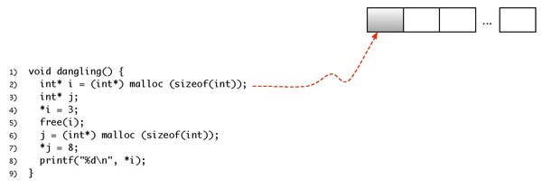
On line 3) we store a value into the block of memory used by i. The figure below shows it.

After storing a value into the block of memory used by i we release the space it was using. The figure below shows this situation.
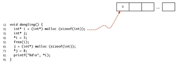
Notice that i still points to the block, that is, i still contains the address of that block. Also, the value previously stored in it is still there.
Now, let's stop for a bit and think of what happens on line 6). First, assume we are using a first fit strategy to allocate variables in the heap. From that assumption, as the first block of memory (the one previously used by i) is free, we can allocate j on it. And that's what happens, as we show below.
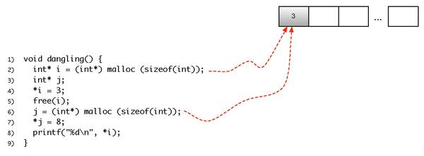
Now a different value is stored into the block of memory pointed by j:

Finally, on line 8) we print i. Commom sense tells us that 3 or possibly another value would be printed, but now we are able to tell why the value printed is actually 8.
Garbage Collection
Garbage collection
editGarbage collection (GC) is a form of automatic memory management. The garbage collector, or just collector, attempts to reclaim garbage, or memory occupied by objects that are no longer in use by the program. Garbage collection is often portrayed as the opposite of manual memory management, which requires the programmer to specify which objects to deallocate and return to the memory system. Garbage collection, like other memory management techniques, may take a significant proportion of total processing time in a program and can thus have significant influence on performance.
In this section we will describe three forms of Garbage Collection.
Mark and sweep
edit
A Mark and Sweep collector tries to find the live heap links and mark those blocks that are reachable. Then it makes a pass over the heap and returns unmarked free blocks to the free pool.
The mark-and-sweep method is the first known strategy for garbage collection. In this method, the garbage collector scans the program, starting from a point called root set (a set of objects easily identified in the program) and tries to reach other objects from then. The collector repeats this scanning until it cannot find any more reachable objects. Every time an object is found, its "being used" bit is set. After the collector finishes marking objects, it goes through the whole heap freeing those objects that do not have the "being used" bit set.
This method has several disadvantages, the most notable being that the entire system must be suspended during collection. This will cause programs to 'freeze' periodically (and generally unpredictably), making real-time and time-critical applications impossible.
Copying collection
editIn a Copying Collection collector memory is divided in two; only one half is used at a time. When used half is full, copy used blocks to the other location, and erase the old one.
This method has two big disadvantages. First, it has to stop the program's execution to move objects from one part of the heap to another. Second, it has to change the addresses to which program objects point to. This involves changing the values of variables in the program. In languages like C you store an object's address in an integer, making even harder for the garbage collector to find out which program variables store objects' addresses.
The biggest advantage of Copying Collection is the fact that if the size of the memory used by the program is less than the size of the half of the heap that is being used, no copying will be necessary, thus avoiding stopping the program and changing objects' addresses.
Reference counting
editIn a Reference Counting collector each block has a counter of heap links to it. This counter is incremented when a heap link is copied, decremented when the link is discarded. When the counter goes to zero, the block is freed. Compared to tracing garbage collection, reference counting guarantees that objects are destroyed as soon as they become unreachable.
The biggest advantage of Reference Counting is the fact that the program does not need to stop in order to perform garbage collection.The biggest disadvantages are:
- Extra space is used to store the reference counter.
- If two or more objects refer to each other, they can create a cycle where neither will be collected as their mutual references never let their reference counts become zero.
Parameter Matching
Virtually every programming languages provides developers with the capacity to build small pieces of code that can be activated from different parts of the program. This abstraction has different names in different languages. Just to name a few examples, Haskell provides functions. C, in addition to functions, provides procedures, which are functions that do not return values. Java and C# provides methods. Prolog provides inference rules. For simplicity, in this chapter we call all these abstraction functions. In every case, the calling code must pass parameters to the called code. There are many different ways to pass these parameters, and these policies are the subject of this chapter.
Parameter Matching
editMany authors name the parameters used in the declaration of the functions as formal parameters. As an example, the function div, below, written in python, has two formal parameters, dividend and divisor:
def div(dividend, divisor):
  r = dividend / divisor
  print "Result = ", r
When the function is called, we pass to it the so called actual parameters. For instance, in the code snippet below, we are passing to our function div two parameters, the variable x, and the constant 2.0:
>>> x = 3.0
>>> print div(x, 2.0)
Result =  1.5
In this example, the value stored in the variable x, the actual parameter, is used to initialize the value of divident, the formal parameter. In this case, the matching between formal and actual parameters is positional. In other words, actual parameters are matched with formal parameters based on the order in which they appear in the function call. Although the positional method is the usual way to match formal and actual parameters, there is another approach: the nominal matching.
>>> x = 3.0
>>> div(divisor=2.0, dividend=x)
Result =  1.5
This time, we explicitly name the actual parameter matched with the formal parameter. Nominal matching is present in a few programming languages, including ADA.
Parameters with Default Values
editSome programming languages give the developer the possibility to assign default values to parameters. For instance, Lets consider the same python function div seen before, but this time with a slightly different implementation:
def div(dividend=1.0, divisor=1.0):
   r = dividend / divisor
   print "Result = ", r
Each formal parameter, in this example, is assigned a default value. If the actual parameter that corresponds to that formal parameter is not present, the default value will be used. All the calls below are possible:
>>> div()
Result =  1.0
>>> div(dividend=3.2, divisor=2.3)
Result =  1.39130434783
>>> div(3.0, 1.5)
Result =  2.0
>>> div(3.0)
Result =  3.0
>>> div(1.5, divisor=3.0)
Result =  0.5
There are many languages that use default values. C++ is a well-known example in this family. All the calls below, for instance, give back valid answers. If the number of actual parameters is less than the number of formal parameters, then the default values are used. The matching, in this case, happens from the leftmost declaration towards the rightmost declaration. So, default values are applied to the formal paramters from the rightmost declaration to the leftmost.
#include <iostream>
class Mult {
  public:
    int f(int a = 1, int b = 2, int c = 3) const {
      return a * b * c;
    }
};
int main(int argc, char** argv) {
  Mult m;
  std::cout << m.f(4, 5, 6) << std::endl;
  std::cout << m.f(4, 5) << std::endl;
  std::cout << m.f(5) << std::endl;
  std::cout << m.f() << std::endl;
}
Functions with variable number of arguments
editThere are programming languages that let the developer to create functions with a variable number of arguments. The most well-known example is C, and the canonical example in this language is the printf function. This procedure receives as input a string describing the output that will be produced. By analyzing this string, the implementation of the printf function "knows" which are the next parameters that it probably will receive. Probably, because there is nothing in the C compiler that forces the developer to pass the right number of parameters and use the right types. The program below, for instance, is very likely to cause a runtime error due to a segmentation fault.
#include "stdio.h"
int main(int argc, char **argv) {
  printf("%s\n", argc);
}
The language C provides developers with a special syntax, and some library functions that let them create functions with a variable number of parameters. For instance, the function below is a function that can sum up four or less integer numbers. The first parameter is expected to be the number of arguments that the function must expect. The variable ap, is a data structure that points to each argument, as passed to the function foo. Inside the loop, we use the macro va_arg to obtain a pointer to each parameter. These pointers are stored in the array arr. Notice that va_arg is an example of how parametric polymorphism can be simulated in C. This language does not have type constructors, that is, it is not possible to pass a type to a function. However, we can simulate this capacity via macros.
#include <stdio.h>
#include <stdarg.h>

int foo(size_t nargs, ...) {
  int a = 0, b = 0, c = 0, d = 0;
  int *arr[4];
  va_list ap;
  size_t i;
  arr[0] = &a;
  arr[1] = &b;
  arr[2] = &c;
  arr[3] = &d;
  va_start(ap, nargs);
  for(i = 0; i < nargs; i++) {
    *arr[i] = va_arg(ap, int);
  }
  va_end(ap);
  return a + b + c + d;
}

int main() {
  printf("%d\n", foo(0));
  printf("%d\n", foo(1, 2));
  printf("%d\n", foo(2, 2, 3));
  printf("%d\n", foo(3, 2, 3, 5));
}
Again, there are no guarantees that the correct number of arguments will be passed to foo. As an example, the program below will print the value 10. The answer for this behavior is on the binary representation of the variable u. This variable occupies 8 bytes in memory, and each half is seen as a parameter.
int main() {
  // 10,00000000000000000000000000000011
  unsigned long long int u = 8589934595;
  printf("%d\n", foo(2, 5, u));
}
Evaluation Strategies
Evaluation Strategies
editThe parameter evaluation strategy adopted by a programming language defines when parameters are evaluated during function calls. There are two main strategies: strict and lazy evaluation.
Strict Evaluation
editThe strict evaluation strategy consists in the full evaluation of parameters before passing them to functions. The two most common evaluation strategies: by-value and by-reference, fit into this category.
Call-by-Value: The call-by-value strategy consists in copying the contents of the actual parameters into the formal parameters. State changes performed in the formal parameters do not reflect back into the actual parameters. A well-known example of this type of behavior is given by the swap function below, implemented in C:
void swap(int x, int y) {
  int aux = x;
  x = y;
  y = aux;;
}
int main() {
  int a = 2;
  int b = 3;
  printf("%d, %d\n", a, b);
  swap(a, b);
  printf("%d, %d\n", a, b);
}
Once the swap function is called, the contents of variables a and b are copied to the formal parameters x and y respectively. The data exchange that happens in the body of swap only affect the formal parameters, but not the actual ones. In other words, the swap call is innocuous in this program. In order to circumvent this semantics, the language C lets us use pointers to pass the address of a location, instead of its contents. Thus, the function below swaps the contents of two variables, as intended:
void swap(int *x, int *y) {
  int aux = *x;
  *x = *y;
  *y = aux;
}
int main() {
  int a = 2;
  int b = 3;
  printf("%d, %d\n", a, b);
  swap(&a, &b);
  printf("%d, %d\n", a, b);
}
The call-by-value strategy is very common among programming languages. It is the strategy of choice in C, Java, Python and even C++, although this last language also supports call-by-reference.
Call-by-Reference: whereas in the call-by-value strategy we copy the contents of the actual parameter to the formal parameter, in the call-by-reference we copy the address of the actual parameter to the formal one. A few languages implement the call-by-reference strategy. C++ is one of them. The program below re-implements the swap function, using the call-by-reference policy:
void swap(int &x, int &y) {
  int aux = x;
  x = y;
  y = aux;
}
int main() {
  int a = 2;
  int b = 3;
  printf("%d, %d\n", a, b);
  swap(a, b);
  printf("%d, %d\n", a, b);
}
In C++, parameter passing by reference is a syntactic sugar for the use of pointers. If we take a careful look into the assembly code that g++, the C++ compiler, produces for the function swap, above, and the function swap with pointers, we will realize that it is absolutely the same.
The call-by-reference might be faster than the call-by-value if the data-structures passed to the function have a large size. Nevertheless, this strategy is not present in the currently main-stream languages, but C++. Parameter passing by reference might lead to programs that are difficult to understand. For instance, the function below also implements the swap function; however, it combines three xor operations to avoid the need for an auxiliary variable.
void xor_swap(int &x, int &y) {
  x = x ^ y;
  y = x ^ y;
  x = x ^ y;
}
This function might lead to unexpected results if the formal parameters x and y alias the same location. For instance, the program below, which uses the xor_swap implementation zeros the actual parameter, instead of keeping its value:
int main() {
  int a = 2;
  int b = 3;
  printf("%d, %d\n", a, b);
  xor_swap(a, a);
  printf("%d, %d\n", a, b);
}
Lazy Evaluation
editThe strict evaluation strategies force the evaluation of the actual parameters before passing them to the called function. To illustrate this fact, the program below, implemented in python, loops.
def andF(a, b):
  if not a:
    return True
  else:
    return b

def g(x):
  if g(x):
    return True
  else:
    return False

f = andF(False, g(3))
There are parameter passing strategies that do not require the parameters to be evaluated before being passed to the called function. These strategies are called lazy. The three most well-known lazy strategies are call by macro expansion, call by name and call by need.
Call by Macro Expansion: many programming languages, including C, lisp and scheme, provide developers with a mechanism to add new syntax to the core language grammar called macros. Macros are expanded into code by a macro preprocessor. These macros might contain arguments, which are copied in the final code that the preprocessor produces. As an example, the C program below implements the swap function via a macro:
#define SWAP(X,Y) {int temp=X; X=Y; Y=temp;}
int main() {
  int a = 2;
  int b = 3;
  printf("%d, %d\n", a, b);
  SWAP(a, b);
  printf("%d, %d\n", a, b);
}
This macro implements a valid swap routine. The preprocessed program will look like the code below. Because the body of the macro is directly copied into the text of the calling program, it operates on the context of that program. In other words, the macro will refer directly to the variable names that it receives, and not to their values.
int main() {
  int a = 2;
  int b = 3;
  printf("%d, %d\n", a, b);
  { int tmp = (a); (a) = (b); (b) = tmp; };
  printf("%d, %d\n", a, b);
}
The expressions passed to the macro as parameters are evaluated every time they are used in the body of the macro. If the argument is never used, then it is simply not evaluated. As an example, the program below will increment the variable b twice:
#define MAX(X, Y) ((X) > (Y) ? (X) : (Y))
int main() {
  int a = 2, b = 3;
  int c = MAX(a, b++);
  printf("a = %d, b = %d, c = %d\n", a, b, c);
}
Macros suffer from one problem, called variable capture. If a macro defines a variable v that is already defined in the environment of the caller, and v is passed to the macro as a parameter, the body of the macro will not be able to distinguish one occurrence of v from the other. For instance, the program below has a macro that defines a variable temp. The call inside main causes the variable temp defined inside this function to be captured by the definition inside the macro's body.
#define SWAP(X,Y) {int temp=X; X=Y; Y=temp;}
int main() {
  int a = 2;
  int temp = 17;
  printf("%d, temp = %d\n", a, temp);
  SWAP(a, temp);
  printf("%d, temp = %d\n", a, temp);
}
Once this program is expanded by the C preprocessor, we get the code below. This program fails to exchange the values of variables temp and a:
int main() {
  int a = 2;
  int temp = 17;
  printf("%d, temp = %d\n", a, temp);
  {int temp=a; a=temp; temp=temp;};
  printf("%d, temp = %d\n", a, temp);
}
There are a number of lazy evaluation strategies that avoid the variable capture problem. The two best known techniques are call-by-name and call-by-need.
Call by Name: in this evaluation strategy the actual parameter is only evaluated if used inside the function; however, this evaluation uses the context of the caller routine. For instance, in the example below, taken from Weber's book, we have a function g that returns the integer 6. Inside the function f, the first assignment, e.g., b = 5, stores 5 in variable i. The second assignment, b = a, reads the value of i, currently 5, and adds 1 to it. This value is then stored at i.
void f(by-name int a, by-name int b) {
  b=5;
  b=a;
}
int g() {
  int i = 3;
  f(i+1,i);
  return i;
}
Very few languages implement the call by name evaluation strategy. The most eminent among these languages is Algol. Simula, a direct descendent of Algol, also implements call by name, as we can see in this example. The call by name always causes the evaluation of the parameter, even if this parameter is used multiple times. This behavior might be wasteful in referentially transparent languages, because, in these languages variables are immutable. There is an evaluation strategy that goes around this problem: the call by need.
Call by Need: in this evaluation strategy, a parameter is evaluated only if it is used. However, once the first evaluation happens, its result is cached, so that further uses of the parameter do not require a re-evaluation. This mechanism provides the following three guarantees:
- The expression is only evaluated if the result is required by the calling function;
- The expression is only evaluated to the extent that is required by the calling function;
- The expression is never evaluated more than once, called applicative-order evaluation.
Haskell is a language notorious for using call by need. This evaluation strategy is a key feature that the language designers have used to keep Haskell a purely functional language. For instance, call by need lets the language to simulate the input channel as an infinite list, which must be evaluated only as much as data has been read. An an example, the program below computes the n-th term of the Fibonacci Sequence. Yet, the function fib, that generates this sequence, has no termination condition!
fib m n = m : (fib n (m+n))

getIt [] _ = 0
getIt (x:xs) 1 = x
getIt (x:xs) n = getIt xs (n-1)

getN n = getIt (fib 0 1) n
The getIt function expands the list produced by fib only as many times as it is necessary to read its n-th element. For instance, below we have a sequence of calls that compute the 4-th element of the Fibonacci sequence:
getIt (fib 0 1) 4
= getIt (0 : fib 1 1) 4

getIt (fib 1 1) 3
= getIt (1 : fib 1 2) 3

getIt (fib 1 2) 2
= getIt (1 : fib 2 3) 2

getIt (fib 2 3) 1
= getIt (2 : fib 3 5) 1
= 2
Introduction to Cost Models
Programming language constructs might have particular asymptotic complexities, which programmers should know, to produce efficient algorithms. In other words, even though an algorithm has some specific, well-known, computational cost, its implementation can have higher complexity, due to an implicit cost model that is part of that languages runtime environment. Furthermore, some programming languages miss features, what might complicate the implementation of efficient algorithms. For instance, it will be hard to implement Bucket Sort without random access data structures. These minutia concern an aspect of programming languages' implementation that we call cost models.
In this chapter we will look into four cost models. The first concerns the use of lists in programming languages that follow the Lisp model. The second cost model concerns the invocation of functions in languages that support recursion. After that, we look into Prolog's unification model, trying to reason about the factors that cause unification to be more or less efficient. Finally, we discuss languages that support arrays, which are random access data structures.
List Cost Model
A Cost Model for Functional Lists
editList is possibly the most well-known data structure in functional programming languages. A functional list provides users with two well known operations: head and tail. The former returns the first element of the list. The latter returns a reference to the tail of the list, that is, the sublist that contains every element of the original sequence, but the first. With only these two operations, we cannot have random access, i.e., the ability to read any element in list paying the same fee in time. To illustrate this point, let's consider the implementation of the predicate below, which lets us concatenate lists:
@([], L, L).
@([H|T], L, [H|Tt]) :- @(T, L, Tt).
This predicate is formed by two clauses. The first is clearly O(1), because it is always true. The second, on the other hand, involves recursion. The predicate will be invoked recursively once, for each element on the first list. Each recursive call performs an O(1) amount of computation. Thus, this predicate is linear on the number of elements of the first list. Notice that we are talking about the number of elements, not the size of the elements. In other words, regardless of what the first list contains, the predicate should run always on the same time. As another example, let's this time analyze a naive implementation of a predicate to reverse lists:
reverse([],[]).
reverse([Head|Tail],Rev) :-  reverse(Tail,TailRev),  @(TailRev,[Head],Rev).
One could be tempted to believe that this predicate is linear on the size of the list that we want to invert: the first clause runs in O(1), and the second calls reverse once, recursively. However, the cost of each invocation of reverse is not O(1). Each of these calls, but the last, uses our append, which we already know to be O(N), N being the number of elements of the first list. Therefore, our current implementation of reverse is quadratic on the number of elements of the list. Given that is it so easy to invert an array in C, Python or Java in linear time, we could wonder if it is possible to achieve the same complexity on the cost model of functional lists. Indeed, that is possible, and we shall demonstrate it soon. For now, we shall push this question onto our stack.
Tail Call Cost Model
We start this section by recalling the implementation of reverse, which we discussed previously:
reverse_orig([],[]).
reverse_orig([Head|Tail],Rev) :-  reverse_orig(Tail,TailRev),  @(TailRev,[Head],Rev).
This implementation was quadratic on the number of elements of the list that we want to invert. Below, we have a different implementation, which is linear on the number of elements in the list that we want to invert:
reverse_opt(X,Y) :- rev(X,[],Y).
rev([],Sofar,Sofar).
rev([Head|Tail],Sofar,Rev) :-  rev(Tail,[Head|Sofar],Rev).
This predicate uses an auxiliary function, which has three arguments. The second among these arguments works as an accumulator: we are moving to the construction of the argument of the recursive call the tasks that before we were doing upon its return. This task, in our particular example, consists in adding an element to the beginning of the current version of the inverted list. It is easy to know that rev runs in linear time on the number of elements of the first list. This predicate has two clauses. The first, the base case, is O(1). The second, the inductive case, performs one recursive call, and the cost of each call is O(1), i.e., it consists in adding an element to the beginning of a list. Additionally, this predicate has another advantage, which we illustrate in w:gprolog:
| ?- length(L, 10000), reverse_opt(L, X).

L = [A,B ... ]

(354 ms) yes
| ?- length(L, 10000), reverse_orig(L, X).

Fatal Error: global stack overflow (size: 32768 Kb, environment variable used: GLOBALSZ)
So, what happened? The first version of reverse does not even terminates for large lists, whereas the second not only terminates just fine, but also runs very fast. The secret in this case is an optimization called Tail Call. If the last action of a function is to perform a recursive call, then the activation record of this function can be reused to store the new data. In other words, no new activation record is being created; there is only reuse of memory space going on. Effectively, this optimization transforms a recursive function into a C-style while loop. In principle, any recursive function can be optimized in this way. As an example, we show two functions, this time in SML, which are not tail-call, and show the corresponding tail call version:
fun sum [] = 0
  | sum (a::l) = sum l + a;

fun sum_opt thelist =
    let
      fun sum (nil, sofar) = sofar
      |   sum (head::tail, sofar) = sum (tail, sofar + head)
    in
      len (thelist, 0)
    end;

fun length nil = 0
|   length (head::tail) = 1 + length tail;

fun length_opt thelist =
    let
      fun len (nil, sofar) = sofar
      |   len (head::tail, sofar) = len (tail, sofar + 1)
    in
      len (thelist, 0)
    end;
The trick to transform the non-tail call function into a tail-call invocation is simple: create an auxiliary function that moves to the process of constructing the accumulator the computation that would be performed, otherwise, upon invocation return. As an example, SML's foldl implementation is tail call. The application of the folding operator happens during the construction of the new reduction seed, as we can see below:
fun foldl _ c nil = c
  | foldl f c (a::b) = foldl f (f(a,c)) b
Unification Cost Model
We start this section with a motivating question. What is the complexity of the predicate below, written in Prolog?
&=([], []).
&=([H|Tl], [H|Tr]) :- &=(Tl, Tr).
One could be easily tempted to say that this predicate is linear on the number of arguments of the smallest list. Yet, we could think about calls like:
&=([[1, 2, 3, 4, 5], [a, b, c, d, e]], [[1, 2, 3, 4, 5], [a, b, c, d, e]]).
We cannot solve this call to &= with two operations only. It is necessary to compare, one by one, all the two sublists that make up the larger lists. In this case, the complexity of &= is proportional to the size of the lists, not the number of elements of the lists. Unification-based search algorithms must scan entire data-structures in order to infer properties about them. And this scanning operation is exhaustive: every single possible combination of valid clauses will be explored during the resolution of unification. This brings in an important point: for efficiency reasons, it is better to solve the most restrictive clauses first, leaving those that are more open for later. For instance, let's consider the following predicates:
parent(d, a).
parent(f, e).
parent(a, b).
parent(e, b).
parent(e, c).
male(a).
male(d).
Given these terms, what, among these two implementations, is the best?
grandfather_1(X,Y) :- parent(X,Z), parent(Z,Y), male(X).

grandfather_2(X,Y) :- male(X), parent(X,Z), parent(Z,Y).
The second predicate is more efficient. To see why, notice that there are two clauses that unify with male(X) in our database of predicates: male(a) and male(b). Thus, the search tree for grandfather_2 starts with two nodes. Each of these nodes, which unifies with parent(X, Y), can have up to two nodes only, either parent(a, b) or parent(d, a), for a and d are the only atoms that satisfy male(X).

Had we used grandfather_1, then the story would be different. Our search tree, this time, starts with five nodes, for parent(X, Z) unifies with five clauses. Each one of these nodes, in turn, span three new nodes. This search tree is much larger than that one that grandfather_1 produces; consequently, it also takes longer to build. The bottom line of this discussion is: even though the order of terms within a predicate should bear no implication on its correctness, this order is still relevant for efficiency reasons. More restrictive predicates should come first, for they are more effective in pruning the search tree that is explored during the unification process.

Array Cost Model
We say that a data-structure is random access if the cost to read (or update) any element that it stores is the same, regardless of its position. Functional lists are clearly not random access: reading the n-th element is O(n). Arrays in C or Java, on the other hand, are. There are other data-structures which are also random access, at least on the average, such as hash-tables. Henceforth, we shall focus on C-style arrays. The key to random access lay on the fact that an array is stored contiguously in memory. Thus, an access such as a[i], in an array of type T, can be translated to the expression *(a + i). The same principle works for multidimensional arrays as well. As another example, a[i][j] in a 2-dimensional array of M lines and N columns, in C, translates to: *(a + i*N + j). However, even when we restrict ourselves to arrays, it is still difficult to ensure the same access cost always. The culprit is something called locality. To explain what is locality, let's consider two loops:
#include <stdio.h>
int main(int argc, char** argv) {
  const int M = 5000;
  const int N = 1000;
  char m[M][N];
  int i, j;

  if (argc % 2) {
    // initializes the array, row major:
    for (i = 0; i < M; i++) {
      for (j = 0; j < N; j++) {
        m[i][j] = 1;
      }
    }
  } else {
    // initializes the array, column major:
    for (j = 0; j < N; j++) {
      for (i = 0; i < M; i++) {
        m[i][j] = 1;
      }
    }
  }

  return 0;
}
This program runs at different speeds, depending on which loops executes (on an Intel core i5 at 1.4GHz):
$> clang -O0 trixSpeed.c -o trixSpeed

$>  time ./trixSpeed a

real	0m0.073s
user	0m0.068s
sys	0m0.003s

$> time ./trixSpeed

real	0m0.025s
user	0m0.019s
sys	0m0.003s
So, what is going on with this example? The same number of operations is performed, regardless of which loop runs. However, the first loop is 3.5x faster. As mentioned before, the key feature playing a role in these results is locality. Modern general purpose computer architectures use a cache. The cache is divided in lines. Data is not brought from main memory into the cache in individual pieces. Instead, a whole line is brought at once. If a program can access multiple datum on the same line, then memory trips can be avoided. On the other hand, if data is accessed across different lines, then multiple trips to the main memory must be performed. These trips are expensive, and they account for most of the running cost of this example.
How should a program be implemented, so that it can benefit more from locality? The answer is: it depends on the programming language. C organizes data in a row-major scheme. This means that in a 2-dimensional array, data on the same line are placed next to each other in memory. However, data in the same column can be quite far away. Cells in the same column, but in adjacent lines, will be N elements apart, where N is the line size in the 2-dimensional array. On the other hand, there are programming languages that organize data in column-major order. An example is Fortran. In this case, it is more efficient to fix columns and vary lines, while traversing 2-dimensional arrays.
Simple Predicates
Prolog is a programming language built around the notion of symbols: an atom is a symbol. Hence, unless we bestow some particular semantics into symbols like '1', '2' and '+', they will be treated in the same way as 'a', '@hi' and 'dcc024'. To make this notion of symbol a bit more clear, let's consider the predicate below, which was designed with the intended purpose of computing the length of a list:
myLength([], 0).
myLength([_|Tail], Len) :- myLength(Tail, TailLen), Len = TailLen + 1.
Even though this predicate has a pretty obvious implementation, if we run it, then, unless we are familiar with Prolog, we should get some unexpected result. For instance, in swi-prolog we get the following:
?- myLength([a, b, c], X).
X = 0+1+1+1.
That is not quite what we wanted, was it? The point is that '0', '+' and '1' are just atoms for unification purposes. Consequently, '0 + 1' has no more meaning than 'a + b', as we can check in swi-prolog:
?- X = a + b.
X = a+b.

?- X = 0 + 1.
X = 0+1.
Of course, Prolog offers ways to understand '1' as the number that this symbol represents. Similarly, the language provides ways to interpret '+' as arithmetic addition. One such way is to use the keyword is. A term like X is 1 + 1 has the following semantics: the right side of the equation, in this case, '1 + 1' is evaluated using the traditional interpretation of addition, and the result is then unified with the variable 'X'. Given this new keyword, we can re-write the length predicate in the following way:
isLength([], 0).
isLength([_|Tail], Len) :- isLength(Tail, TailLen), Len is TailLen + 1.
Notice that this predicate is not a tail recursive function. To make it so, we could add a third parameter to it, following the technique that we saw in the last chapter:
tailLength([], Acc, Acc).
tailLength([_|Tail], Acc, Len) :- NewAcc is Acc + 1, tailLength(Tail, NewAcc, Len).
Using the keyword is we can write several simple predicates that work on lists. These predicates rely on the same principles seen earlier, when we looked into Functional Programming. We have a base case, that determines what must be done once we reach the empty list, and we have an inductive step, which deals with non-empty lists. For instance, below we have an implementation of the predicate sum, which adds up the elements in a list. For completeness, we show also its tail recursive version:
sum([],0).
sum([Head|Tail],X) :- sum(Tail,TailSum), X is Head + TailSum.

sumAcc([], Acc, Acc).
sumAcc([H|T], Acc, X) :- Aux is Acc + H, sumAcc(T, Aux, X).
sumTC(L, S) :- sumAcc(L, 0, S).
Below we have an implementation of the ever present factorial predicate. Notice that in this example we check if an expression encodes an integer. Prolog is a dynamically typed programming language. Thus, atoms are just atoms. In principle, they are not treated as any special type. This means that we can have lists of numbers and other symbols, e.g., [1, +, a], for instance.
fact(0, 1).
fact(1, 1).
fact(N, F) :- integer(N), N > 1, N1 is N - 1, fact(N1, F1), F is F1 * N.
In addition to the operator is, Prolog offers also the operator =:= to evaluate arithmetic expressions. The semantics of this operator is slightly different than the semantics of is. The term X =:= Y forces the evaluation of both, X and Y. The result of this evaluation is then unified. For instance:
?- 1 + 2 is 4 - 1.
false.

?- 1 + 2 =:= 4 - 1.
true.

?- X is 4 - 1.
X = 3.

?- X =:= 4 - 1.
ERROR: =:=/2: Arguments are not sufficiently instantiated
In the last query we got an error, because variable 'X' was not defined. We cannot evaluate an undefined variable for its arithmetic value. We would get the same error if that variable were the right side of an 'is' expression:
?- 1 is X.
ERROR: is/2: Arguments are not sufficiently instantiated
Below we have an implementation of a naive greatest common divisor algorithm, which uses the =:= operator. We say that this algorithm is naive because it converges slowly, as we are using subtraction to equal the input numbers.
gcd(X, Y, Z) :- X =:= Y, Z is X.
gcd(X, Y, Denom) :- X > Y, NewY is X - Y, gcd(Y, NewY, Denom).
gcd(X, Y, Denom) :- X < Y, gcd(Y, X, Denom).
The faster Euclidean Algorithm would use division and remainders to reach a result faster.
gcd(N1, N2, GCD) :- N1 < N2, euclid(N2, N1, GCD).
gcd(N1, N2, GCD) :- N2 > 0, N1 > N2, euclid(N1, N2, GCD).

euclid(N, 0, N).
euclid(N1, N2, GCD) :- N2 > 0, Q is N1 // N2, R is N1 - (N2 * Q), euclid(N2, R, GCD).
Exhaustive Searches
Even though Prolog is a general purpose programming language, it really shines when we have to deal with problems involving exhaustive search. Many problems are like this, i.e., the only way to find an exact solution is through a brute force search. Two techniques are key to implement simple and elegant searches. The first is a way to produce subsets from a set, which we implement as follows:
subSet([], []).
subSet([H|T], [H|R]) :- subSet(T, R).
subSet([_|T], R) :- subSet(T, R).
The second technique is a way to produce permutations of a sequence. There are several ways to implement this predicate. Below we find a simple implementation:
perm([], []).
perm(List, [H|Perm]) :- select(H, List, Rest), perm(Rest, Perm).
So, which kind of problems are nicely solved via exhaustive search? NP-complete problems, for one, are a good start. Perhaps the simplest NP-complete problem is the Subset Sum Problem, which we state as follows: given a set S, and an integer N, is there a subset L within S whose sum adds up to N? A solution to this problem, in Prolog, is given below:
intSum(L, N, S) :- subSet(L, S), sumList(S, N).
We are using two predicates that we had seen earlier: subSet and sumList. The beauty of this solution is its simplicity. The Prolog solution, indeed, is a statement of the problem, almost in plain English. We say that a programming language is high-level it it reduces the semantic gap between a problem and an implementation of the solution to that problem. For this particular example, a description of the solution of the subset sum problem is also the solution itself. This problem illustrate the elegant and expressiveness of logic programming languages, when it comes to solving problems that involve exhaustive searches.
Notice that even problems that admit efficient exact solution can be solved through exhaustive search. Such brute force solutions are usually not efficient; however, they are elegant and illustrate well the basic structure of the problem that we want to solve. As an example, consider this sorting algorithm below, implemented through exhaustive search, which uses the perm predicate seen above. A sorted version of a list is a permutation of its elements, which meets the following property: given any two contiguous elements in the sorted list, H1 and H2, we have that H1 is less than, or equal to H2:
isSorted([]).
isSorted([_]).
isSorted([H1,H2|T]) :- H1 =< H2, isSorted([H2|T]).

mysort(L, S) :- perm(L, S), isSorted(S).
Of course, we can write more useful predicates using exhaustive search. For instance, what if we want to discover if a certain string represents an anagram of any English word? Assume that we have a dictionary dic.txt, with the known words, separated by a dot. The implementation of this predicate, in Prolog, can be seen below:
file_to_list(FILE, LIST) :- see(FILE), inquire([], LIST), seen.

inquire(IN, OUT):-
  read(Data),
  (Data == end_of_file -> OUT = IN; atom_codes(Data, LData), inquire([LData|IN], OUT)).

find_anagram(Dic, A, S) :- file_to_list(Dic, L), perm(A, X), member(X, L), name(S, X).
Several of the terms in the program above are part of the swipl standard library, e.g., see, seen, read, atom_codes and name. These predicates are used either to handle input and output, or to transform atoms into lists (atom_codes), and atoms into strings (name). Notice how perm is used to find all the permutations of the input string. Some of these permutations might have an equivalent in the list that was built out of the input file. If that is the case, then we report that as a solution to our problem. To execute this predicate, assuming that we have a file called 'dic.txt' in the local directory, we can do:
?- find_anagram('dic.txt', "topa", S).
S = pato ;
S = atop ;
And, if we want to join all the solutions into a single list, Prolog gives us the predicate findall, which works as follows:
?- findall(S, find_anagram('dic.txt', "topa", S), Solutions).
Solutions = [pato, atop].
This predicate receives three arguments. The term findall(S, Q, L) will build a list L, using the patterns S that are produced upon solving the query Q. Every pattern S that is a possible solution of Q shall be inserted in the output list. As an example, let us consider the three queries below:
?- findall(S, intSum([2, 3, 5, 7, 9, 11], 25, S), Answers).
Answers = [[2, 3, 9, 11], [2, 5, 7, 11], [5, 9, 11]].

?- findall(S, perm([a, b, c], S), Answers).
Answers = [[a, b, c], [a, c, b], [b, a, c], [b, c, a], [c, a, b], [c, b, a]].

?- findall(S, subSet([0, 1, 2], S), Answers).
Answers = [[0, 1, 2], [0, 1], [0, 2], [0], [1, 2], [1], [2], []].
As a last example of exhaustive search, we use Prolog to find cliques in graphs. The problem of finding a clique of size N in a graph is NP-complete. Therefore, it is very unlikely that we can have an efficient solution to this problem. Yet, we can have a simple one, in Prolog. To represent a graph, we can use a set of predicates representing edges. For instance:
edge(a, b).
edge(a, c).
edge(b, c).
edge(c, d).
edge(c, e).
edge(b, d).
edge(b, e).
edge(e, f).
edge(b, f).
These predicates determine a directed graph. In case we do not need directions, then we can have a predicate that checks if either edge(X, Y) or edge(Y, X) is in our database of predicates:
linked(X, Y) :- edge(X, Y).
linked(X, Y) :- edge(Y, X).
From these definitions, it is easy to produce a predicate that determines if a list of nodes form a clique:
clique([]).
clique([_]).
clique([X1,X2|R]) :- linked(X1, X2), clique([X1|R]), clique([X2|R]).
Finally, what we really want is to know if we have a clique of size N in our graph. Given the predicates that we already have, producing this query is almost like writing it in straightforward English:
cliqueN(V, C, N) :- sublist(V, C), clique(C), length(C, N).
Quest for Meaning
Semantics is the field concerned about the definition of meaning of programming constructs. There are several different notations to define such meaning. A few examples include:
The three different techniques mentioned above provide the means to explain, in a formal way, what each syntactic element of a programming language does. By formal, we mean unambiguous and mechanizable. A definition is unambiguous if there is only one way in which it can be interpreted. It is mechanizable if we can write that definition in a machine; thus, obtaining an interpreter for the programming language.
Formalism is good for several reasons. The first is that it helps in understanding a programming language. The meaning of programs is not always obvious. Even experts struggle sometimes to understand the behavior of code. And two programs, implemented in different languages, yet very similar, can have different behaviors. For instance, let us consider the following program, implemented in C:
#include <stdio.h>
int main() {
  int x = 1;
  x += (x = 2);
  printf("x = %d\n", x);
}
This program prints x = 4. Now, lets take a look into another program, this time implemented in Java:
public class T {
  public static void main(String args[]) {
    int x = 1;
    x += (x = 2);
    System.out.println("x = " + x);
  }
}
This program prints x = 3. Surprising, isn't it? And, which program is wrong? The answer to this question is: none of them. They all do what it is expected they should do, according to their semantics. In C, the assignment x += (x = 2) is translated into something like x = (x = 2) + x. In Java, on the other hand, we get something more like tmp = x; x = 2; x = x + tmp.
We shall see how to use operational semantics to describe the meaning of a programming language. The operational semantics describes meaning via an abstract machine. An abstract machine is an interpreter, i.e., a machine. However, this machine is not made of bolts and wires. It is made of mathematics. That is where the abstract in the name comes from.
To build an abstract machine we need a data-structure to represent programs. We already know such a data-structure: it is called the syntax tree, which we produce during parsing. However, the syntax tree has many elements that do not contribute to the meaning of programs. For instance, the two semi-colon marks, in the C command x = 1; x = x + 1; do not bear much voice in the final value stored in x. In this case, the semi-colon is there to help the parser to identify the end of commands. Similarly, markers such as the parentheses in the expression x * (y + z) are already encoded in the structure of the syntax tree. We do not really need to keep track of these tokens when building an interpreter to the programming language. Therefore, when designing interpreters, we need something that we call the abstract syntax of programs. Differently than the concrete syntax, the abstract syntax contains only the essential elements to let an interpreter navigate throughout the structure of programs.
An Interpreter for ML
In order to introduce the main concepts related to Operational Semantics, we shall define an interpreter for a subset of ML, which is comprehensive enough to include the lambda-calculus. We start with a very simple language, whose concrete syntax is given below:
    <exp> ::= <exp> + <mulexp>
            | <mulexp>
 <mulexp> ::= <mulexp> * <rootexp>
            | <rootexp>
<rootexp> ::= ( <exp> )
            | <constant>
As we had explained before, much of this syntax is boilerplate. The essential structure of the language that we want to interpret is much simpler:
<ast> ::= plus(<ast>, <ast>)
| times(<ast>, <ast>)
| const (<const>)
We have three kinds of elements so far: nodes denoting addition, multiplication and numbers. To produce an interpreter for this language, we need to define the actions that shall be taken once each of these nodes is visited. We shall produce such an interpreter in prolog. Because we have three varieties of nodes, we need to define three kinds of actions:
val(plus(X,Y),Value) :- val(X, XValue), val(Y, YValue), Value is XValue + YValue.
val(times(X,Y),Value) :- val(X, XValue), val(Y, YValue), Value is XValue * YValue.
val(const(X),X).
Our language, at this point, can only describe arithmetic expressions. Thus, the meaning of a program is always a number. Our prolog interpreter lets us get back this meaning:
| ?- val(const(10000), N). N = 10000 (1 ms) yes | ?- val(plus(const(10000), const(20)), N). N = 10020
Notice that it is not uncommon for the meaning of a program to be only a value. In the lambda-calculus, every program is a value. In a purely functional programming language we also have this semantics. For instance, as we shall proceed in our developments, we will increase our language with more syntax. The meaning of our programs, which contain variables and functions, are just values, where a value can be a number or a function. Talking about variables, this is the next addition to our programming language. In this case, we need syntax to create let blocks, as we have in ML. For instance:
- let val x = 2 in x * x end ; val it = 4 : int - let val x = 2 in let val x = 3 in x * x end + x end ; val it = 11 : int
To add let blocks to our programming language, we need to expand its concrete syntax. The new grammar can be seen below:
<exp> ::= <exp> + <mulexp>
| <mulexp>
<mulexp> ::= <mulexp> * <rootexp>
| <rootexp>
<rootexp> ::= let val <variable> = <exp> in <exp> end
| ( <exp> )
| <variable>
| <constant>
In terms of abstract syntax, let blocks force us to create two new kinds of nodes. The first node represents the let construct itself. The second represents names, i.e., surrogate for values. This expanded abstract syntax can be seen below:
<ast> ::= plus (<ast>, <ast>)
| times (<ast>, <ast>)
| const (<const>)
| let (<name>, <ast>, <ast>)
| var (<name>)
We need to augment our interpreter with two new clauses, to understand variables and let blocks. One question that surfaces now is how to keep track of the values of variables. To accomplish this task, we need the support of an environment. The environment is a table, that binds variable names to the values that these names represent. Notice that we are not talking about mutable variables: once assigned, a variable will have the same value until no longer in scope. Our new version of the interpreter is given below:
val(plus(X, Y), Context, Value) :-
val(X, Context, XValue),
val(Y, Context, YValue),
Value is XValue + YValue.
val(times(X, Y), Context, Value) :-
val(X, Context, XValue),
val(Y, Context, YValue),
Value is XValue * YValue.
val(const(X), _, X).
val(var(X), Context, Value) :-
lookup(X, Context, Value).
val(let(X, Exp1, Exp2), Context, Value2) :-
val(Exp1, Context, Value1),
val(Exp2, [(X, Value1)|Context], Value2).
lookup(Variable, [(Variable, Value)|_], Value).
lookup(VarX, [(VarY, _)|Rest], Value) :-
VarX \= VarY,
lookup(VarX, Rest, Value).
This new implementation lets us create variables, which we store and consult via the lookup predicate. The new semantics emulates well the behavior of blocks: a let binding creates a new scope, which is valid only within this block. As an example, below we show an ML program, and its equivalent version, in our language:
let val y = 3 in val(let(y,const(3),
let val x = y * y in let(x, times(var(y), var(y)),
x * x times(var(x), var(x)))),
end nil, X).
end
Notice that we do have the block semantics. For instance, below we see an interpretation of the program let val x = 1 in let val x = 2 in x end + x end. This program produces the value 3, as it would be expected in ML:
| ?- val(let(x, const(1), plus(let(x, const(2), var(x)), var(x))), nil, V). V = 3 ? ;
We want now to push the interpreter a bit further, to give it the ability to understand functions, including high-order functions and closures. This new addition means that a value can now be a function. As an example, the following program, in ML, returns a function, which denotes its meaning: let val f = fn x => x + 1 in f end. Adding functions to our language is more complicated than adding variables, because this addition requires a number of steps. In particular, our new concrete syntax is given by the grammar below:
<exp> ::= fn <variable> => <exp>
| <addexp>
<addexp> ::= <addexp> + <mulexp>
| <mulexp>
<mulexp> ::= <mulexp> * <funexp>
| <funexp>
<funexp> ::= <funexp> <rootexp>
| <rootexp>
<rootexp> ::= let val <variable> = <exp> in <exp> end
| ( <exp> )
| <variable>
| <constant>
First, we need to be able to distinguish two types of values: functions and numbers. Because our programming language does not contain a type system, we shall use a "marker" to separate functions from numbers. Thus, we will append the atom fval to every value that is a function. Such values are formed by a pair: the argument and the body of the function. This is to say that every function in our programming language uses only one parameter. This is similar to what we find in ML, e.g., anonymous functions have exactly these two components: a formal parameter plus a body. Examples of anonymous functions include: fn x => x * x, fn x => (fn y => x + y) and fn x => 1. Our abstract syntax can be seen below:
<ast> ::= plus (<ast>, <ast>)
| times (<ast>, <ast>)
| const (<const>)
| let (<name>, <ast>, <ast>)
| var (<name>)
| fn (<name>, <ast>)
| apply (<ast>, <ast>)
We have a node apply, which denotes function application. Notice that this node receives a whole AST node, instead of a simple name that would denote a function. This is expected, as functions can be the outcome of expressions. For example, this is a valid program: (let val f = fn x => x + 1 in f end) 2. In this case, the left side of the application is the expression let val f = fn x => x + 1 in f end, which, once evaluated, will yield the function fn x => x + 1. The extended version of our interpreter is given below:
val(plus(X, Y), Context, Value) :-
val(X, Context, XValue),
val(Y, Context, YValue),
Value is XValue + YValue.
val(times(X, Y), Context, Value) :-
val(X, Context, XValue),
val(Y, Context, YValue),
Value is XValue * YValue.
val(const(X), _, X).
val(var(X), Context, Value) :-
lookup(X, Context, Value).
val(let(X, Exp1, Exp2), Context, Value2) :-
val(Exp1, Context, Value1),
val(Exp2, [bind(X, Value1) | Context], Value2).
val(fn(Formal, Body), _, fval(Formal, Body)).
val(apply(Function, Actual), Context, Value) :-
val(Function, Context, fval(Formal, Body)),
val(Actual, Context, ParamValue),
val(Body, [bind(Formal, ParamValue)|Context], Value).
lookup(Variable, [bind(Variable, Value)|_], Value).
lookup(VarX, [bind(VarY, _)|Rest], Value) :-
VarX \= VarY, lookup(VarX, Rest, Value).
This new interpreter is powerful enough to handle programs as complicated as the code below, which is implemented in SML:
let val x = 1 in
let val f = fn n => n + x in
let val x = 2 in
f 0
end
end
end
This program, once evaluated, gives us a rather unexpected result:
| ?- val(let(x, const(1), let(f, fn(n, plus(var(n), var(x))), let(x, const(2), apply(var(f), const(0))))), nil, X). X = 2
We would expect to get 1 in ML. However, our interpreter gives back the value 2. The answer for this difference is simple: our interpreter uses dynamic scoping, whereas ML uses static scoping. This is natural: it is usually easier to implement dynamic scope. That is one of the reasons why some of the earlier programming languages such as Lisp used dynamic scope. But, as we had discussed before, static scope has many advantages of its dynamic counterpart. One of these advantages is the fact that we can use a function as a black-box. In other words, definitions that happen outside the body of a function will not change this function's behavior. In our case, implementing static scope is not difficult: we need to save the context that existed when the function was created. This new version of our interpreter implements static scoping:
val(plus(X, Y), Context, Value) :-
val(X, Context, XValue),
val(Y, Context, YValue),
Value is XValue + YValue.
val(times(X, Y), Context, Value) :-
val(X, Context, XValue),
val(Y, Context, YValue),
Value is XValue * YValue.
val(const(X), _, X).
val(var(X), Context, Value) :-
lookup(X, Context, Value).
val(let(X, Exp1, Exp2), Context, Value2) :-
val(Exp1, Context, Value1),
val(Exp2, [bind(X, Value1) | Context], Value2).
val(fn(Formal, Body), Context, fval(Formal, Body, Context)).
val(apply(Function, Actual), Context, Value) :-
val(Function, Context, fval(Formal, Body, Nesting)),
val(Actual, Context, ParamValue),
val(Body, [bind(Formal, ParamValue)|Nesting], Value).
lookup(Variable, [bind(Variable, Value)|_], Value).
lookup(VarX, [bind(VarY, _)|Rest], Value) :-
VarX \= VarY, lookup(VarX, Rest, Value).
In this new version of our interpreter, functions are now represented as triples fval(Formal, Body, Context)). Two of the elements in this triple, Formal and Body, are like before: the function's argument and its body. The third element, Context, is the bindings that existed when the function was created. The implementation of apply has also changed. Instead of evaluating a function in the context in which said function is called, we evaluate it in the context in which it was created. With this new interpreter we get the same behavior as in SML:
| ?- val(let(x, const(1), let(f, fn(n, plus(var(n), var(x))), let(x, const(2), apply(var(f), const(0))))), nil, X). X = 1
Notice that these two last versions of the interpreter are powerful enough to handle closures, just like SML does. For instance, we can write this program below in our interpreter, and run it:
let
val f = fn x => let val g = fn y => y+x in g end
in
f 1 2
end
If we translate it into our new language, then we have the following program:
?- val(let(f,fn(x,let(g,fn(y,plus(var(y),var(x))), var(g))), apply(apply(var(f),const(1)),const(2))),nil, X). X = 3