Introduction to Inorganic Chemistry/Molecular Orbital Theory

Chapter 2: Molecular Orbital Theory

The lowest unoccupied molecular orbital of the carbon monoxide molecule is a π antibonding orbital that derives from the 2p orbitals of carbon (left) and oxygen (right)

Valence bond (VB) theory gave us a qualitative picture of chemical bonding, which was useful for predicting the shapes of molecules, bond strengths, etc. It fails to describe some bonding situations accurately because it ignores the wave nature of the electrons.

Molecular orbital (MO) theory has the potential to be more quantitative. With it we can also get a picture of where the electrons are in the molecule, as shown in the image at the right. This can help us understand patterns of bonding and reactivity that are otherwise difficult to explain.

Although MO theory in principle gives us a way to calculate the energies and wavefunctions of electrons in molecules very precisely, usually we settle for simplified models here too. These simple models do not give very accurate orbital and bond energies, but they do explain concepts such as resonance (e.g., in the ferrocene molecule) that are hard to represent otherwise. We can get more accurate energies from MO theory by computational "number crunching." Many commercial and open-source programs have been developed for accurately calculating the electronic structure of molecules and extended solids.

While MO theory is more correct than VB theory and can be very accurate in predicting the properties of molecules, it is also rather complicated even for fairly simple molecules. For example, you should have no trouble drawing the VB pictures for CO, NH₃, and benzene, but we will find that these are increasingly challenging with MO theory.

Learning goals for Chapter 2:

• Be able to construct molecular orbital diagrams for homonuclear diatomic, heteronuclear diatomic, homonuclear triatomic, and heteronuclear triatomic molecules.
• Understand and be able to articulate how molecular orbitals form – conceptually, visually, graphically, and (semi)mathematically.
• Interrelate bond order, bond length, and bond strength for diatomic and triatomic molecules, including neutral and ionized forms.
• Use molecular orbital theory to predict molecular geometry for simple triatomic systems
• Rationalize molecular structure for several specific systems in terms of orbital overlap and bonding.
• Understand the origin of aromaticity and anti-aromaticity in molecules with π-bonding.

  2.1 Constructing molecular orbitals from atomic orbitals

Molecular orbital theory involves solving (approximately) the Schrodinger equation for the electrons in a molecule. To review from Chapter 1, this is a differential equation in which the first and second terms on the right represent the kinetic and potential energies:

$E\psi =-{\frac {\hbar ^{2}}{2\mu }}\nabla ^{2}\psi +V\psi$

While the Schrodinger equation can be solved analytically for the hydrogen atom, the potential energy function V becomes more complicated - and the equation can then only be solved numerically - when there are many (mutually repulsive) electrons in a molecule. So as a first approximation we will assume that the s, p, d, f, etc. orbitals of the atoms that make up the molecule are good solutions to the Schrodinger equation. We can then allow these wavefunctions to interfere constructively and destructively as we bring the atoms together to make bonds. In this way, we use the atomic orbitals (AO) as our basis for constructing MO's.

LCAO-MO = linear combination of atomic orbitals. In physics, this is called this the tight binding approximation.

We have actually seen linear combinations of atomic orbitals before when we constructed hybrid orbitals in Chapter 1. The basic rules we developed for hybridization also apply here: orbitals are added with scalar coefficients (c) in such a way that the resulting orbitals are orthogonal and normalized. The difference is that in the MO case, the atomic orbitals come from different atoms.

The linear combination of atomic orbitals always gives back the same number of molecular orbitals. So if we start with two atomic orbitals (e.g., an s and a p_z orbital as shown in Fig. 2.1.1), we end up with two molecular orbitals.

Fig. 2.1.2. Different components of endothelial cells are stained by blue, green, and red fluorescent dyes. For each dye the color of emitted light corresponds to the energy given off when an electron drops from the LUMO to the HOMO of the molecule.

Molecular orbitals are also called wavefunctions (ψ), because they are solutions to the Schrödinger equation for the molecule. The atomic orbitals (also called basis functions) are labeled as φ's, for example, φ_1s and φ_3pz or simply as φ₁ and φ₂.

In principle, we need to solve the Schrödinger equation for all the orbitals in a molecule, and then fill them up with pairs of electrons as we do for the orbitals in atoms. In practice we are really interested only in the MOs that derive from the valence orbitals of the constituent atoms, because these are the orbitals that are involved in bonding. We are especially interested in the frontier orbitals, i.e., the highest occupied molecular orbital (the HOMO) and the lowest unoccupied molecular orbital (the LUMO). Filled orbitals that are much lower in energy (i.e., core orbitals) do not contribute to bonding, and empty orbitals at higher energy likewise do not contribute. Those orbitals are however important in photochemistry and spectroscopy, which involve electronic transitions from occupied to empty orbitals. The fluorescent dyes that stain the cells shown in Fig. 2.1.2 absorb light by promoting electrons in the HOMO to empty MOs and give off light when the electrons drop back down to their original energy levels.

As an example of the LCAO-MO approach we can construct two MO's (ψ₁ and ψ₂) of the HCl molecule from two AO's φ₁ and φ₂ (Fig. 2.1.1). To make these two linear combinations, we write:

$\psi _{1}=c_{1}\phi _{1}+c_{2}\phi _{2}$

and

$\psi _{2}=c_{1}\phi _{1}-c_{2}\phi _{2}$

The coefficients c₁ and c₂ will be equal (or nearly so) when the two AOs from which they are constructed are the same, e.g., when two hydrogen 1s orbitals combine to make bonding and antibonding MOs in H₂. They will be unequal when there is an energy difference between the AOs, for example when a hydrogen 1s orbital and a chlorine 3p orbital combine to make a polar H-Cl bond.

Nodes:

The wavefunctions φ and ψ are amplitudes that are related to the probability of finding the electron at some point in space. They have lobes with (+) or (-) signs, which we indicate by shading or color. Wherever the wavefunction changes sign we have a node.

A representation of the nodes of different wavefunctions

When atomic orbitals add in phase, we get constructive interference and a lower energy orbital. When they add out of phase, we get a node and the resulting orbital has higher energy. The lower energy MOs are bonding and higher energy MOs are antibonding.

Fig. 2.1.1. Sigma bonding and antibonding combinations of an s and p orbital

As you can see in Fig. 2.1.1, nodes in MOs result from destructive interference of (+) and (-) wavefunctions. Generally, the more nodes, the higher the energy of the orbital.

In Fig. 2.1.1 we have drawn a simplified picture of the Cl 3p_z orbital and the resulting MOs, leaving out the radial node. Recall that 2p orbitals have no radial nodes, 3p orbitals have one, as illustrated in Fig. 2.1.3. 4p orbitals have two radial nodes, and so on. The MOs we make by combining the AOs have these nodes too.

Fig. 2.1.3. Nodal structure of 2p and 3p orbitals

Normalization:

The bonding in hypervalent molecules is described in terms of hybrid orbitals derived from valence s,p, and d orbitals. For two, or a set of orbitals to be individually normalized, the integral over all space of those orbitals should be equal to 1. This condition is expressed mathematically by the following integral:

$\int \phi _{i}\phi _{i}^{*}\,\mathrm {d} \tau =1$

Here φ_i represents the individual atomic orbitals, dτ represents the integration over all space (dτ = dx dy dz), and φ_i* is the complex conjugate of φ_i.

We square the wave functions to get probabilities, which are always positve or zero. So if an electron is in orbital φ₁, the probability of finding it at point xyz is the square of φ₁(x,y,z). When multiplying two identical atomic orbitals (ϕ_i×ϕ_i), the squared term equals 1. Conversely, cross terms that result from multiplying different atomic orbitals (ϕ_i×ϕ_j, where i≠j) integrate to 0. This arises from the fact that s,p and d atomic orbitals are normalized and orthogonal. Once added, the total probability density adds up to the sum of the atomic basis orbitals. Note that for wavefunctions that are real, φ = φ*.

The total probability does not change when we combine AOs to make MOs, so for the simple case of combining φ₁ and φ₂ to make ψ₁ and ψ₂,

$\psi _{1}^{2}+\psi _{2}^{2}=\phi _{1}^{2}+\phi _{2}^{2}$

Orthogonality and Orthonormality:

Aside from being normalized, hybrid orbitals display orthogonality if the following condition is satisfied:

$\int \phi _{i}\phi _{j}\,\mathrm {d} \tau =0$ for i ≠ j

Orthonormal atomic orbitals (AOs) possess both previously discussed key properties: orthogonality, which ensures zero overlap between distinct orbitals, and normalization, signifying that the integral of each orbital's probability density over all space equals one.

Fig. 2.1.4. The wavefunctions of atomic orbitals decrease exponentially with distance. Orbital overlap is non-zero when two atoms are close together, as illustrated for 1s orbitals in the upper figure. The lower figure shows orbitals that are too far away to interact. In this case both S and β are close to zero.

Overlap integral:

The spatial overlap between two atomic orbitals φ₁ and φ₂ is described by the overlap integral S,

$S_{12}=\int \phi _{1}^{*}\phi _{2}\,\mathrm {d} \tau$

where the integration is over all space ($\mathrm {d} \tau =\mathrm {d} x\,\mathrm {d} y\,\mathrm {d} z$).

Energies of bonding and antibonding MOs:

The energies of bonding and antibonding orbitals depend strongly on the distance between atoms. This is illustrated in Fig. 2.1.5 for the hydrogen molecule, H₂. At very long distances, there is essentially no difference in energy between the in-phase and out-of-phase combinations of H 1s orbitals. As they get closer, the in-phase (bonding) combination drops in energy because electrons are shared between the two positively charged nuclei. The energy reaches a minimum at the equilibrium bond distance (0.74 Å) and then rises again as the nuclei get closer together. The antibonding combination has a node between the nuclei so its energy rises continuously as the atoms are brought together.

Fig. 2.1.5. Energy as a function of distance for the bonding and antibonding orbitals of the H₂ molecule

At the equilibrium bond distance, the energies of the bonding and antibonding molecular orbitals (ψ₁, ψ₂) are lower and higher, respectively, than the energies of the atomic basis orbitals φ₁ and φ₂. This is shown in Fig. 2.1.6 for the MO’s of the H₂ molecule.

Fig. 2.1.6. Molecular orbital energy diagram for the H₂ molecule

The energy of an electron in one of the atomic orbitals is α, the Coulomb integral.

$\alpha =\int \phi _{1}^{*}H\phi _{1}\,\mathrm {d} \tau =\int \phi _{2}^{*}H\phi _{2}\,\mathrm {d} \tau$

where H is the Hamiltonian operator. Essentially, α represents the ionization energy of an electron in atomic orbital φ₁ or φ₂.

The energy difference between an electron in the AO’s and the MO’s is determined by the exchange integral β,

$\beta =\int \phi _{1}^{*}H\phi _{2}\,\mathrm {d} \tau$

β is an important quantity, because it tells us about the bonding energy of the molecule, and also the difference in energy between bonding and antibonding orbitals. Calculating β is not straightforward for multi-electron molecules because we cannot solve the Schrödinger equation analytically for the wavefunctions. We can however make some approximations to calculate the energies and wavefunctions numerically. In the Hückel approximation, which can be used to obtain approximate solutions for π molecular orbitals in organic molecules, we simplify the math by taking S=0 and setting H=0 for any p-orbitals that are not adjacent to each other. The extended Hückel method, developed by Roald Hoffmann, and other semi-empirical methods can be used to rapidly obtain relative orbital energies, approximate wavefunctions, and degeneracies of molecular orbitals for a wide variety of molecules and extended solids. More sophisticated ab initio methods are now readily available in software packages and can be used to compute accurate orbital energies for molecules and solids.

We can get the coefficients c₁ and c₂ for the hydrogen molecule by applying the normalization criterion:

$\psi _{1}={\frac {1}{\sqrt {2}}}{\frac {\phi _{1}+\phi _{2}}{1+S}}\qquad {\text{(bonding orbital)}}$

and

$\psi _{2}={\frac {1}{\sqrt {2}}}{\frac {\phi _{1}-\phi _{2}}{1-S}}\qquad {\text{(antibonding orbital)}}$

In the case where S≈0, we can eliminate the 1-S terms and both coefficients become 1/√2

Note that the bonding orbital in the MO diagram of H₂ is stabilized by an energy β/(1+S) and the antibonding orbital is destabilized by β/(1-S). That is, the antibonding orbital goes up in energy more than the bonding orbital goes down. This means that H₂ (ψ₁²ψ₂⁰) is energetically more stable than two H atoms, but He₂ with four electrons (ψ₁²ψ₂²) is unstable relative to two He atoms.

Bond order: In any MO diagram, the bond order can be calculated as ½ ( # of bonding electrons - # of antibonding electrons). For H₂ the bond order is 1, and for He₂ the bond order is zero.

Bond strengths and bond lengths: When we count bonds using MO theory, we use the formula above to calculate the net bond order. This formula would imply that the H₂⁺ and H₂^- molecules each have a bond order of 1/2, since there is one net bonding electron. However, experimentally we find that the bond is much longer and weaker in H₂^- than in H₂⁺. The table below summarizes the bond strengths and bond lengths for molecules and ions that use only their 1s atomic orbitals to make σ and σ* molecular orbitals.

MO configurations, bond lengths, and bond strengths of diatomic molecules and ions

Molecule	# of electrons	MO configuration	net # of bonding electrons	Bond order	Bond length (Å)	Bond energy (kJ/mol)
H2+	1	σ1s1	1	1/2	1.07	256
H2	2	σ1s2	2	1	0.74	436
H2-	3	σ1s2σ*1s1	1	1/2	-	156
He2+	3	σ1s2σ*1s1	1	1/2	1.08	230
He2	4	σ1s2σ*1s2	0	0	-	-

The striking difference between the bond strengths in H₂⁺ and H₂^- arises from the fact that there is electron-electron repulsion in the three-electron H₂^- ion, whereas there is none in H₂⁺. We also observe that the bond is much stronger in the three-electron He₂⁺ ion than it is in H₂^-. In the case of He₂⁺, the attraction between the electrons and the positive charge of the He²⁺ cores compensates for electron-electron repulsion. The moral of the story is that the MO diagrams we draw (just like the atomic orbitals we drew from the Schrödinger equation) are calculated for one-electron atoms, but in real (multi-electron) atoms and molecules we must consider electron-electron repulsion when we estimate or calculate bond energies.

Heteronuclear case (e.g., HCl) - Polar bonds

Here we introduce an electronegativity difference between the two atoms making the chemical bond. The energy of an electron in the H 1s orbital is higher (it is easier to ionize) than the electron in the chlorine 3p_z orbital. This results in a larger energy difference between the resulting molecular orbitals ψ₁ and ψ₂, as shown in Fig. 2.1.7. The bigger the electronegativity difference between atomic orbitals (the larger Δα is) the more “φ₂ character” the bonding orbital has, i.e., the more it resembles the Cl 3p_z orbital in this case. This is consistent with the idea that H-Cl has a polar single bond: the two electrons reside in a bonding molecular orbital that is primarily localized on the Cl atom.

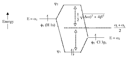
Fig. 2.1.7. Molecular orbital energy diagram for the HCl molecule

The antibonding orbital (empty) has more H-character. The bond order is again 1 because there are two electrons in the bonding orbital and none in the antibonding orbital.

Extreme case - Ionic bonding (NaF): very large Δα

In this case, there is not much mixing between the AO’s because their energies are far apart (Fig. 2.1.8). The two bonding electrons are localized on the F atom , so we can write the molecule as Na⁺F^-. Note that if we were to excite an electron from ψ₁ to ψ₂ using light, the resulting electronic configuration would be (ψ₁¹ψ₂¹) and we would have Na⁰F⁰. This is called a charge transfer transition.

Fig. 2.1.8. Molecular orbital energy diagram illustrating ionic bonding in the NaF molecule

Summary of molecular orbital theory so far:

• Add and subtract AO wavefunctions to make MOs. Two AOs → two MOs. More generally, the total number of MOs equals the number of AO basis orbitals.

• We showed the simplest case (only two basis orbitals). More accurate calculations use a much larger basis set (more AOs) and solve for the matrix of c’s that gives the lowest total energy, using mathematically friendly approximations of the potential energy function that is part of the Hamiltonian operator H.

• More nodes → higher energy MO

• Bond order = ½ ( # of bonding electrons - # of antibonding electrons)

• Bond polarity emerges in the MO picture as orbital “character.”

• AOs that are far apart in energy do not interact much when they combine to make MOs.

  2.2 Orbital symmetry

Fig. 2.2.1. Example of σ symmetry.

The MO picture for a molecule gets complicated when many valence AOs are involved. We can simplify the problem enormously by noting (without proof here) that orbitals of different symmetry with respect to the molecule do not interact. The symmetry operations of a molecule (which can include rotations, mirror planes, inversion centers, etc.), and the symmetry classes of bonds and orbitals in molecules, can be rigorously defined according to group theory. Here we will take a simple approach to this problem based on our intuitive understanding of the symmetry of three-dimensional objects as illustrated in Fig. 2.2.1.

AO’s must have the same nodal symmetry (as defined by the molecular symmetry operations), or their overlap is zero.

For example, in the HCl molecule, there is a unique symmetry axis →, which is typically defined as the Cartesian z-axis, as shown in Fig. 2.2.2.

Fig. 2.2.2. Orbitals of σ and π symmetry do not interact.

We can see from this figure that the H 1s orbital is unchanged by a 180° rotation about the bond axis. However, the same rotation inverts the sign of the Cl 3p_y wavefunction. Because these two orbitals have different symmetries, the Cl 3p_y orbital is nonbonding and doesn’t interact with the H 1s. The same is true of the Cl 3p_x orbital. The p_x and p_y orbitals have π symmetry (nodal plane containing the bonding axis) and are labeled π_nb in the MO energy level diagram, Fig. 2.2.3. In contrast, the H 1s and Cl 3p_z orbitals both have σ symmetry, which is also the symmetry of the clay pot shown in Fig. 2.2.1. Because these orbitals have the same symmetry (in the point group of the molecule), they can make the bonding and antibonding combinations shown in Fig. 2.1.1.

The MO diagram of HCl that includes all the valence orbitals of the Cl atom is shown in Fig. 2.2.3. Two of the Cl valence orbitals (3p_x and 3p_y) have the wrong symmetry to interact with the H 1s orbital. The Cl 3s orbital has the same (σ) symmetry as H 1s, but it is much lower in energy so there is little orbital interaction. The energy of the Cl 3s orbital is thus affected only slightly by forming the molecule. The pairs of electrons in the π_nb and σ_nb orbitals are therefore non-bonding.

Fig. 2.2.3. Energy level diagram of the HCl molecule showing MOs derived from the valence AOs.

Note that the MO result in Fig. 2.2.3 (1 bond and three pairs of nonbonding electrons) is the same as we would get from valence bond theory for HCl. The nonbonding orbitals are localized on the Cl atom, just as we would surmise from the valence bond picture.

In order to differentiate it from the σ bonding orbital, the σ antibonding orbital, which is empty in this case, is designated with an asterisk.

  2.3 σ, π, and δ orbitals

Fig. 2.3.1. The octachlorodirhenate(III) anion, [Re₂Cl₈]²⁻, which has a quadruple Re-Re bond.

Inorganic compounds use s, p, and d orbitals (and more rarely f orbitals) to make bonding and antibonding combinations. These combinations result in σ, π, and δ bonds (and antibonds).

You are already familiar with σ and π bonding in organic compounds. In inorganic chemistry, π bonds can be made from p- and/or d-orbitals. δ bonds are more rare and occur by face-to-face overlap of d-orbitals, as in the ion Re₂Cl₈^2-. The fact that the Cl atoms are eclipsed in this anion is evidence of δ bonding.

Some possible σ (top row), π (bottom row), and δ bonding combinations (right) of s, p, and d orbitals are sketched below. In each case, we can make bonding or antibonding combinations, depending on the signs of the AO wavefunctions. Because pπ-pπ bonding involves sideways overlap of p-orbitals, it is most commonly observed with second-row elements (C, N, O). π-bonded compounds of heavier elements are rare because the larger cores of the atoms prevent good π-overlap. For this reason, compounds containing C=C double bonds are very common, but those with Si=Si bonds are rare. δ bonds are generally quite weak compared to σ and π bonds. Compounds with metal-metal δ bonds occur in the middle of the transition series.

    

Transition metal d-orbitals can also form σ bonds, typically with s-p hybrid orbitals of appropriate symmetry on ligands. For example, phosphines (R₃P:) are good σ donors in complexes with transition metals, as shown at the right.

pπ-dπ bonding is also important in transition metal complexes. In metal carbonyl complexes such as Ni(CO)₄ and Mo(CO)₆, there is sideways overlap between filled metal d-orbitals and the empty π-antibonding orbitals (the LUMO) of the CO molecule, as shown in the figure at the left. This interaction strengthens the metal-carbon bond but weakens the carbon-oxygen bond. The C-O infrared stretching frequency is diagnostic of the strength of the bond and can be used to estimate the degree to which electrons are transferred from the metal d-orbital to the CO π-antibonding orbital.

The same kind of backbonding occurs with phosphine complexes, which have empty π orbitals, as shown at the right. Transition metal complexes containing halide ligands can also have significant pπ-dπ bonding, in which a filled pπ orbital on the ligand donates electron density to an unfilled metal dπ orbital. We will encounter these bonding situations in Chapter 5.

  2.4 Diatomic molecules

Valence bond theory fails for a number of the second row diatomics, most famously for O₂, where it predicts a diamagnetic, doubly bonded molecule with four lone pairs. O₂ does have a double bond, but it has two unpaired electrons in the ground state, a property that can be explained by the MO picture. We can construct the MO energy level diagrams for these molecules as follows:

                               Li₂, Be₂, B₂, C₂, N₂                                                         O₂, F₂, Ne₂

We get the simpler diatomic MO picture on the right when the 2s and 2p AOs are well separated in energy, as they are for O₂, F₂, and Ne₂. The picture on the left results from mixing of the σ_2s and σ_2p MO’s, which are close in energy for Li₂, Be₂, B₂, C₂, and N₂. The effect of this mixing is to push the σ_2s* down in energy and the σ_2p up, to the point where the pπ orbitals are below the σ_2p. Note that the energies of the π and π* orbitals are unaffected by s-p mixing because of symmetry considerations. The π and π* orbitals have "u" symmetry, meaning that they are antisymmetric with respect to the inversion operation. The σ and σ* orbitals orbitals have "g" symmetry, meaning that they are unchanged by inversion (see section 2.5). Heteronuclear diatomic molecules and ions such as CO, NO, and NO⁺ also have the ordering of energy levels shown on the left because of s-p mixing.

If you'd like to see what these bonding and antibonding molecular orbitals look like, a good animation of the MOs in the CO molecule can be found on the University of Liverpool Structure and Bonding website.

Why don't we get sp-orbital mixing for O₂ and F₂? The reason has to do with the energies of the orbitals, which are not drawn to scale in the simple picture at the left. As we move across the second row of the periodic table from Li to F, we are progressively adding protons to the nucleus. The 2s orbital, which has finite amplitude at the nucleus, "feels" the increased nuclear charge more than the 2p orbital. This means that as we progress across the periodic table (and also, as we will see later, when we move down the periodic table), the energy difference between the s and p orbitals becomes large compared to the bond energy. As the 2s and 2p energies become farther apart in energy, there is less interaction between the orbitals (i.e., less mixing).

A plot of orbital energies is shown at the right. Because of the very large energy difference between the 1s and 2s/2p orbitals, we plot them on different energy scales, with the 1s to the left and the 2s/2p to the right. For elements at the left side of the 2nd period (Li, Be, B) the 2s and 2p energies are only a few eV apart. The energy difference becomes very large - more than 20 electron volts (1930 kJ/mol) - for O and F. Since single bond energies are typically about 3-4 eV, this energy difference would be very large on the scale of our MO diagrams. For all the elements in the 2nd row of the periodic table, the 1s (core) orbitals are very low in energy compared to the 2s/2p (valence) orbitals, so we don't need to consider them in drawing our MO diagrams.

  2.5 Orbital filling

MO’s are filled from the bottom according to the Aufbau principle and Hund’s rule, as we learned for atomic orbitals.

Question: what is the quantum mechanical basis of Hund’s rule?

Consider the case of two degenerate orbitals, such as the π or π* orbitals in a second-row diatomic molecule. If these orbitals each contain one electron, their spins can be parallel (as preferred by Hund's rule) or antiparallel. The Pauli exclusion principle says that no two electrons in an orbital can have the same set of quantum numbers (n, l, m_l, m_s). That means that, in the parallel case, the Pauli principle prevents the electrons from ever visiting each other's orbitals. In the antiparallel case, they are free to come and go because they have different m_s quantum numbers. However, having two electrons in the same orbital is energetically unfavorable because like charges repel. Thus, the parallel arrangement, thanks to the Pauli principle, has lower energy.

For O₂ (12 valence electrons), we get the MO energy diagram below. The shapes of the molecular orbitals are shown at the right.

Oxygen molecular orbital diagram

Red giant stars are characterized by the presence of C₂ molecules in their atmospheres. Since C₂ has a net bond order of two, it reacts rapidly as it cools from the gas phase to make other forms of carbon such as fullerenes, graphite, and diamond, all of which have four bonds for every two carbon atoms.

This energy ordering of MOs correctly predicts two unpaired electrons in the π* orbital and a net bond order of two (8 bonding electrons and 4 antibonding electrons). This is consistent with the experimentally observed paramagnetism of the oxygen molecule.

Other interesting predictions of the MO theory for second-row diatomics are that the C₂ molecule has a bond order of 2 and that the B₂ molecule has two unpaired electrons (both verified experimentally).

We can also predict (using the O₂, F₂, Ne₂ diagram above) that NO has a bond order of 2.5, and CO has a bond order of 3.

The symbols "g" and "u" in the orbital labels, which we only include in the case of centrosymmetric molecules, refer to their symmetry with respect to inversion. Gerade (g) orbitals are symmetric, meaning that inversion through the center leaves the orbital unchanged. Ungerade (u) means that the sign of the orbital is reversed by the inversion operation. Because g and u orbitals have different symmetries, they have zero overlap with each other. As we will see below, factoring orbitals according to g and u symmetry simplifies the task of constructing molecular orbitals in more complicated molecules, such as butadiene and benzene.

The orbital shapes shown above were computed using a one-electron model of the molecule, as we did for hydrogen-like AOs to get the shapes of s, p, and d-orbitals. To get accurate MO energies and diagrams for multi-electron molecules (i.e. all real molecules), we must include the fact that electrons are “correlated,” i.e. that they avoid each other in molecules because of their negative charge. This problem cannot be solved analytically, and is solved approximately in numerical calculations by using density functional theory (DFT). We will learn about the consequences of electron correlation in solids (such as superconductors) in Chapter 10.

  2.6 Periodic trends in π bonding

As we noted in Section 2.3, pπ-bonding almost always involves a second-row element.

We encounter π-bonding from the sideways overlap of p-orbitals in the MO diagrams of second-row diatomics (B₂…O₂). It is important to remember that π-bonds are weaker than σ bonds made from the same AOs, and are especially weak if they involve elements beyond the second row.

Example:

comparison of ethylene and silylene structures

Ethylene: Stable molecule, doesn't polymerize without a catalyst.

Silylene: Never isolated, spontaneously polymerizes. Calculations indicate 117 kJ/mol stability in the gas phase relative to singly-bonded (triplet) H₂Si-SiH₂.

White phosphorus (P₄) is a soft, waxy solid that ignites spontaneously in air, burning with a bright flame and generating copious white P₄O₁₀ smoke. The sample shown here is photographed under water to prevent the oxidation reaction.

The large Ne core of Si atoms inhibits sideways overlap of 3p orbitals → weak π-bond.

Other examples: P₄ vs. N₂

comparison of elemental phosphorus and nitrogen structures

P cannot make π-bonds with itself, so it forms a tetrahedral molecule with substantial ring strain. This allotrope of P undergoes spontaneous combustion in air. Solid white phosphorus very slowly converts to red phosphorus, a more stable allotrope that contains sheets of pyramidal P atoms, each with bonds to three neighboring atoms and one lone pair.

N can make π-bonds, so N₂ has a very strong triple bond and is a relatively inert diatomic gas.

Silicone polymers (R₂SiO)_n are used in non-stick cookware like these muffin cups, in Silly Putty, soft robotics, and many other applications.

(CH₃)₂SiO vs. (CH₃)₂CO

comparison of polysiloxane and acetone structures

“RTV” silicone polymer (4 single bonds to Si) vs. acetone (C=O double bond). Silicones are soft, flexible polymers that can be heated to high temperatures (>300 °C) without decomposing. Acetone is a flammable molecular liquid that boils at 56 °C.


Also compare:
SiO₂ (mp ~1600°C) vs. CO₂ (sublimes at -78°C)

S₈ (solid, ring structure) vs. O₂ (gas, double bond)

Exceptions:

2nd row elements can form reasonably strong π-bonds with the smallest of the 3rd row elements, P, S, and Cl. Thus we find S=N bonds in sulfur-nitrogen compounds such as S₂N₂ and S₃N₃^-, P=O bonds in phosphoric acid and P₄O₁₀ (shown at the left), and a delocalized π-molecular orbital in SO₂ (as in ozone).

  2.7 Three-center bonding

Many (but not all) of the problems we will solve with MO theory derive from the MO diagram of the H₂ molecule (Fig. 2.1.5), which is a case of two-center bonding. The rest we will solve by analogy to the H₃⁺ ion, which introduces the concept of three-center bonding.

We can draw the H₃⁺ ion (and also H₃ and H₃^-) in either a linear or triangular geometry.

Walsh correlation diagram for H₃⁺:

walsh diagram for H3+

A few important points about this diagram:

• For the linear form of the ion, the highest and lowest MO’s are symmetric with respect to the inversion center in the molecule. Note that the central 1s orbital has g symmetry, so by symmetry it has zero overlap with the u combination of the two 1s orbitals on the ends. This makes the σ_u orbital a nonbonding orbital.

• In the triangular form of the molecule, the orbitals that derive from σ_u and σ*_g become degenerate (i.e., they have identically the same energy by symmetry). The term symbol “e” means doubly degenerate. We will see later that “t” means triply degenerate. Note that we drop the “g” and “u” for the triangular orbitals because a triangle does not have an inversion center.

• The triangular form is most stable because the two electrons in H₃⁺ have lower energy in the lowest orbital. Bending the molecule creates a third bonding interaction between the 1s orbitals on the ends.

MO diagram for XH₂ (X = Be, B, C…):

This is more complicated than H₃ because the X atom has both s and p orbitals. However, we can symmetry factor the orbitals and solve the problem by analogy to the H₂ molecule:

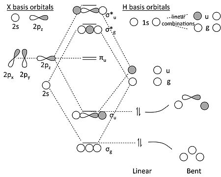
MO diagram for XH2

Some key points about this MO diagram:

• In the linear form of the molecule, which has inversion symmetry, the 2s and 2p orbitals of the X atom factor into three symmetry classes:

2s = σ_g

2p_z = σ_u

2p_x, 2p_y = π_u

• Similarly, we can see that the two H 1s orbitals make two linear combinations, one with σ_g symmetry and one with σ_u symmetry. They look like the bonding and antibonding MO’s of the H₂ molecule (which is why we say we use that problem to solve this one).

• The π_u orbitals must be non-bonding because there is no combination of the H 1s orbitals that has π_u symmetry.

• In the MO diagram, we make bonding and antibonding combinations of the σ_g’s and the σ_u’s. For BeH₂, we then populate the lowest two orbitals with the four valence electrons and discover (not surprisingly) that the molecule has two bonds and can be written H-Be-H. The correlation diagram shows that a bent form of the molecule should be less stable.

An interesting story about this MO diagram is that it is difficult to predict a priori whether CH₂ should be linear or bent. In 1970, Charles Bender and Henry Schaefer, using quantum chemical calculations, predicted that the ground state should be a bent triplet with an H-C-H angle of 135°. The best experiments at the time suggested that methylene was a linear singlet, and the theorists argued that the experimental result was wrong. Later experiments proved them right!

“A theory is something nobody believes, except the person who made it. An experiment is something everybody believes, except the person who made it.” – Einstein

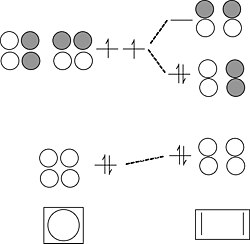
  2.8 Building up the MOs of more complex molecules: NH₃, P₄

MO diagram for NH₃

We can now attempt the MO diagram for NH₃, building on the result we obtained with triangular H₃⁺.

molecular orbital diagram for the ammonia molecule

Notes on the MO diagram for ammonia:

• Viewed end-on, a p-orbital or an sp_x hybrid orbital looks just like an s-orbital. Hence we can use the solutions we developed with s-orbitals (for H₃⁺) to set up the σ bonding and antibonding combinations of nitrogen sp³ orbitals with the H 1s orbitals.

• We now construct the sp³ hybrid orbitals of the nitrogen atom and orient them so that one is “up” and the other three form the triangular base of the tetrahedron. The latter three, by analogy to the H₃⁺ ion, transform as one totally symmetric orbital (“a₁”) and an e-symmetry pair. The hybrid orbital at the top of the tetrahedron also has a₁ symmetry.

• The three hydrogen 1s orbitals also make one a₁ and one (doubly degenerate) e combination. We make bonding and antibonding combinations with the nitrogen orbitals of the same symmetry. The remaining a₁ orbital on N is non-bonding. The dotted lines show the correlation between the basis orbitals of a₁ and e symmetry and the molecular orbitals

• The result in the 8-electron NH₃ molecule is three N-H bonds and one lone pair localized on N, the same as the valence bond picture (but much more work!).

P₄ molecule and P₄²⁺ ion:

By analogy to NH₃ we can construct the MO picture for one vertex of the P₄ tetrahedron, and then multiply the result by 4 to get the bonding picture for the molecule. An important difference is that there is relatively little s-p hybridization in P₄, so the lone pair orbitals have more s-character and are lower in energy than the bonding orbitals, which are primarily pσ.

P₄: 20 valence electrons

molecular orbital scheme for the P4 molecule

Take away 2 electrons to make P₄²⁺

Highest occupied MO is a bonding orbital → break one bond, 5 bonds left

Square form relieves ring strain, (60° → 90°)

structure of the P42+ion

2 π electrons

aromatic (4n + 2 rule)

  2.9 Homology of σ and π orbitals in MO diagrams

The ozone molecule (and related 18e molecules that contain three non-H atoms, such as NO₂^- and the allyl anion [CH₂-CH-CH₂]^-) is an example of 3-center 4-electron π-bonding. Our MO treatment of ozone is entirely analogous to the 4-electron H₃^- anion. We map that solution onto this one as follows:

constructing the ozone π-system by analogy to H3-

Professor Roald Hoffmann's ideas about orbital symmetry have helped explain the bonding and reactivity of organic and organometallic molecules, and also the structures and properties of extended solids.

The nonbonding π-orbital has a node at the central O atom. This means that the non-bonding electron pair in the π-system is shared by the two terminal O atoms, i.e., that the formal charge is shared by those atoms. This is consistent with the octet resonance structure of ozone.

This trick of mapping the solution for a set of s-orbitals onto a π-bonding problem is a simple example of a broader principle called the isolobal analogy. This idea, developed extensively by Roald Hoffmann at Cornell University, has been used to understand bonding and reactivity in organometallic compounds. In the isolobal analogy, symmetry principles (as illustrated above in the analogy between H₃^- and ozone) are used to construct MO diagrams of complex molecules containing d-frontier orbitals from simpler molecular fragments.


The triiodide ion. An analogous (and seemingly more complicated) case of 3-center 4-electron bonding is I₃^-. Each I atom has 4 valence orbitals (5s, 5p_x, 5p_y, 5p_z), making a total of 12 frontier orbitals, and the I₃^- anion has 22 electrons.

We can simplify the problem by recalling two periodic trends:

• The s-p orbital splitting is large, relative to the bond energy, after the second row of the periodic table. Thus, the 5s orbital is low in energy and too contracted to make bonds with its neighbors.
• π-overlap of 5p orbitals is very weak, so the 5p_x and 5p_y orbitals will also be non-bonding.
  

This leaves only the three 5p_z orbitals to make bonding/nonbonding/antibonding combinations. Again, the problem is entirely analogous to ozone or H₃^-.

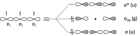
constructing the I3- MO diagram from frontier 5pz orbitals

Counting orbitals we obtain 9 lone pairs from the nonbonding 5s, 5p_x, and 5p_y orbitals, as well as one bond and one lone pair from the 5p_z orbital combinations above. The total of 10 nonbonding pairs and one bond accounts for the 22 electrons in the ion. The non-bonding 5p_z pair is localized on the terminal I atoms, giving each a -1/2 formal charge. This MO description is entirely consistent with the octet no-bond resonance picture of I₃^- that we developed in Chapter 1.

  2.10 Chains and rings of π-conjugated systems

ethylene molecule

        Ethylene: The π system is analogous to σ-bonding in H₂

homology of H2 and ethylene orbitals

Viewed from the top or bottom, the ethylene π-orbitals look like the H₂ σ orbitals. Thus we can map solutions from chains and rings of H atoms onto chains and rings of π-orbitals (as we did for the three-orbital case of O₃).

Chains and rings of four H atoms or π-orbitals (H₄ or butadiene):

MO diagram for H4 or butadiene

A few notes about this MO diagram:

• In the linear form of the molecule, the combination of AOs makes a ladder of evenly spaced energy levels that alternate g – u – g – u …. Each successive orbital has one more node. This is a general rule for linear chains of σ or π orbitals with even numbers of atoms.

• In the cyclic form of the molecule, there is one non-degenerate orbital at the bottom, one at the top, and a ladder of doubly degenerate orbitals in between. This is also a general rule for cyclic molecules with even numbers of atoms. This is the origin of the 4n+2 rule for aromatics.

• H₄ has four valence electrons, and by analogy butadiene has four π-electrons. These electrons fill the lowest two MOs in the linear form of the molecule, corresponding to two conjugated π-bonds in butadiene (H₂C=CH-CH=CH₂).

• In the cyclic form of the molecule, the degenerate orbitals are singly occupied. The molecule can break the degeneracy (and lower its energy) by distorting to a puckered rectangle. This is a general rule for anti-aromatic cyclic molecules (4n rule). Thus cyclobutadiene should be anti-aromatic and have two single and two double bonds that are not delocalized by resonance.

antiaromaticity of cyclobutadiene

Cyclobutadiene is actually a very unstable molecule because it polymerizes to relieve ring strain. Sterically hindered derivatives of the molecule do have the puckered rectangular structure predicted by MO theory.

Benzene π-orbitals:

How do we get from a 4-atom to 6-atom chain?

By analogy to the process we used to go from a 2-atom chain to a 4-atom chain, we now go from 4 to 6. We start with the orbitals of the 4-atom chain, which form a ladder of g and u orbitals. Then we make g and u combinations of the two atoms that we are adding at the ends. By combining g's with g's and u's with u's, we end up with the solutions for a string of 6 atoms. Closing these orbitals into a loop gives us the π molecular orbitals of the benzene molecule. The result is three π bonds, as we expected. Benzene fits the 4n+2 rule (n=2) and is therefore aromatic.

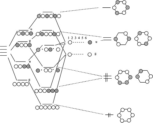
constructing the pi MOs of benzene

Here we have used the isolobal analogy to construct MO diagrams for π-bonded systems, such as ethylene and benzene, from combinations of s-orbitals. It raises the interesting question of whether the aromatic 4n+2 rule might apply to s-orbital systems, i.e., if three molecules of H₂ could get together to form an aromatic H₆ molecule. In fact, recent studies of hydrogen under ultra-high pressures in a diamond anvil cell show that such structures do form. A solid hydrogen phase exists that contains sheets of distorted six-membered rings, analogous to the fully connected 2D network of six-membered rings found in graphite or graphene. Anions with six π electrons in square four-membered rings are also aromatic. Examples are the dianion of cyclobutane, C₄H₄^2-, as well as the group 15 anions Bi₄^2-, Sb₄^2-, As₄^2-, and P₄^2-.

It should now be evident from our construction of MO diagrams for four- and six-orbital molecules that we can keep adding atomic orbitals to make chains and rings of 8, 10, 12... atoms. In each case, the g and u orbitals form a ladder of MOs. At the bottom rung of the ladder of an N-atom chain, there are no nodes in the MO, and we add one node for every rung until we get to the top, where there are N-1 nodes. Another way of saying this is that the wavelength of an electron in orbital x, counting from the bottom (1,2,3...x,...N), is 2Na/x, where a is the distance between atoms. We will find in Chapters 6 and 10 that we can learn a great deal about the electronic properties of metals and semiconductors from this model, using the infinite chain of atoms as a model for the crystal.

  2.11 Discussion questions

Ferrocene

• Derive the molecular orbital diagrams for linear and bent H₂O.
• Explain why the bond angles in H₂O and H₂S are different.
• We have derived the MO diagrams for the pi-systems of four- and six-carbon chains and rings. Repeat this exercise for a 5-carbon chain and 5-carbon ring (e.g., the cyclopentadienide anion), starting from the MO pictures for H₂ and H₃. This tricky problem helps us understand the electronic structure of ferrocene, and was the subject of a Nobel prize in 1973.

  2.12 Problems

1. The ionization energy of a hydrogen atom is 1312 kJ/mol and the bond dissociation energy of the H₂⁺ molecular ion is 256 kJ/mol. The overlap integral S for the H₂⁺ molecular ion is given by the expression S = (1 + R/a₀ + R²/3a₀²)exp(-R/a₀), where R is the bond distance (1.06 Å) and a₀ is the Bohr radius, 0.529 Å. What are the values of α and β (in units of kJ/mol) for H₂⁺?

2. Compare the bond order in H₂⁺ and H₂^- using the molecular orbital energy diagram for H₂. The bond dissociation energy of the H₂^- ion is 156 kJ/mol, while that for H₂⁺ is 256 kJ/mol. Is this what you would expect based on the bond orders? Why is the bond dissociation energy of H₂^- so much less than that of H₂⁺?

3. What is the bond order in HHe? Why has this compound never been isolated?

4. Would you expect the Be₂⁺ molecular ion to be stable in the gas phase? What is the total bond order, and how many net σ and π bonds are there?

5. Give a plausible explanation for the following periodic trend in F-X-F bond angles for gas-phase group 6 difluoride (XF₂) molecules. (Hint - it has something to do with a trend in s- and p-orbital energies; see Chapter 1, section 1.2)

Compound	F-M-F angle (degrees)
OF2	103
SF2	99
SeF2	97
TeF2	95

6. The most stable allotrope of oxygen is O₂, but the analogous sulfur molecule (S₂) is unstable relative to the S₈ allotrope. Explain why.

7. Using molecular orbital theory, show why the H₃ molecule has a triangular (or bent) rather than linear shape.

8. Use MO theory to determine the bond order and number of unpaired electrons in (a) O₂^-, (b) O₂⁺, (c) NO⁺, and (d) NO^-. Estimate the bond lengths in NO^- and NO⁺ using the Pauling formula and the bond length in the neutral NO molecule (1.151 Å).

10. Compare the results of MO theory and valence bond theory for describing the bonding in (a) CN^- and (b) neutral CN. According to MO theory, is it possible to have a bond order greater than 3 in a second-row diatomic molecule?

11. The neutral BN molecule is stable only in the gas phase. This molecule polymerizes to form solid boron nitride, which exists in both graphitic and ultra-hard diamond-like forms. Draw the molecular orbital energy diagram for the BN molecule. Determine the sigma and π bond orders and the number of unpaired electrons.

12. The bond distance in the gas phase BN molecule is 1.44 Å. Using the Pauling formula and the bond order you determined in Problem 11, calculate the B-N bond order in ammonia borane (H3B-NH3) where the bond distance is 1.658 Å. Does your calculation agree with expectated B-N bond order from valence bond theory?

13. Draw the MO diagram for the linear [FHF]^- ion. The only orbitals you need to worry about are the frontier orbitals, i.e., the H 1s and the two F sp_z hybrid orbitals that lie along the bonding (z) axis. What is the order of the HF bonds? What are the formal charges on the atoms?

14. The cyclooctatetraene (cot) molecule (picture a stop sign with four double bonds) has a puckered ring structure. However in U(cot)₂, where the oxidation state of uranium is 4+ and the cot ligand has a formal charge of 2-, the 8-membered rings are planar. Why is cot^2- planar?

15. Draw the following atomic orbitals, including different shading for different phases, the x, y, and z axes, and the name of the orbital.  Number them in order of energy, with the lowest energy orbital being #1, and increasing numbers as energy increases. Cutaway views are not necessary, just draw the surface. 3d_x2-y2, 2p_x, 3d_z2, 3s, 3p_y, 3d_xz, 3d_yz.

16. Draw the following molecular orbitals, including different shading for different phases, and the name of the orbital.  Number them in order of energy, with the lowest energy orbital being #1, and increasing numbers as energy increases. 1 σ_2p orbital, 2 different π*_2p orbitals, 1 σ*_2s orbital, 1 σ_1s orbital, 1 σ*_2p orbital.

17. Draw a Walsh diagram showing how the MO diagram changes going from a linear to a bent H-X-H molecule (where X is a second-row element such as Be, B, C, N, or O). Use this diagram to predict whether the H₂O molecule is linear or bent. Does the total bond order agree with the valence bond picture for H₂O ?