Introduction

OpenSCAD is software for creating solid 3D CAD objects.
It is free software and available for GNU/Linux, Microsoft Windows and Mac OS X.

Unlike most free software for creating 3D models (such as the well-known application Blender), OpenSCAD does not focus on the artistic aspects of 3D modelling, but instead focuses on the CAD aspects. So it might be the application you are looking for when you are planning to create 3D models of machine parts, but probably is not what you are looking for when you are more interested in creating computer-animated movies or organic life-like models.

OpenSCAD, unlike many CAD products, is not an interactive modeler. Instead it is something like a 2D/3D-compiler that reads in a program file that describes the object and renders the model from this file. This gives you (the designer) full control over the modelling process. This enables you to easily change any step in the modelling process and make designs that are defined by configurable parameters.

OpenSCAD has two main operating modes, Preview and Render. Preview is relatively fast using 3D graphics and the computer's GPU, but is an approximation of the model and can produce artifacts; Preview uses OpenCSG and OpenGL. Render generates exact geometry and a fully tessellated mesh. It is not an approximation and as such it is often a lengthy process, taking minutes or hours for larger designs. Render uses CGAL as its geometry engine.

OpenSCAD provides two types of 3D modelling:

Constructive Solid Geometry (CSG)
extrusion of 2D primitives into 3D space.

SVG is used for 2D while Autocad DXF files can be used as well for the data exchange format for 2D outlines. In addition to 2D paths for extrusion it is also possible to read design parameters from DXF files. Besides DXF files, OpenSCAD can read and create 3D models in the open 3mf, STL, OFF and many more file formats.

OpenSCAD can be downloaded from https://www.openscad.org/. More information is available on the mailing list.

Additional Resources

A clear guided introduction to using OpenSCAD and to the OpenSCAD language is available in the OpenSCAD Tutorial.

For Teachers: a basic 25-slide presentation from 2014 is available under GNUFDL to walk your students through the process of using OpenSCAD here.

Fablab Lannion (France) edited a nice French-language interactive tutorial that you might appreciate.

A "cheat sheet" is a useful quick reference for the OpenSCAD language, with each item linking back to this Wikibook.

A list of books can be found here.

History

Periodically the two manuals below get cleaned up or have major transitions. Consider archiving the manuals prior to starting a major update.

This can be done for the two 'printable version' links below to the Internet Archive

2018-04-25 The OpenSCAD User Manual - Print Version & The OpenSCAD Language - Print Version
2019-07-22 The OpenSCAD User Manual Which includes links to the archives of the above two printed versions (as of this date).

The Wayback Machine no longer has a free user requested site archive, so below is just the two 'printable version' manuals

2020-12-11 The OpenSCAD User Manual - Print Version & The OpenSCAD Language - Print Version

The OpenSCAD User Manual

A printable version of LABoyd2 is available. OpenSCAD_User_Manual (edit it)

Introduction
First Steps
The OpenSCAD User Interface
Input Devices
Customizer
Import - STL, 3MF, OFF, AMF, DXF, SVG, CSG
1. SVG Import
Export - STL, 3MF, OFF, AMF, DXF, SVG, CSG, PNG
Example Projects
1. Strandbeest
Paths
Using an external Editor with OpenSCAD
Integration with other applications
Using OpenSCAD in a command line environment
Building OpenSCAD from Sources
Frequently Asked Questions
Libraries
Tips and Tricks
Command Glossary - Very short name and syntax reference

The OpenSCAD Language Reference

A printable version of LABoyd2 is available. The_OpenSCAD_Language (edit it)

The OpenSCAD Language
1. General - READ THIS FIRST - comments, values and data types, variables, vectors, getting input
3D objects -
1. 3D Primitive Solids - cube, sphere, cylinder, polyhedron
2. 3D to 2D Projection
2D Objects
1. 2D Primitives - square, circle, polygon
2. Text - Generate text using installed or user supplied font files.
3. 2D to 3D - linear_extrude, rotate_extrude
Transform
1. color
2. rotate, translate, mirror, multmatrix
3. scale, resize
4. offset, minkowski, hull
5. Combining transformations
Boolean combination
1. union, difference, intersection, render
Other Functions and Operators
1. Conditional and Iterator Functions - for, intersection_for, if, conditional ? :, assign, let
2. Mathematical Operators - General, Vectors, Matrix multiplication
3. Mathematical Functions
  1. Trigonometric (cos sin tan acos asin atan atan2)
  2. Other (abs ceil concat cross exp floor ln len let log lookup max min norm pow rands round sign sqrt)
4. String Functions - str, chr, ord
5. Type Test Functions - is_undef, is_bool, is_num, is_string, is_list
6. List Comprehensions
7. Other Language Features - Special '$' variables, echo, render, surface, search , version(), version_num(), parent_module(n) and $parent_modules, assert
User-Defined Functions and Modules - Functions, Modules, Children
Debugging aids - % # ! * echo
External libraries and code files
1. include - SCAD, CSG
2. use - SCAD
3. import - STL, OFF, DXF
  1. import_dxf - Deprecated
  2. import_stl - Deprecated
4. export - STL, OFF, AMF, 3MF, DXF, SVG, PNG, CSG
5. surface - PNG

Work in progress

This section contains documentation about ongoing work which is available as experimental features in snapshot versions of OpenSCAD or not yet integrated at all and pending in a branch or pull-request at the OpenSCAD github repository.

Work in progress

Please add {{alphabetical}} only to book title pages.

First Steps

For our first model, we create a simple 2×3×4 cuboid.

To get started, launch OpenSCAD. You should have a preview window, toolbar, console and editor windows open. If one is hidden you can turn it on by going to the View menu and unselect the hidden items.

To create our cuboid we use the openSCAD editor window to type a one-line command:

	Usage example 1 - simple cuboid:

	cube([8,8,8]);

Compiling and rendering our first model

The cuboid can now be compiled and rendered by pressing F5 or F6 Function key on your keyboard while the OpenSCAD editor has focus. You should now see your object in the preview window as shown above.

Main Window of OpenSCAD with a small program generating the OpenSCAD-Logo.

The user interface of OpenSCAD has three parts

The viewing area
The console window
The text editor

Viewing area

Preview and rendering output goes into the viewing area. Using the Show Axes menu entry an indicator for the coordinate axes can be enabled.

Console window

Status information, warnings and errors are displayed in the console window.

During a render a progress-bar is displayed at the bottom of the console. It includes a Cancel button to stop the render.

A render can be cancel using the X button at the end of the progress bar.

Text editor

The built-in text editor provides basic editing features like text search & replace and also supports syntax highlighting. There are predefined color schemes that can be selected in the Preferences dialog.

OpenSCAD Editor with Find / Replace functionality.

Interactive modification of the numerical value

It is possible to change a numeric value in the source code and observe the result in real time.

Placing the cursor after a digit and pressing Alt+ up arrow or Alt + down arrow will increment or decrement the chosen digit. The object is re-rendered and displayed in preview mode after each change of the selected number in the source code. The cursor is moved after the next digit by Alt + right arrow, the further decimal digits are added when needed by moving the cursor after the last digit on the right side. The cursor is moved left behind the most significant digits of the number by Alt + left arrow.

NOTE: On MacOS, use Option + Shift instead of Alt.

Key	Description
`Alt` + `Up Arrow`	Increment the numeric value to the left of the cursor and preview the object.
`Alt` + `Down Arrow`	Decrement the numeric value to the left of the cursor and preview the object.
`Alt` + `Left Arrow`	Move the cursor left to more significant digit.
`Alt` + `Right Arrow`	Move the cursor right to less significant digit, eventually add one more decimal digit.

View navigation

The viewing area is navigated primarily using the mouse:

Action	Icons	Description
rotating the view		Dragging with the left mouse button rotates the view along the axes of the viewing area. It preserves the vertical axis' direction. Double-click the left button to set the point of rotation.
rotating the view	`⇧ Shift` +	Dragging with the left mouse button when the shift key is pressed rotates the view along the vertical axis and the axis pointing towards the user.
moving the viewing area		Dragging with the right mouse button moves the viewing area.
zooming		Using the scroll wheel
		Dragging with the middle mouse button
	`⇧ Shift` +	Dragging with the right or middle mouse button and the shift key pressed
	`⇧ Shift` +
	`+` and `-`	The keys `+` and `-`
show/hide rotation center	`Ctrl`+`3`	Turn on or off the graphic showing the center of rotation. (It is always in the center of the viewing area).
rotation reset	`Ctrl`+`0`	Rotation can be reset using the shortcut `Ctrl`+`0`.
translation reset	`Ctrl` + `⇧ Shift`+`0`	Translation can be reset using the shortcut `Ctrl`+`⇧ Shift`+`0`.

View setup

The viewing area can be configured to use different rendering methods and other options using the View menu. Most of the options described here are available using shortcuts as well.

Render modes

OpenCSG (F9)

This method produces instantaneous results, but has low frame rates when working with highly nonconvex objects.

Selecting the OpenCSG mode using F9 switches to the last generated OpenCSG view, but does not re-evaluate the source code. You may want to use the Compile function (F5, found in the Design menu) to re-evaluate the source code, build the OpenCSG objects and then switch to OpenCSG view.

Implementation Details

In OpenCSG mode, the OpenCSG library is used for generating the visible model. This library uses advanced OpenGL features (2.0) like the Z buffer and does not require an explicit description of the resulting mesh – instead, it tracks how objects are to be combined. For example, when rendering a spherical dent in a cube, it first renders the cube on the graphics card and then render the sphere, but instead of using the Z buffer to hide the parts of the sphere that are covered by the cube, it renders only those parts of the sphere, visually resulting in a cube with a spherical dent.

CGAL (Surfaces and Grid, F10 and F11)

This method might need some time when first used with a new program, but then has higher frame rates.

As before with OpenCSG, F10 and F11 enable only CGAL display mode and don't update the underlying objects; for that, use the Compile and Render function (F6, found in the Design menu).

To combine the benefits of those two display methods, you can selectively wrap parts of your program in a render function and force them to be baken into a mesh even with OpenCSG mode enabled.

Implementation Details

The acronym CGAL refers to The Open Source Computational Geometry Algorithms Library.

In CGAL mode, the CGAL library is used to compute the mesh of the root object, which is then displayed using simple OpenGL.

View options

Show Edges (Ctrl+1)

The difference between the CGAL and OpenCSG approaches can be seen at edges created by boolean operations.

If Show Edges is enabled, both OpenCSG and CGAL mode render edges as well as faces; CGAL even shows vertices. In CGAL grid mode, this option has no effect.

Enabling this option shows the difference between OpenCSG and CGAL quite clearly: While in CGAL mode you see an edge drawn everywhere it "belongs", OpenCSG does not show edges resulting from boolean operations – this is because they were never explicitly calculated but are just where one object's Z clipping begins or ends.

Show Axes (Ctrl+2)

If Show Axes is enabled, the origin of the global coordinate system is indicated by an orthogonal axes indicator. Additionally, a smaller axes indicator with axes names are shown in the lower left corner of the viewing area. The smaller axes indicator is marked x, y, z and coloured red, green, blue respectively.

Show Crosshairs (Ctrl+3)

If Show Crosshairs is enabled, the center of the viewport is indicated by four lines pointing in the room diagonal directions of the global coordinate system. This is useful when aligning the viewing area to a particular point in the model to keep it centered on screen during rotation.

Animation

The Animate option adds an animation bar to the lower edge of the screen. As soon as FPS and Steps are set (reasonable values to begin with are 10 and 100, respectively), the current Time is incremented by 1/Steps, FPS times per second, until it reaches 1, when it wraps back to 0.

Every time Time is changed, the program is re-evaluated with the variable $t set to the current time. Read more about how $t is used in section Other_Language_Features.

View alignment

The menu items Top, Bottom, …, Diagonal and Center (Ctrl+4, Ctrl+5, …, Ctrl+0, Ctrl+Shift+0) align the view to the global coordinate system.

Top, Bottom, Left, Right, Front and Back align it in parallel to the axes, the Diagonal option aligns it diagonally as it is aligned when OpenSCAD starts.

The Center option puts the coordinate center in the middle of the screen (but not rotate the view).

By default, the view is in Perspective mode, meaning that distances far away from the viewer appear shorter, as seen in the real world eyes or cameras. When the view mode is changed to Orthogonal, visible distances do not depend on the camera distance (the view simulates a camera at an infinite distance with an infinite focal length). This is especially useful in combination with the Top etc. options described above, as these orthogonal views result in a 2D images similar to what one would see in an engineering drawing.

The OpenSCAD Language

The text in its current form is incomplete.

OpenSCAD is a 2D/3D and solid modeling program that is based on a Functional programming language used to create models that are previewed on the screen, and rendered into 3D mesh which allows the model to be exported in a variety of 2D/3D file formats.

A script in the OpenSCAD language is used to create 2D or 3D models. This script is a free format list of action statements.

 object();
 variable = value;
 operator()   action();
 operator() { action();    action(); }
 operator()   operator() { action(); action(); }
 operator() { operator()   action();
              operator() { action(); action(); } }

Objects: Objects are the building blocks for models, created by 2D and 3D primitives. Objects end in a semicolon ';'.; Examples are: cube(), sphere(), polygon(), circle(), etc.

Actions: Action statements include creating objects using primitives and assigning values to variables. Action statements also end in a semicolon ';'.; Example: a=1; b = a+7;

Operators: Operators, or transformations, modify the location, color and other properties of objects. Operators use braces '{}' when their scope covers more than one action. More than one operator may be used for the same action or group of actions. Multiple operators are processed Right to Left, that is, the operator closest to the action is processed first. Operators do not end in semicolons ';', but the individual actions they contain do.; Examples:

   cube(5);
   x = 4+y;
   rotate(40) square(5,10);
   translate([10,5]) { circle(5); square(4); }
   rotate(60) color("red") { circle(5); square(4); }
   color("blue") { translate([5,3,0]) sphere(5); rotate([45,0,45]) { cylinder(10); cube([5,6,7]); } }

Comments

Comments are a way of leaving notes within the script, or code, (either to yourself or to future programmers) describing how the code works, or what it does. Comments are not evaluated by the compiler, and should not be used to describe self-evident code.

OpenSCAD uses C++-style comments:

// This is a comment
  
myvar = 10; // The rest of the line is a comment
  
/*
   Multi-line comments
   can span multiple lines.
*/

Values and data types

A value in OpenSCAD is either a Number (like 42), a Boolean (like true), a String (like "foo"), a Range (like [0: 1: 10]), a Vector (like [1,2,3]), or the Undefined value (undef). Values can be stored in variables, passed as function arguments, and returned as function results.

[OpenSCAD is a dynamically typed language with a fixed set of data types. There are no type names, and no user defined types.]

Numbers

Numbers are the most important type of value in OpenSCAD, and they are written in the familiar decimal notation used in other languages. Eg, -1, 42, 0.5, 2.99792458e+8. [OpenSCAD does not support octal or hexadecimal notation for numbers.]

In addition to decimal numerals, the following names for special numbers are defined:

PI

OpenSCAD has only a single kind of number, which is a 64 bit IEEE floating point number. OpenSCAD does not distinguish integers and floating point numbers as two different types, nor does it support complex numbers. Because OpenSCAD uses the IEEE floating point standard, there are a few deviations from the behaviour of numbers in mathematics:

We use binary floating point. A fractional number is not represented exactly unless the denominator is a power of 2. For example, 0.2 (2/10) does not have an exact internal representation, but 0.25 (1/4) and 0.125 (1/8) are represented exactly.
The largest representable number is about 1e308. If a numeric result is too large, then the result can be infinity (printed as inf by echo).
The smallest representable number is about -1e308. If a numeric result is too small, then the result can be -infinity (printed as -inf by echo).
If a numeric result is invalid, then the result can be Not A Number (printed as nan by echo).
If a non-zero numeric result is too close to zero to be representable, then the result is -0 if the result is negative, otherwise it is 0. Zero (0) and negative zero (-0) are treated as two distinct numbers by some of the math operations, and are printed differently by 'echo', although they compare as equal.

The constants inf and nan are not supported as numeric constants by OpenSCAD, even though you can compute numbers that are printed this way by 'echo'. You can define variables with these values by using:

inf = 1e200 * 1e200;
nan = 0 / 0;
echo(inf,nan);

The value nan is the only OpenSCAD value that is not equal to any other value, including itself. Although you can test if a variable 'x' has the undefined value using 'x == undef', you can't use 'x == 0/0' to test if x is Not A Number. Instead, you must use 'x != x' to test if x is nan.

Boolean values

Booleans are variables with two states, typically denoted in OpenSCAD as true and false. Boolean variables are typically generated by conditional tests and are employed by conditional statement 'if()'. conditional operator '? :', and generated by logical operators ! (not), && (and), and || (or). Statements such as if() actually accept non-boolean variables, but most values are converted to true in a boolean context. The values that count as false are:

false
0 and -0
""
[]
undef

Note that "false" (the string), [0] (a numeric vector), [ [] ] (a vector containing an empty vector), [false] (a vector containing the Boolean value false) and 0/0 (not a number) all count as true.

Strings

A string is a sequence of zero or more unicode characters. String values are used to specify file names when importing a file, and to display text for debugging purposes when using echo(). Strings can also be used with the text() primitive, added in version 2015.03.

A string literal is written as a sequence of characters enclosed in quotation marks ", like this: "" (an empty string), or "this is a string".

To include a " character in a string literal, use \". To include a \ character in a string literal, use \\. The following escape sequences beginning with \ can be used within string literals:

\" → "
\\ → \
\t → tab
\n → newline
\r → carriage return
\x21 → ! - only valid in the range from \x01 to \x7f, \x00 produces a space
\u03a9 → Ω - 4 digit unicode code point, see text() for further information on unicode characters
\U01f600 → 😀 - 6 digit unicode code point

This behavior is new since OpenSCAD-2011.04. You can upgrade old files using the following sed command: sed 's/\\/\\\\/g' non-escaped.scad > escaped.scad

Example:

 echo("The quick brown fox \tjumps \"over\" the lazy dog.\rThe quick brown fox.\nThe \\lazy\\ dog.");
  
 result

   ECHO: "The quick brown fox     jumps "over" the lazy dog.
   The quick brown fox.
   The \lazy\ dog."
  
 old result
   ECHO: "The quick brown fox \tjumps \"over\" the lazy dog.
   The quick brown fox.\nThe \\lazy\\ dog."

Ranges

Ranges are used by for() loops and children(). They have 2 varieties:

[<start>:<end>]

[<start>:<increment>:<end>]

Although enclosed in square brackets [] , they are not vectors. They use colons : for separators rather than commas.

r1 = [0:10];
r2 = [0.5:2.5:20];
echo(r1); // ECHO: [0: 1: 10]
echo(r2); // ECHO: [0.5: 2.5: 20]

You should avoid step values that cannot be represented exactly as binary floating point numbers. Integers are okay, as are fractional values whose denominator is a power of two. For example, 0.25 (1/4) and 0.125 (1/8) are safe, but 0.2 (2/10) should be avoided. The problem with these step values is that your range may have too many or too few elements, due to inexact arithmetic.

A missing <increment> defaults to 1. A range in the form [<start>:<end>] with <start> greater than <end> generates a warning and is equivalent to [<end>: 1: <start>]. A range in the form [<start>:1:<end>] with <start> greater than <end> does not generate a warning and is equivalent to []. The <increment> in a range may be negative (for versions after 2014).

The undefined value

The undefined value is a special value written as undef. It is the initial value of a variable that hasn't been assigned a value, and it is often returned as a result by functions or operations that are passed illegal arguments. Finally, undef can be used as a null value, equivalent to null or NULL in other programming languages.

All arithmetic expressions containing undef values evaluate as undef. In logical expressions, undef is equivalent to false. Relational operator expressions with undef evaluate as false except for undef==undef which is true.

Note that numeric operations may also return 'nan' (not-a-number) to indicate an illegal argument. For example, 0/false is undef, but 0/0 is 'nan'. Relational operators like < and > return false if passed illegal arguments. Although undef is a language value, 'nan' is not.

Variables

OpenSCAD variables are created by a statement with a name or identifier, assignment via an expression and a semicolon. The role of arrays, found in many imperative languages, is handled in OpenSCAD via vectors. Currently valid identifiers can only be composed of simple characters and underscores [a-zA-Z0-9_] and do not allow high-ascii or unicode characters.

var = 25;
xx = 1.25 * cos(50);
y = 2*xx+var;
logic = true;
MyString = "This is a string";
a_vector = [1,2,3];
rr = a_vector[2];      // member of vector
range1 = [-1.5:0.5:3]; // for() loop range
xx = [0:5];            // alternate for() loop range

OpenSCAD is a Functional programming language, as such variables are bound to expressions and keep a single value during their entire lifetime due to the requirements of referential transparency. In imperative languages, such as C, the same behavior is seen as constants, which are typically contrasted with normal variables.

In other words OpenSCAD variables are more like constants, but with an important difference. If variables are assigned a value multiple times, only the last assigned value is used in all places in the code. See further discussion at Variables are set at compile-time, not run-time. This behavior is due to the need to supply variable input on the command line, via the use of -D variable=value option. OpenSCAD currently places that assignment at the end of the source code, and thus must allow a variable's value to be changed for this purpose.

Values cannot be modified during run time; all variables are effectively constants that do not change. Each variable retains its last assigned value at compile time, in line with Functional programming languages. Unlike Imperative languages, such as C, OpenSCAD is not an iterative language, and as such the concept of x = x + 1 is not valid. Understanding this concept leads to understanding the beauty of OpenSCAD.

Before version 2015.03, it was not possible to do assignments at any place except the file top-level and module top-level. Inside an if/else or for loop, assign() was needed.

Since version 2015.03, variables can now be assigned in any scope. Note that assignments are only valid within the scope in that they are defined - you are still not allowed to leak values to an outer scope. See Scope of variables for more details.

a=0;
if (a==0) 
  {
 a=1; //  before 2015.03 this line would generate a Compile Error
      //  since 2015.03  no longer an error, but the value a=1 is confined to within the braces {}
  }

Undefined variable

A non assigned variable has the special value undef. It could be tested in conditional expression, and returned by a function.

 Example
  
 echo("Variable a is ", a);                // Variable a is undef
 if (a==undef) {
   echo("Variable a is tested undefined"); // Variable a is tested undefined
 }

Scope of variables

When operators such as translate() and color() need to encompass more than one action ( actions end in ;), braces {} are needed to group the actions, creating a new, inner scope. When there is only one semicolon, braces are usually optional.

Each pair of braces creates a new scope inside the scope where they were used. Since 2015.03, new variables can be created within this new scope. New values can be given to variables that were created in an outer scope. These variables and their values are also available to further inner scopes created within this scope, but are not available to anything outside this scope. Variables still have only the last value assigned within a scope.

                       // scope 1
 a = 6;                // create a
 echo(a,b);            //                6, undef
 translate([5,0,0]){   // scope 1.1
   a= 10;
   b= 16;              // create b
   echo(a,b);          //              100, 16   a=10; was overridden by later a=100;
   color("blue") {     // scope 1.1.1
     echo(a,b);        //              100, 20
     cube();
     b=20;
   }                   // back to 1.1
   echo(a,b);          //              100, 16
   a=100;              // override a in 1.1
 }                     // back to 1   
 echo(a,b);            //                6, undef
 color("red"){         // scope 1.2
   cube();
   echo(a,b);          //                6, undef
 }                     // back to 1
 echo(a,b);            //                6, undef
  
 //In this example, scopes 1 and 1.1 are outer scopes to 1.1.1 but 1.2 is not.

Anonymous scopes are not considered scopes:

 {
   angle = 45;
 }
 rotate(angle) square(10);

For() loops are not an exception to the rule about variables having only one value within a scope. A copy of loop contents is created for each pass. Each pass is given its own scope, allowing any variables to have unique values for that pass. No, you still can't do a=a+1;

Variables are set at compile-time, not run-time

Because OpenSCAD calculates its variable values at compile-time, not run-time, the last variable assignment within a scope applies everywhere in that scope or inner scopes thereof. It may be helpful to think of them as override-able constants rather than as variables.

// The value of 'a' reflects only the last set value
   a = 0;
   echo(a);  // 5
   a = 3;
   echo(a);  // 5
   a = 5;

While this appears to be counter-intuitive, it allows you to do some interesting things: for instance, if you set up your shared library files to have default values defined as variables at their root level, when you include that file in your own code you can 're-define' or override those constants by simply assigning a new value to them. So changing constant values gives you more flexibility. If constants would never change, of course, you always can be sure having the value you see in any constant definition. Not so here. If you see a constant value definition at any other place its value could be different. This is very flexible.

The preceding description appears to differ from the behaviour of OpenSCAD as at May 23 2022. At that date, running the above example causes the following output:

WARNING: a was assigned on line 1 of "Untitled" but was overwritten in file Untitled, line 3 Execution aborted

Special variables

Special variables provide an alternate means of passing arguments to modules and functions. All variables starting with a '$' are special variables, similar to special variables in lisp. As such they are more dynamic than regular variables. (for more details see Other Language Features)

Vectors

A vector or list is a sequence of zero or more OpenSCAD values. Vectors are collections of numeric or boolean values, variables, vectors, strings or any combination thereof. They can also be expressions which evaluate to one of these. Vectors handle the role of arrays found in many imperative languages. The information here also applies to lists and tables which use vectors for their data.

A vector has square brackets, [] enclosing zero or more items (elements or members), separated by commas. A vector can contain vectors, which can contain vectors, etc.

Examples

   [1,2,3]
   [a,5,b]
   []
   [5.643]
   ["a","b","string"]
   [[1,r],[x,y,z,4,5]]
   [3, 5, [6,7], [[8,9],[10,[11,12],13], c, "string"]
   [4/3, 6*1.5, cos(60)]

use in OpenSCAD:

  cube( [width,depth,height] );           // optional spaces shown for clarity
  translate( [x,y,z] )
  polygon( [ [x₀,y₀],  [x₁,y₁],  [x₂,y₂] ] );

Creation

Vectors are created by writing the list of elements, separated by commas, and enclosed in square brackets. Variables are replaced by their values.

  cube([10,15,20]);
  a1 = [1,2,3];
  a2 = [4,5];
  a3 = [6,7,8,9];
  b  = [a1,a2,a3];    // [ [1,2,3], [4,5], [6,7,8,9] ]  note increased nesting depth

Vectors can be initialized using a for loop enclosed in square brackets.

The following example initializes the vector result with a length n of 10 values to the value of a.

n = 10
a = 0;

result = [ for (i=[0:n-1]) a ];
echo(result); //ECHO: [0, 0, 0, 0, 0, 0, 0, 0, 0, 0]

The following example shows a vector result with a n length of 10 initialized with values that are alternatively a or b respectively if the index position i is an even or an odd number.

n = 10
a = 0;
b = 1;
result = [ for (i=[0:n-1]) (i % 2 == 0) ? a : b ];
echo(result); //ECHO: [0, 1, 0, 1, 0, 1, 0, 1, 0, 1]

Indexing elements within vectors

Elements within vectors are numbered from 0 to n-1 where n is the length returned by len(). Address elements within vectors with the following notation:

e[5]           // element no 5 (sixth) at   1st nesting level
e[5][2]        // element 2 of element 5    2nd nesting level
e[5][2][0]     // element 0 of 2 of 5       3rd nesting level
e[5][2][0][1]  // element 1 of 0 of 2 of 5  4th nesting level

example elements with lengths from len()

e = [ [1], [], [3,4,5], "string", "x", [[10,11],[12,13,14],[[15,16],[17]]] ];  // length 6

address       length  element
e[0]          1       [1]
e[1]          0       []
e[5]          3       [ [10,11], [12,13,14], [[15,16],[17]] ]
e[5][1]       3       [ 12, 13, 14 ]
e[5][2]       2       [ [15,16], [17] ]
e[5][2][0]    2       [ 15, 16 ]
e[5][2][0][1] undef   16
    
e[3]          6       "string"
e[3 ][2]      1       "r"
  
s = [2,0,5]; a = 2;
s[a]          undef   5
e[s[a]]       3       [ [10,11], [12,13,14], [[15,16],[17]] ]

Dot notation indexing

The first three elements of a vector can be accessed with an alternate dot notation:

e.x    //equivalent to e[0]
e.y    //equivalent to e[1]
e.z    //equivalent to e[2]

Vector operators

concat

[Note: Requires version 2015.03]

concat() combines the elements of 2 or more vectors into a single vector. No change in nesting level is made.

 vector1 = [1,2,3]; vector2 = [4]; vector3 = [5,6];
 new_vector = concat(vector1, vector2, vector3); // [1,2,3,4,5,6]
  
 string_vector = concat("abc","def");                 // ["abc", "def"]
 one_string = str(string_vector[0],string_vector[1]); // "abcdef"

len

len() is a function that returns the length of vectors or strings. Indices of elements are from [0] to [length-1].

vector

Returns the number of elements at this level.

Single values, which are not vectors, raise an error.

string

Returns the number of characters in a string.

 a = [1,2,3]; echo(len(a));   //  3

See example elements with lengths

Matrix

A matrix is a vector of vectors.

Example that defines a 2D rotation matrix
mr = [
     [cos(angle), -sin(angle)],
     [sin(angle),  cos(angle)]
    ];

Getting input

There is no mechanism for variable input from keyboard or reading from arbitrary files. There is no prompting mechanism, no input window, or input fields or any way to manually enter data while the script is running.

Data can only be set as constants at the start of the script and by means of accessing data in a few file formats like stl, dxf, png, etc.

With the exception of DXF files, this data is not accessible to the script, although in a limited extent the script may be able to manipulate the data as a whole. For example, STL files can be rendered in OpenSCAD, translated, clipped, etc. But the internal data that constitutes the STL file is inaccessible.

Now we have variables, it would be nice to be able to get input into them instead of setting the values from code. There are a few functions to read data from DXF files, or you can set a variable with the -D switch on the command line.

Getting a point from a drawing

Getting a point is useful for reading an origin point in a 2D view in a technical drawing. The function dxf_cross reads the intersection of two lines on a layer you specify and returns the intersection point. This means that the point must be given with two lines in the DXF file, and not a point entity.

OriginPoint = dxf_cross(file="drawing.dxf", layer="SCAD.Origin", 
                        origin=[0, 0], scale=1);

Getting a dimension value

You can read dimensions from a technical drawing. This can be useful to read a rotation angle, an extrusion height, or spacing between parts. In the drawing, create a dimension that does not show the dimension value, but an identifier. To read the value, you specify this identifier from your program:

TotalWidth = dxf_dim(file="drawing.dxf", name="TotalWidth",
                        layer="SCAD.Origin", origin=[0, 0], scale=1);

For a nice example of both functions, see Example009 and the image on the homepage of OpenSCAD.

For loop

Evaluate each value in a range or vector, applying it to the following Action.

 for(variable = [start : increment : end])
 for(variable = [start : end])
 for(variable = [vector])

parameters

As a range [ start : <increment : > end ] (see section on range)

_{Note: For range, values are separated by colons rather than commas used in vectors.}

start - initial value

increment or step - amount to increase the value, optional, default = 1

end - stop when next value would be past end

examples:

 for (a =[3:5])echo(a);     // 3 4 5
 for (a =[3:0]){echo(a);}   // 0 1 2 3         start > end is invalid, deprecated by 2015.3
 for (a =[3:0.5:5])echo(a); // 3 3.5 4 4.5 5
 for (a =[0:2:5])echo(a);   // 0 2 4           a never equals end 
 for (a =[3:-2:-1])echo(a); // 3 1 -1          negative increment requires 2015.3
                                               be sure end < start

As a vector

The Action is evaluated for each element of the vector

 for (a =[3,4,1,5])echo(a); // 3 4 1 5
 for (a =[0.3,PI,1,99]){echo(a);}    // 0.3 3.14159 1 99
 x1=2; x2=8; x3=5.5;
 for (a =[x1,x2,x3]){echo(a);} // 2 8 5.5 
 for (a =[[1,2],6,"s",[[3,4],[5,6]]])echo(a);  // [1,2] 6 "s" [[3,4],[5,6]]

The vector can be described elsewhere, like 'for each' in other languages

 animals = ["elephants", "snakes", "tigers", "giraffes"];
   for(animal = animals)
     echo(str("I've been to the zoo and saw ", animal));
 // "I've been to the zoo and saw elephants", for each animal

for() is an Operator. Operators require braces {} if more than one Action is within it scope. Actions end in semicolons, Operators do not.

for() is not an exception to the rule about variables having only one value within a scope. Each evaluation is given its own scope, allowing any variables to have unique values. No, you still can't do a=a+1;

Remember this is not an iterative language, the for() does not loop in the programmatic sense, it builds a tree of objects one branch for each item in the range/vector, inside each branch the 'variable' is a specific and separate instantiation or scope.

Hence:

for (i=[0:3])
   translate([i*10,0,0])
     cube(i+1);

Produces: _{[See Design/Display-CSG-Tree menu]}

 group() {
       group() {
               multmatrix([[1, 0, 0, 0], [0, 1, 0, 0], [0, 0, 1, 0], [0, 0, 0, 1]]) {
                       cube(size = [1, 1, 1], center = false);
               }
               multmatrix([[1, 0, 0, 10], [0, 1, 0, 0], [0, 0, 1, 0], [0, 0, 0, 1]]) {
                       cube(size = [2, 2, 2], center = false);
               }
               multmatrix([[1, 0, 0, 20], [0, 1, 0, 0], [0, 0, 1, 0], [0, 0, 0, 1]]) {
                       cube(size = [3, 3, 3], center = false);
               }
               multmatrix([[1, 0, 0, 30], [0, 1, 0, 0], [0, 0, 1, 0], [0, 0, 0, 1]]) {
                       cube(size = [4, 4, 4], center = false);
               }
       }
}

While the group() is built sequentially, all instances of the for() exist as separate entities, they do not iterate one piece of code sequentially.

Nested for()

While it is reasonable to nest multiple for() statements such as:

for(z=[-180:45:+180])
  for(x=[10:5:50])
    rotate([0,0,z]) translate([x,0,0]) cube(1);

instead, all ranges/vectors can be included in the same for() operator.

for ( variable1 = <range or vector> , variable2 = <range or vector> ) <do something using both variables>

for() loops nested 3 deep

 example for() nested 3 deep
 
 color_vec = ["black","red","blue","green","pink","purple"];
 for (x = [-20:10:20] )
 for (y = [0:4] )color(color_vec[y])
 for (z = [0,4,10] )
     {translate([x,y*5-10,z])cube();}
 
 shorthand nesting for same result
 
 color_vec = ["black","red","blue","green","pink","purple"];
 for (x = [-20:10:20],
 y = [0:4],
 z = [0,4,10] )
     translate([x,y*5-10,z]){color(color_vec[y])cube();}

Examples using vector of vectors

example 1 for() loop vector of vectors (rotation)

example 1 - iteration over a vector of vectors (rotation)
  
 for(i = [ [  0,  0,   0],
           [ 10, 20, 300],
           [200, 40,  57],
           [ 20, 88,  57] ])
{
   rotate(i)
   cube([100, 20, 20], center = true);
}

example 2 for() loop vector of vectors (translation)

example 2 - iteration over a vector of vectors (translation)
  
for(i = [ [ 0,  0,  0],
          [10, 12, 10],
          [20, 24, 20],
          [30, 36, 30],
          [20, 48, 40],
          [10, 60, 50] ])
{
   translate(i)
   cube([50, 15, 10], center = true);
}

example 3 for() loop vector of vectors

example 3 - iteration over a vector of vectors
for(i = [ [[ 0,  0,  0], 20],
          [[10, 12, 10], 50],
          [[20, 24, 20], 70],
          [[30, 36, 30], 10],
          [[20, 48, 40], 30],
          [[10, 60, 50], 40] ])
{
  translate([i[0][0], 2*i[0][1], 0])
  cube([10, 15, i[1]]);
}

Intersection For Loop

Iterate over the values in a range or vector and create the intersection of objects created by each pass.

Besides creating separate instances for each pass, the standard for() also groups all these instances creating an implicit union. intersection_for() is a work around because the implicit union prevents getting the expected results using a combination of the standard for() and intersection() statements.

intersection_for() uses the same parameters, and works the same as a For Loop, other than eliminating the implicit union.

example 1 - loop over a range:
intersection_for(n = [1 : 6]) { rotate([0, 0, n * 60]) { translate([5,0,0]) sphere(r=12); } }	intersection_for()	either intersection() for() or for() intersection()

example 2 - rotation :
intersection_for(i = [ [ 0, 0, 0], [ 10, 20, 300], [200, 40, 57], [ 20, 88, 57] ]) { rotate(i) cube([100, 20, 20], center = true); }	intersection_for()	intersection() for()

If Statement

Performs a test to determine if the actions in a sub scope should be performed or not.

REALLY IMPORTANT. You can't change the value of Variables. If you update the value of a variable inside brackets, the new value will be lost as soon as you exit that scope.

if (test) scope1
if (test){scope1}
if (test) scope1  else  scope2
if (test){scope1} else {scope2}

Parameters

test: Usually a boolean expression, but can be any value or variable.

See here for true or false state of values.

See here for boolean and logical operators

Do not confuse the assignment operator '=' with the equal operator '=='

scope1: one or more actions to take when test is true.

scope2: one or more actions to take when test is false.

if (b==a)  cube(4);
if (b<a)  {cube(4); cylinder(6);}
if (b&&a) {cube(4); cylinder(6);}
if (b!=a)  cube(4); else cylinder(3);
if (b)    {cube(4); cylinder(6);} else {cylinder(10,5,5);} 
if (!true){cube(4); cylinder(6);} else  cylinder(10,5,5); 
if (x>y)   cube(1, center=false); else {cube(size = 2, center = true);}
if (a==4) {}                      else  echo("a is not 4");
if ((b<5)&&(a>8))  {cube(4);}     else {cylinder(3);}
if (b<5&&a>8)       cube(4);      else  cylinder(3);

Since 2015.03 variables can now be assigned in any scope. Note that assignments are only valid within the scope in which they are defined - you are still not allowed to leak values to an outer scope. See Scope of variables for more details.

Nested if

The scopes of both the if() portion and the else portion, can in turn contain if() statements. This nesting can be to many depths.

 if (test1) 
 {
   scope1 if (test2) {scope2.1}
          else {scope2.2}
 }
 else
{
  scope2 if (test3) {scope3.1}
         else {scope3.2}
}

When scope1 and scope2 contain only the if() statement, the outer sets of braces can be removed.

 if (test1)
   if (test2) {scope2.1}
   else {scope2.2}
 else
   if (test3) {scope3.1}
   else {scope3.2}

One evolution is this:

else if

      if(test1) {scope1}
 else if(test2) {scope2}
 else if(test3) {scope3}
 else if(test4) {scope4}
 else           {scope5}

Note that else and if are two separate words. When working down the chain of tests, the first true uses its scope. All further tests are skipped.

example

if((k<8)&&(m>1)) cube(10);
else if(y==6)   {sphere(6);cube(10);}
else if(y==7)    color("blue")sphere(5);
else if(k+m!=8) {cylinder(15,5,0);sphere(8);}
else             color("green"){cylinder(12,5,0);sphere(8);}

Conditional ? :

A function that uses a test to determine which of 2 values to return.

 a =   test ? TrueValue : FalseValue ;
 echo( test ? TrueValue : FalseValue );

Parameters

test: Usually a boolean expression, but can be any value or variable.

See here for true or false state of values.

See here for boolean and logical operators

Do not confuse assignment '=' with equal '=='

TrueValue: the value to return when test is true.

FalseValue: the value to return when test is false.

A value in OpenSCAD is either a Number (like 42), a Boolean (like true), a String (like "foo"), a Vector (like [1,2,3]), or the Undefined value (undef). Values can be stored in variables, passed as function arguments, and returned as function results.

This works like the ?: operator from the family of C-like programming languages.

Examples

 a=1; b=2; c= a==b ? 4 : 5 ;                  //  5
 a=1; b=2; c= a==b ? "a==b" : "a!=b" ;        //  "a!=b"
  
 TrueValue = true; FalseValue = false;
 a=5; test = a==1;
 echo( test ? TrueValue : FalseValue );       // false
  
 L = 75; R = 2; test = (L/R)>25;
 TrueValue =  [test,L,R,L/R,cos(30)];
 FalseValue = [test,L,R,sin(15)];
 a1 = test ? TrueValue : FalseValue ;         // [true, 75, 2, 37.5, 0.866025]

Some forms of tail-recursion elimination are supported.

Recursive function calls

Recursive function calls are supported. Using the Conditional "... ? ... : ... " it's possible to ensure the recursion is terminated. Note: There is a built-in recursion limit to prevent an application crash. If the limit is hit, the function returns undef.

example

 // recursion - find the sum of the values in a vector (array) by calling itself
 // from the start (or s'th element) to the i'th element - remember elements are zero based

 function sumv(v, i, s = 0) = (i == s ? v[i] : v[i] + sumv(v, i-1, s));
 
 vec=[ 10, 20, 30, 40 ];
 echo("sum vec=", sumv(vec, 2, 1)); // calculates 20+30=50

Formatting complex usage

Multiple nested conditionals can become difficult to understand. Formatting them like multi-line indented "if/else" statements is clearer.

// find the maximum value in a vector
function maxv(v, m=-999999999999, i=0) = 
    (i == len(v) ) 
    ?     m 
    :     (m > v[i]) 
          ?    maxv(v, m, i+1) 
          :    maxv(v, v[i], i+1);

v=[7,3,9,3,5,6];
echo("max",maxv(v));   // ECHO: "max", 9

Assign Statement

[Deprecated: assign() will be removed in future releases. Variables can now be assigned anywhere. If you prefer this way of setting values, the new Let Statement can be used instead.]

Set variables to a new value for a sub-tree.

Parameters

The variables that should be (re-)assigned

example:

for (i = [10:50])
{
    assign (angle = i*360/20, distance = i*10, r = i*2)
    {
        rotate(angle, [1, 0, 0])
        translate([0, distance, 0])
        sphere(r = r);
    }
}

for (i = [10:50])
{
    angle = i*360/20;
    distance = i*10;
    r = i*2;
    rotate(angle, [1, 0, 0])
    translate([0, distance, 0])
    sphere(r = r);
}

Let Statement

[Note: Requires version 2019.05]

Set variables to a new value for a sub-tree. The parameters are evaluated sequentially and may depend on each other (as opposed to the deprecated assign() statement).

Parameters

The variables that should be set

example:

for (i = [10:50])
{
    let (angle = i*360/20, r= i*2, distance = r*5)
    {
        rotate(angle, [1, 0, 0])
        translate([0, distance, 0])
        sphere(r = r);
    }
}

The text in its current form is incomplete.

Scalar arithmetic operators

The scalar arithmetic operators take numbers as operands and produce a new number.

+	add
-	subtract
*	multiply
/	divide
%	modulo
^	exponent [Note: Requires version 2021.01]

The - can also be used as prefix operator to negate a number.

Prior to version 2021.01, the builtin mathematical function pow() is used instead of the ^ exponent operator.

Relational operators

Relational operators produce a boolean result from two operands.

<	less than
<=	less or equal
==	equal
!=	not equal
>=	greater or equal
>	greater than

If both operands are simple numbers, the meaning is self-evident.

If both operands are strings, alphabetical sorting determines equality and order. E.g., "ab" > "aa" > "a".

If both operands are Booleans, true > false. In an inequality comparison between a Boolean and a number true is treated as 1 and false is treated as 0. Other inequality tests involving Booleans return false.

If both operands are vectors, an equality test returns true when the vectors are identical and false otherwise. Inequality tests involving one or two vectors always return false, so for example [1] < [2] is false.

Dissimilar types always test as unequal with '==' and '!='. Inequality comparisons between dissimilar types, except for Boolean and numbers as noted above, always result in false. Note that [1] and 1 are different types so [1] == 1 is false.

undef doesn't equal anything but undef. Inequality comparisons involving undef result in false.

nan doesn't equal anything (not even itself) and inequality tests all produce false. See Numbers.

Logical operators

All logical operators take Booleans as operands and produce a Boolean. Non-Boolean quantities are converted to Booleans before the operator is evaluated.

&&	logical AND
\|\|	logical OR
!	logical unary NOT

Since [false] is true, false || [false] is also true.

Logical operators deal with vectors differently than relational operators:

[1, 1] > [0, 2] is false, but

[false, false] && [false, false] is true.

Conditional operator

The ?: operator can be used to conditionally evaluate one or another expression. It works like the ?: operator from the family of C-like programming languages.

? :	Conditional operator

Usage Example:

a=1;
b=2;
c= a==b ? 4 : 5;

If a equals b, then c is set to 4, else c is set to 5.
The part "a==b" must be something that evaluates to a boolean value.

Vector-number operators

The vector-number operators take a vector and a number as operands and produce a new vector.

*	multiply all vector elements by number
/	divide all vector elements by number

Example

L = [1, [2, [3, "a"] ] ];
echo(5*L);
// ECHO: [5, [10, [15, undef]]]

Vector operators

The vector operators take vectors as operands and produce a new vector.

+	add element-wise
-	subtract element-wise

The - can also be used as prefix operator to element-wise negate a vector.

Example

L1 = [1, [2, [3, "a"] ] ];
L2 = [1, [2, 3] ];
echo(L1+L1); // ECHO: [2, [4, [6, undef]]]
echo(L1+L2); // ECHO: [2, [4, undef]]

Using + or - with vector operands of different sizes produce a result vector that is the size of the smaller vector.

Vector dot-product operator

If both operands of multiplication are simple vectors, the result is a number according to the linear algebra rule for dot product. c = u*v; results in $c=\sum u_{i}v_{i}$ . If the operands' sizes don't match, the result is undef.

Matrix multiplication

If one or both operands of multiplication are matrices, the result is a simple vector or matrix according to the linear algebra rules for matrix product. In the following, $A, B, C...$ are matrices, $u, v, w...$ are vectors. Subscripts $i, j$ denote element indices.

For $A$ a matrix of size $n \times m$ and $B$ a matrix of size $m \times p$ , their product C = A*B; is a matrix of size $n \times p$ with elements

$C_{ij}=\sum _{k=0}^{m-1}A_{ik}B_{kj}$ .

C = B*A; results in undef unless $n$ = $p$ .

For $A$ a matrix of size $n \times m$ and $v$ a vector of size $m$ , their product u = A*v; is a vector of size $n$ with elements

$u_{i}=\sum _{k=0}^{m-1}A_{ik}v_{k}$ .

In linear algebra, this is the product of a matrix and a column vector.

For $v$ a vector of size $n$ and $A$ a matrix of size $n \times m$ , their product u = v*A; is a vector of size $m$ with elements

$u_{j}=\sum _{k=0}^{n-1}v_{k}A_{kj}$ .

In linear algebra, this is the product of a row vector and a matrix.

Matrix multiplication is not commutative: $AB\neq BA$ , $Av\neq vA$ .

The text in its current form is incomplete.

Trigonometric functions

The trig functions use the C Language mathematics functions, which are based in turn on Binary Floating Point mathematics, which use approximations of Real Numbers during calculation. OpenSCAD's math functions use the C++ 'double' type, inside Value.h/Value.cc,

A good resource for the specifics of the C library math functions, such as valid inputs/output ranges, can be found at the Open Group website math.h & acos

cos

Mathematical cosine function of degrees. See Cosine

Parameters

<degrees>: Decimal. Angle in degrees.

Usage example:
for(i=[0:36]) translate([i10,0,0]) cylinder(r=5,h=cos(i10)*50+60);	OpenSCAD Cos Function‎

sin

Mathematical sine function. See Sine

Parameters

<degrees>: Decimal. Angle in degrees.

Usage example 1:
for (i = [0:5]) { echo(360i/6, sin(360i/6)80, cos(360i/6)80); translate([sin(360i/6)80, cos(360i/6)*80, 0 ]) cylinder(h = 200, r=10); }

Usage example 2:
for(i=[0:36]) translate([i10,0,0]) cylinder(r=5,h=sin(i10)*50+60);	OpenSCAD Sin Function

tan

Mathematical tangent function. See Tangent

Parameters

<degrees>: Decimal. Angle in degrees.

Usage example:
for (i = [0:5]) { echo(360i/6, tan(360i/6)80); translate([tan(360i/6)*80, 0, 0 ]) cylinder(h = 200, r=10); }

acos

Mathematical arccosine, or inverse cosine, expressed in degrees. See: Inverse trigonometric functions

asin

Mathematical arcsine, or inverse sine, expressed in degrees. See: Inverse trigonometric functions

atan

Mathematical arctangent, or inverse tangent, function. Returns the principal value of the arc tangent of x, expressed in degrees. atan cannot distinguish between y/x and -y/-x and returns angles from -90 to +90. See: atan2 and also Inverse trigonometric functions

atan2

Mathematical two-argument atan function atan2(y,x) that spans the full 360 degrees. This function returns the full angle (0-360) made between the x axis and the vector(x,y) expressed in degrees.

Usage examples:

atan2(5.0,-5.0);     //result: 135 degrees. atan() would give -45
atan2(y,x);          //angle between (1,0) and (x,y) = angle around z-axis

Other Mathematical Functions

abs

Mathematical absolute value function. Returns the positive value of a signed decimal number.

Usage examples:

abs(-5.0);  returns 5.0
abs(0);     returns 0.0
abs(8.0);   returns 8.0

ceil

Mathematical ceiling function.

Returns the next highest integer value by rounding up value if necessary.

See: Ceil Function

echo(ceil(4.4),ceil(-4.4));     // produces ECHO: 5, -4

concat

[Note: Requires version 2015.03]

Return a new vector that is the result of appending the elements of the supplied vectors.

Where an argument is a vector the elements of the vector are individually appended to the result vector. Strings are distinct from vectors in this case.

Usage examples:

echo(concat("a","b","c","d","e","f"));          // produces ECHO: ["a", "b", "c", "d", "e", "f"]
echo(concat(["a","b","c"],["d","e","f"]));      // produces ECHO: ["a", "b", "c", "d", "e", "f"]
echo(concat(1,2,3,4,5,6));                      // produces ECHO: [1, 2, 3, 4, 5, 6]

Vector of vectors

echo(concat([ [1],[2] ], [ [3] ]));             // produces ECHO: [[1], [2], [3]]

Note: All vectors passed to the function lose one nesting level. When adding something like a single element [x, y, z] tuples (which are vectors, too), the tuple needs to be enclosed in a vector (i.e. an extra set of brackets) before the concatenation. in the exmple below, a fourth point is added to the polygon path, which used to resemble a triangle, making it a square now:

polygon(concat([[0,0],[0,5],[5,5]], [[5,0]]));

Contrast with strings

echo(concat([1,2,3],[4,5,6]));                   // produces ECHO: [1, 2, 3, 4, 5, 6]
echo(concat("abc","def"));                       // produces ECHO: ["abc", "def"]
echo(str("abc","def"));                          // produces ECHO: "abcdef"

cross

Calculates the cross product of two vectors in 3D or 2D space. If both vectors are in the 3D, the result is a vector that is perpendicular to both of the input vectors. If both vectors are in 2D space, their cross product has the form [0,0,z] and the cross function returns just the z value of the cross product:

cross([x,y], [u,v]) = x*v - y*u

Note that this is the determinant of the 2x2 matrix [[x,y],[u,v]]. Using any other types, vectors with lengths different from 2 or 3, or vectors not of the same length produces 'undef'.

Usage examples:

echo(cross([2, 3, 4], [5, 6, 7]));     // produces ECHO: [-3, 6, -3]
echo(cross([2, 1, -3], [0, 4, 5]));    // produces ECHO: [17, -10, 8]
echo(cross([2, 1], [0, 4]));           // produces ECHO: 8
echo(cross([1, -3], [4, 5]));          // produces ECHO: 17
echo(cross([2, 1, -3], [4, 5]));       // produces ECHO: undef
echo(cross([2, 3, 4], "5"));           // produces ECHO: undef

For any two vectors a and b in 2D or in 3D, the following holds:

cross(a,b) == -cross(b,a)

exp

Mathematical exp function. Returns the base-e exponential function of x, which is the number e raised to the power x. See: Exponent

echo(exp(1),exp(ln(3)*4));    // produces ECHO: 2.71828, 81

floor

Mathematical floor function. floor(x) = is the largest integer not greater than x

See: Floor Function

echo(floor(4.4),floor(-4.4));    // produces ECHO: 4, -5

ln

Mathematical natural logarithm. See: Natural logarithm

len

Mathematical length function. Returns the length of an array, a vector or a string parameter.

Usage examples:

str1="abcdef"; len_str1=len(str1);
echo(str1,len_str1);

a=6; len_a=len(a);
echo(a,len_a);

array1=[1,2,3,4,5,6,7,8]; len_array1=len(array1);
echo(array1,len_array1);

array2=[[0,0],[0,1],[1,0],[1,1]]; len_array2=len(array2);
echo(array2,len_array2);

len_array2_2=len(array2[2]);
echo(array2[2],len_array2_2);

Results:

WARNING: len() parameter could not be converted in file , line 4
ECHO: "abcdef", 6
ECHO: 6, undef
ECHO: [1, 2, 3, 4, 5, 6, 7, 8], 8
ECHO: [[0, 0], [0, 1], [1, 0], [1, 1]], 4
ECHO: [1, 0], 2

This function allows (e.g.) the parsing of an array, a vector or a string.

Usage examples:

str2="4711";
for (i=[0:len(str2)-1])
	echo(str("digit ",i+1,"  :  ",str2[i]));

Results:

ECHO: "digit 1  :  4"
ECHO: "digit 2  :  7"
ECHO: "digit 3  :  1"
ECHO: "digit 4  :  1"

Note that the len() function is not defined and raises a warning when a simple variable is passed as the parameter.

This is useful when handling parameters to a module, similar to how shapes can be defined as a single number, or as an [x,y,z] vector; i.e. cube(5) or cube([5,5,5])

For example

module doIt(size) {
	if (len(size) == undef) {
		// size is a number, use it for x,y & z. (or could be undef)
		do([size,size,size]);
	} else { 
		// size is a vector, (could be a string but that would be stupid)
		do(size);
	}
 }
 
doIt(5);	// equivalent to [5,5,5]
doIt([5,5,5]);	// similar to cube(5) v's cube([5,5,5])

let

[Note: Requires version 2015.03]

Sequential assignment of variables inside an expression. The following expression is evaluated in context of the let assignments and can use the variables. This is mainly useful to make complicated expressions more readable by assigning interim results to variables.

Parameters

let (var1 = value1, var2 = f(var1), var3 = g(var1, var2)) expression

Usage example:

echo(let(a = 135, s = sin(a), c = cos(a)) [ s, c ]); // ECHO: [0.707107, -0.707107]

Let can also be used to create variables in a Function. (See also: "Let Statement")

log

Mathematical logarithm to the base 10. Example: log(1000) = 3. See: Logarithm

lookup

Look up value in table, and linearly interpolate if there's no exact match. The first argument is the value to look up. The second is the lookup table -- a vector of key-value pairs.

Parameters

key: A lookup key
<key,value> array: keys and values

There is a bug in which out-of-range keys return the first value in the list. Newer versions of Openscad should use the top or bottom end of the table as appropriate instead.

Usage example: Create a 3D chart made from cylinders of different heights.

 function get_cylinder_h(p) = lookup(p, [
 		[ -200, 5 ],
 		[ -50, 20 ],
 		[ -20, 18 ],
 		[ +80, 25 ],
 		[ +150, 2 ]
 	]);
 
 for (i = [-100:5:+100]) {
 	// echo(i, get_cylinder_h(i));
 	translate([ i, 0, -30 ]) cylinder(r1 = 6, r2 = 2, h = get_cylinder_h(i)*3);
 }

OpenSCAD Lookup Function

max

Returns the maximum of the parameters. If a single vector is given as parameter, returns the maximum element of that vector.

Parameters

max(n,n{,n}...)
max(vector)

<n>: Two or more decimals
<vector>: Single vector of decimals [Note: Requires version 2014.06].

Usage example:

max(3.0,5.0)
max(8.0,3.0,4.0,5.0)
max([8,3,4,5])

Results:

5
8
8

min

Returns the minimum of the parameters. If a single vector is given as parameter, returns the minimum element of that vector.

Parameters

min(n,n{,n}...)
min(vector)

<n>: Two or more decimals
<vector>: Single vector of decimals [Note: Requires version 2014.06].

Usage example:

min(3.0,5.0)
min(8.0,3.0,4.0,5.0)
min([8,3,4,5])

Results:

3
3
3

mod

Included in this document only for clarity. The 'modulo' operation exists in OpenSCAD as an operator %, and not as function. See modulo operator (%)

norm

Returns the euclidean norm of a vector. Note this returns the actual numeric length while len returns the number of elements in the vector or array.

Usage examples:

a=[1,2,3,4];
b="abcd";
c=[];
d="";
e=[[1,2,3,4],[1,2,3],[1,2],[1]];
echo(norm(a)); //5.47723
echo(norm(b)); //undef
echo(norm(c)); //0
echo(norm(d)); //undef
echo(norm(e[0])); //5.47723
echo(norm(e[1])); //3.74166
echo(norm(e[2])); //2.23607
echo(norm(e[3])); //1

Results:

ECHO: 5.47723
ECHO: undef
ECHO: 0
ECHO: undef
ECHO: 5.47723
ECHO: 3.74166
ECHO: 2.23607
ECHO: 1

pow

Mathematical power function.

As of version 2021.01 you can use the exponentiation operator ^ instead.

Parameters

<base>: Decimal. Base.
<exponent>: Decimal. Exponent.

Usage examples:

for (i = [0:5]) {
 translate([i*25,0,0]) {
   cylinder(h = pow(2,i)*5, r=10);
   echo (i, pow(2,i));
 }
}

echo(pow(10,2)); // means 10^2 or 10*10
// result: ECHO: 100

echo(pow(10,3)); // means 10^3 or 10*10*10
// result: ECHO: 1000

echo(pow(125,1/3)); // means 125^(0.333...), which calculates the cube root of 125
// result: ECHO: 5

rands

Random number generator. Generates a constant vector of pseudo random numbers, much like an array. The numbers are doubles not integers. When generating only one number, you still call it with variable[0].

Parameters

min_value: Minimum value of random number range
max_value: Maximum value of random number range
value_count: Number of random numbers to return as a vector
seed_value (optional): Seed value for random number generator for repeatable results. On versions before late 2015, seed_value gets rounded to the nearest integer

Usage examples:

// get a single number
single_rand = rands(0,10,1)[0];
echo(single_rand);

// get a vector of 4 numbers
seed=42;
random_vect=rands(5,15,4,seed);
echo( "Random Vector: ",random_vect);
sphere(r=5);
for(i=[0:3]) {
 rotate(360*i/4) {
   translate([10+random_vect[i],0,0])
     sphere(r=random_vect[i]/2);
 }
}
// ECHO: "Random Vector: ", [8.7454, 12.9654, 14.5071, 6.83435]

round

The "round" operator returns the greatest or least integer part, respectively, if the numeric input is positive or negative.

Usage examples:

round(5.4);
round(5.5);
round(5.6);
round(-5.4);
round(-5.5);
round(-5.6);

Results:

5
6
6
-5
-6
-6

sign

Mathematical signum function. Returns a unit value that extracts the sign of a value see: Signum function

Parameters

<x>: Decimal. Value to find the sign of.

Usage examples:

sign(-5.0);
sign(0);
sign(8.0);

Results:

-1.0
0.0
1.0

sqrt

Mathematical square root function.

Usage example

translate([sqrt(100),0,0])sphere(100);

Infinities and NaNs

How does OpenSCAD deal with inputs like (1/0)? Basically, the behavior is inherited from the language OpenSCAD was written in, the C++ language, and its floating point number types and the associated C math library. This system allows representation of both positive and negative infinity by the special values "Inf" or "-Inf". It also allow representation of creatures like sqrt(-1) or 0/0 as "NaN", an abbreviation for "Not A Number". Explanations can be found on the web, for example the Open Group's site on math.h or Wikipedia's page on the IEEE 754 number format. However, OpenSCAD is its own language so it may not exactly match everything that happens in C. For example, OpenSCAD uses degrees instead of radians for trigonometric functions. Another example is that sin() does not throw a "domain error" when the input is 1/0, although it does return NaN.

Here are some examples of infinite input to OpenSCAD math functions and the resulting output, taken from OpenSCAD's regression test system in late 2015.

0/0: nan	sin(1/0): nan	asin(1/0): nan	ln(1/0): inf	round(1/0): inf
-0/0: nan	cos(1/0): nan	acos(1/0): nan	ln(-1/0): nan	round(-1/0): -inf
0/-0: nan	tan(1/0): nan	atan(1/0): 90	log(1/0): inf	sign(1/0): 1
1/0: inf	ceil(-1/0): -inf	atan(-1/0): -90	log(-1/0): nan	sign(-1/0): -1
1/-0: -inf	ceil(1/0): inf	atan2(1/0, -1/0): 135	max(-1/0, 1/0): inf	sqrt(1/0): inf
-1/0: -inf	floor(-1/0): -inf	exp(1/0): inf	min(-1/0, 1/0): -inf	sqrt(-1/0): nan
-1/-0: inf	floor(1/0): inf	exp(-1/0): 0	pow(2, 1/0): inf	pow(2, -1/0): 0

The text in its current form is incomplete.

str

Convert all arguments to strings and concatenate.

Usage examples:

number=2;
echo ("This is ",number,3," and that's it.");
echo (str("This is ",number,3," and that's it."));

Results:

ECHO: "This is ", 2, 3, " and that's it."
ECHO: "This is 23 and that's it."

This can be used for simple conversion of numbers to strings

s = str(n);

chr

[Note: Requires version 2015.03]

Convert numbers to a string containing character with the corresponding code. OpenSCAD uses Unicode, so the number is interpreted as Unicode code point. Numbers outside the valid code point range produce an empty string.

Parameters

chr(Number): Convert one code point to a string of length 1 (number of bytes depending on UTF-8 encoding) if the code point is valid.

chr(Vector): Convert all code points given in the argument vector to a string.

chr(Range): Convert all code points produced by the range argument to a string.

Examples

echo(chr(65), chr(97));      // ECHO: "A", "a"
echo(chr(65, 97));           // ECHO: "Aa"
echo(chr([66, 98]));         // ECHO: "Bb"
echo(chr([97 : 2 : 102]));   // ECHO: "ace"
echo(chr(-3));               // ECHO: ""
echo(chr(9786), chr(9788));  // ECHO: "☺", "☼"
echo(len(chr(9788)));        // ECHO: 1

Note: When used with echo() the output to the console for character codes greater than 127 is platform dependent.

ord

[Note: Requires version 2019.05]

Convert a character to a number representing the Unicode code point. If the parameter is not a string, the ord() returns undef.

Parameters

ord(String): Convert the first character of the given string to a Unicode code point.

Examples

echo(ord("a"));
// ECHO: 97

echo(ord("BCD"));
// ECHO: 66

echo([for (c = "Hello! 🙂") ord(c)]);
// ECHO: [72, 101, 108, 108, 111, 33, 32, 128578]

txt="1";
echo(ord(txt)-48,txt);
// ECHO: 1,"1" // only converts 1 character

len

returns the number of characters in a text.

echo(len("Hello world"));    // 11

Also See search()

search() for text searching.

is_string(value)

The function is_string(value) return true if the value is a string, false else

echo(is_string("alpha")); //true
echo(is_string(22)); //false

User defined functions

To complement native functions, you can define your own functions, some suggestions:

//-- Lower case all chars of a string -- does not work with accented characters
function strtolower (string) = 
  chr([for(s=string) let(c=ord(s)) c<91 && c>64 ?c+32:c]); 

//-- Replace char(not string) in a string  
function char_replace (s,old=" ",new="_") = 
  chr([for(i=[0:len(s)-1]) s[i]==old?ord(new):ord(s[i])]);

//-- Replace last chars of a string (can be used for file extension replacement of same length)
function str_rep_last (s,new=".txt") = 
  str(chr([for(i=[0 :len(s)-len(new)-1])ord(s[i])]),new);

//-- integer value from string ---------- 
//Parameters ret and i are for function internal use (recursion)
function strtoint (s, ret=0, i=0) =
  i >= len(s)
  ? ret
  : strtoint(s, ret*10 + ord(s[i]) - ord("0"), i+1);

Note here the use of chr() to recompose a string from unknown number of caracters defined by their ascii code. This avoid using recursive modules as was required before list management came in.

cube

Creates a cube in the first octant. When center is true, the cube is centered on the origin. Argument names are optional if given in the order shown here.

cube(size = [x,y,z], center = true/false);
cube(size =  x ,     center = true/false);

parameters:

size

single value, cube with all sides this length

3 value array [x,y,z], cube with dimensions x, y and z.

center

false (default), 1st (positive) octant, one corner at (0,0,0)

true, cube is centered at (0,0,0)

default values:  cube();   yields:  cube(size = [1, 1, 1], center = false);

examples:

equivalent scripts for this example
 cube(size = 18);
 cube(18);
 cube([18,18,18]);
 .
 cube(18,false);
 cube([18,18,18],false);
 cube([18,18,18],center=false);
 cube(size = [18,18,18], center = false);
 cube(center = false,size = [18,18,18] );

equivalent scripts for this example
 cube([18,28,8],true);
 box=[18,28,8];cube(box,true);

sphere

Creates a sphere at the origin of the coordinate system. The r argument name is optional. To use d instead of r, d must be named.

Parameters

r: Radius. This is the radius of the sphere. The resolution of the sphere is based on the size of the sphere and the $fa, $fs and $fn variables. For more information on these special variables look at: OpenSCAD_User_Manual/Other_Language_Features
d: Diameter. This is the diameter of the sphere.
$fa: Fragment angle in degrees
$fs: Fragment size in mm
$fn: Resolution

 default values:  sphere();   yields:   sphere($fn = 0, $fa = 12, $fs = 2, r = 1);

Usage Examples

sphere(r = 1);
sphere(r = 5);
sphere(r = 10);
sphere(d = 2);
sphere(d = 10);
sphere(d = 20);

// this creates a high resolution sphere with a 2mm radius
sphere(2, $fn=100);

// also creates a 2mm high resolution sphere but this one 
// does not have as many small triangles on the poles of the sphere
sphere(2, $fa=5, $fs=0.1);

cylinder

Creates a cylinder or cone centered about the z axis. When center is true, it is also centered vertically along the z axis.

Parameter names are optional if given in the order shown here. If a parameter is named, all following parameters must also be named.

cylinder(h = height, r1 = BottomRadius, r2 = TopRadius, center = true/false);

NOTES:

The 2nd & 3rd positional parameters are r1 & r2, if r, d, d1 or d2 are used they must be named.

Using r1 & r2 or d1 & d2 with either value of zero will make a cone shape, a non-zero non-equal value will produce a section of a cone (a Conical Frustum). r1 & d1 define the base width, at [0,0,0], and r2 & d2 define the top width.

Parameters

h : height of the cylinder or cone

r : radius of cylinder. r1 = r2 = r.

r1 : radius, bottom of cone.

r2 : radius, top of cone.

d : diameter of cylinder. r1 = r2 = d / 2. [Note: Requires version 2014.03]

d1 : diameter, bottom of cone. r1 = d1 / 2. [Note: Requires version 2014.03]

d2 : diameter, top of cone. r2 = d2 / 2. [Note: Requires version 2014.03]

center

false (default), z ranges from 0 to h

true, z ranges from -h/2 to +h/2

$fa : minimum angle (in degrees) of each fragment.

$fs : minimum circumferential length of each fragment.

$fn : fixed number of fragments in 360 degrees. Values of 3 or more override $fa and $fs

$fa, $fs and $fn must be named parameters. click here for more details,.

defaults: cylinder();  yields: cylinder($fn = 0, $fa = 12, $fs = 2, h = 1, r1 = 1, r2 = 1, center = false);

equivalent scripts
 cylinder(h=15, r1=9.5, r2=19.5, center=false);
 cylinder(  15,    9.5,    19.5, false);
 cylinder(  15,    9.5,    19.5);
 cylinder(  15,    9.5, d2=39  );
 cylinder(  15, d1=19,  d2=39  );
 cylinder(  15, d1=19,  r2=19.5);

equivalent scripts
 cylinder(h=15, r1=10, r2=0, center=true);
 cylinder(  15,    10,    0,        true);
 cylinder(h=15, d1=20, d2=0, center=true);

center = false
center = true

equivalent scripts
 cylinder(h=20, r=10, center=true);
 cylinder(  20,   10, 10,true);
 cylinder(  20, d=20, center=true);
 cylinder(  20,r1=10, d2=20, center=true);
 cylinder(  20,r1=10, d2=2*10, center=true);

use of $fn

Larger values of $fn create smoother, more circular, surfaces at the cost of longer rendering time. Some use medium values during development for the faster rendering, then change to a larger value for the final F6 rendering.

However, use of small values can produce some interesting non circular objects. A few examples are show here:

scripts for these examples
 cylinder(20,20,20,$fn=3);
 cylinder(20,20,00,$fn=4);
 cylinder(20,20,10,$fn=4);

undersized holes

Using cylinder() with difference() to place holes in objects creates undersized holes. This is because circular paths are approximated with polygons inscribed within in a circle. The points of the polygon are on the circle, but straight lines between are inside. To have all of the hole larger than the true circle, the polygon must lie wholly outside of the circle (circumscribed). Modules for circumscribed holes

script for this example
 poly_n = 6;
 color("blue") translate([0, 0, 0.02]) linear_extrude(0.1) circle(10, $fn=poly_n);
 color("green") translate([0, 0, 0.01]) linear_extrude(0.1) circle(10, $fn=360);
 color("purple") linear_extrude(0.1) circle(10/cos(180/poly_n), $fn=poly_n);

In general, a polygon of radius $r$ has a radius to the midpoint of any side as $r_{m}=r\cos(180/n)$ . If only the midpoint radius $r_{m}$ is known (for example, to fit a hex key into a hexagonal hole), then the polygon radius is $r={\frac {r_{m}}{\cos(180/n)}}$ .

polyhedron

A polyhedron is the most general 3D primitive solid. It can be used to create any regular or irregular shape including those with concave as well as convex features. Curved surfaces are approximated by a series of flat surfaces.

polyhedron( points = [ [X₀, Y₀, Z₀], [X₁, Y₁, Z₁], ... ], triangles = [ [P₀, P₁, P₂], ... ], convexity = N);   // before 2014.03
polyhedron( points = [ [X₀, Y₀, Z₀], [X₁, Y₁, Z₁], ... ], faces = [ [P₀, P₁, P₂, P₃, ...], ... ], convexity = N);   // 2014.03 & later

Parameters

points

Vector of 3d points or vertices. Each point is in turn a vector, [x,y,z], of its coordinates.

Points may be defined in any order. N points are referenced, in the order defined, as 0 to N-1.

triangles [Deprecated: triangles will be removed in future releases. Use faces parameter instead]

Vector of faces that collectively enclose the solid. Each face is a vector containing the indices (0 based) of 3 points from the points vector.

faces [Note: Requires version 2014.03]

Vector of faces that collectively enclose the solid. Each face is a vector containing the indices (0 based) of 3 or more points from the points vector.

Faces may be defined in any order. Define enough faces to fully enclose the solid, with no overlap.

If points that describe a single face are not on the same plane, the face is automatically split into triangles as needed.

convexity

Integer. The convexity parameter specifies the maximum number of faces a ray intersecting the object might penetrate. This parameter is needed only for correct display of the object in OpenCSG preview mode. It has no effect on the polyhedron rendering. For display problems, setting it to 10 should work fine for most cases.

 default values: polyhedron(); yields: polyhedron(points = undef, faces = undef, convexity = 1);

It is arbitrary which point you start with, but all faces must have points ordered in clockwise direction when looking at each face from outside inward. The back is viewed from the back, the bottom from the bottom, etc. Another way to remember this ordering requirement is to use the right-hand rule. Using your right-hand, stick your thumb up and curl your fingers as if giving the thumbs-up sign, point your thumb into the face, and order the points in the direction your fingers curl. Try this on the example below.

Example 1 Using polyhedron to generate cube( [ 10, 7, 5 ] );

point numbers for cube

unfolded cube faces



CubePoints = [
  [  0,  0,  0 ],  //0
  [ 10,  0,  0 ],  //1
  [ 10,  7,  0 ],  //2
  [  0,  7,  0 ],  //3
  [  0,  0,  5 ],  //4
  [ 10,  0,  5 ],  //5
  [ 10,  7,  5 ],  //6
  [  0,  7,  5 ]]; //7
  
CubeFaces = [
  [0,1,2,3],  // bottom
  [4,5,1,0],  // front
  [7,6,5,4],  // top
  [5,6,2,1],  // right
  [6,7,3,2],  // back
  [7,4,0,3]]; // left
  
polyhedron( CubePoints, CubeFaces );

equivalent descriptions of the bottom face
  [0,1,2,3],
  [0,1,2,3,0],
  [1,2,3,0],
  [2,3,0,1],
  [3,0,1,2],
  [0,1,2],[2,3,0],   // 2 triangles with no overlap
  [1,2,3],[3,0,1],
  [1,2,3],[0,1,3],

Example 2 A square base pyramid:

A simple polyhedron, square base pyramid

polyhedron(
  points=[ [10,10,0],[10,-10,0],[-10,-10,0],[-10,10,0], // the four points at base
           [0,0,10]  ],                                 // the apex point 
  faces=[ [0,1,4],[1,2,4],[2,3,4],[3,0,4],              // each triangle side
              [1,0,3],[2,1,3] ]                         // two triangles for square base
 );

Example 3 A triangular prism:

Note: There is an error in this example, a steely-eyed CAD Man noticed the unfolded triangles are incorrect, the hypotenuse should be 1,5 & 0,4. The correct unfold is to have them next to rectangle A, along sides 1,2 & 0,3. The code has been corrected, hopefully a revised image will arrive in due course.

A polyhedron triangular prism

  module prism(l, w, h){
      polyhedron(//pt 0        1        2        3        4        5
              points=[[0,0,0], [l,0,0], [l,w,0], [0,w,0], [0,w,h], [l,w,h]],
              faces=[[0,1,2,3],[5,4,3,2],[0,4,5,1],[0,3,4],[5,2,1]]
              );
      
      // preview unfolded (do not include in your function
      z = 0.08;
      separation = 2;
      border = .2;
      translate([0,w+separation,0])
          cube([l,w,z]);
      translate([0,w+separation+w+border,0])
          cube([l,h,z]);
      translate([0,w+separation+w+border+h+border,0])
          cube([l,sqrt(w*w+h*h),z]);
      translate([l+border,w+separation,0])
          polyhedron(//pt 0       1       2        3       4       5
                  points=[[0,0,0],[h,w,0],[0,w,0], [0,0,z],[h,w,z],[0,w,z]],
                  faces=[[0,1,2], [3,5,4], [0,3,4,1], [1,4,5,2], [2,5,3,0]]
                  );
      translate([0-border,w+separation,0])
          polyhedron(//pt 0       1         2        3       4         5
                  points=[[0,0,0],[0-h,w,0],[0,w,0], [0,0,z],[0-h,w,z],[0,w,z]],
                  faces=[[1,0,2],[5,3,4],[0,1,4,3],[1,2,5,4],[2,0,3,5]]
                  );
      }
  
  prism(10, 5, 3);

Debugging polyhedra

Mistakes in defining polyhedra include not having all faces in clockwise order (viewed from outside - a bottom need to be viewed from below), overlap of faces and missing faces or portions of faces. As a general rule, the polyhedron faces should also satisfy manifold conditions:

exactly two faces should meet at any polyhedron edge.
if two faces have a vertex in common, they should be in the same cycle face-edge around the vertex.

The first rule eliminates polyhedra like two cubes with a common edge and not watertight models; the second excludes polyhedra like two cubes with a common vertex.

When viewed from the outside, the points describing each face must be in the same clockwise order, and provides a mechanism for detecting counterclockwise. When the thrown together view (F12) is used with F5, CCW faces are shown in pink. Reorder the points for incorrect faces. Rotate the object to view all faces. The pink view can be turned off with F10.

OpenSCAD allows, temporarily, commenting out part of the face descriptions so that only the remaining faces are displayed. Use // to comment out the rest of the line. Use /* and */ to start and end a comment block. This can be part of a line or extend over several lines. Viewing only part of the faces can be helpful in determining the right points for an individual face. Note that a solid is not shown, only the faces. If using F12, all faces have one pink side. Commenting some faces helps also to show any internal face.

example 1 showing only 2 faces

CubeFaces = [
/* [0,1,2,3],  // bottom
   [4,5,1,0],  // front */
   [7,6,5,4],  // top
/* [5,6,2,1],  // right
   [6,7,3,2],  // back */
   [7,4,0,3]]; // left

After defining a polyhedron, its preview may seem correct. The polyhedron alone may even render fine. However, to be sure it is a valid manifold and that it can generate a valid STL file, union it with any cube and render it (F6). If the polyhedron disappears, it means that it is not correct. Revise the winding order of all faces and the two rules stated above.

Mis-ordered faces

Example 4 a more complex polyhedron with mis-ordered faces

When you select 'Thrown together' from the view menu and compile (preview F5) the design (not compile and render!) the preview shows the mis-oriented polygons highlighted. Unfortunately this highlighting is not possible in the OpenCSG preview mode because it would interfere with the way the OpenCSG preview mode is implemented.)

Below you can see the code and the picture of such a problematic polyhedron, the bad polygons (faces or compositions of faces) are in pink.

// Bad polyhedron
polyhedron
    (points = [
	       [0, -10, 60], [0, 10, 60], [0, 10, 0], [0, -10, 0], [60, -10, 60], [60, 10, 60], 
	       [10, -10, 50], [10, 10, 50], [10, 10, 30], [10, -10, 30], [30, -10, 50], [30, 10, 50]
	       ], 
     faces = [
		  [0,2,3],   [0,1,2],  [0,4,5],  [0,5,1],   [5,4,2],  [2,4,3],
                  [6,8,9],  [6,7,8],  [6,10,11], [6,11,7], [10,8,11],
		  [10,9,8], [0,3,9],  [9,0,6], [10,6, 0],  [0,4,10],
                  [3,9,10], [3,10,4], [1,7,11],  [1,11,5], [1,7,8],  
                  [1,8,2],  [2,8,11], [2,11,5]
		  ]
     );

Polyhedron with badly oriented polygons

A correct polyhedron would be the following:

polyhedron
    (points = [
	       [0, -10, 60], [0, 10, 60], [0, 10, 0], [0, -10, 0], [60, -10, 60], [60, 10, 60], 
	       [10, -10, 50], [10, 10, 50], [10, 10, 30], [10, -10, 30], [30, -10, 50], [30, 10, 50]
	       ], 
     faces = [
		  [0,3,2],  [0,2,1],  [4,0,5],  [5,0,1],  [5,2,4],  [4,2,3],
                  [6,8,9],  [6,7,8],  [6,10,11],[6,11,7], [10,8,11],
		  [10,9,8], [3,0,9],  [9,0,6],  [10,6, 0],[0,4,10],
                  [3,9,10], [3,10,4], [1,7,11], [1,11,5], [1,8,7],  
                  [2,8,1],  [8,2,11], [5,11,2]
		  ]
     );

Beginner's tip

If you don't really understand "orientation", try to identify the mis-oriented pink faces and then invert the sequence of the references to the points vectors until you get it right. E.g. in the above example, the third triangle ([0,4,5]) was wrong and we fixed it as [4,0,5]. Remember that a face list is a circular list. In addition, you may select "Show Edges" from the "View Menu", print a screen capture and number both the points and the faces. In our example, the points are annotated in black and the faces in blue. Turn the object around and make a second copy from the back if needed. This way you can keep track.

Clockwise technique

Orientation is determined by clockwise circular indexing. This means that if you're looking at the triangle (in this case [4,0,5]) from the outside you'll see that the path is clockwise around the center of the face. The winding order [4,0,5] is clockwise and therefore good. The winding order [0,4,5] is counter-clockwise and therefore bad. Likewise, any other clockwise order of [4,0,5] works: [5,4,0] & [0,5,4] are good too. If you use the clockwise technique, you'll always have your faces outside (outside of OpenSCAD, other programs do use counter-clockwise as the outside though).

Think of it as a "left hand rule":

If you place your left hand on the face with your fingers curled in the direction of the order of the points, your thumb should point outward. If your thumb points inward, you need to reverse the winding order.

Polyhedron with badly oriented polygons

Succinct description of a 'Polyhedron'

Points define all of the points/vertices in the shape.
Faces is a list of polygons that connect up the points/vertices.

Each point, in the point list, is defined with a 3-tuple x,y,z position specification. Points in the point list are automatically enumerated starting from zero for use in the faces list (0,1,2,3,... etc).

Each face, in the faces list, is defined by selecting 3 or more of the points (using the point order number) out of the point list.

e.g. faces=[ [0,1,2] ] defines a triangle from the first point (points are zero referenced) to the second point and then to the third point.

When looking at any face from the outside, the face must list all points in a clockwise order.

Point repetitions in a polyhedron point list

The point list of the polyhedron definition may have repetitions. When two or more points have the same coordinates they are considered the same polyhedron vertex. So, the following polyhedron:

points = [[ 0, 0, 0], [10, 0, 0], [ 0,10, 0],
          [ 0, 0, 0], [10, 0, 0], [ 0,10, 0],
          [ 0,10, 0], [10, 0, 0], [ 0, 0,10],
          [ 0, 0, 0], [ 0, 0,10], [10, 0, 0],
          [ 0, 0, 0], [ 0,10, 0], [ 0, 0,10]];
polyhedron(points, [[0,1,2], [3,4,5], [6,7,8], [9,10,11], [12,13,14]]);

define the same tetrahedron as:

points = [[0,0,0], [0,10,0], [10,0,0], [0,0,10]];
polyhedron(points, [[0,2,1], [0,1,3], [1,2,3], [0,3,2]]);

Basic concept

Transformations affect their child nodes and as the name implies transform them in various ways such as moving, rotating or scaling the child. Transformations are written before the object they affect e.g.

translate([10,20,30])
    cube(10);

Notice that there is no semicolon following transformation command. Transformations can be applied to a group of child nodes by using '{' and '}' to enclose the subtree e.g.

translate([0,0,-5])
{
    cube(10);
    cylinder(r=5,h=10);
}

Cascading transformations are used to apply a variety of transforms to a final child. Cascading is achieved by nesting statements e.g.

rotate([45,45,45])
    translate([10,20,30])
        cube(10);

When combing transforms, order is important

Combining transformations is a sequential process, going from right to left. Consider the following two transformations:

color("red")   translate([0,10,0])  rotate([45,0,0])     cube(5);
color("green") rotate([45,0,0])     translate([0,10,0])  cube(5);

While these contain the same operations, the first rotates a cube around the origin and then moves it by the offset specified for the translate, before finally coloring it red. By contrast, the second sequence first moves a cube, and then rotates it around the origin, before coloring it green. In this case the rotation causes the cube to move along an arc centered at the origin. The radius of this arc is the distance from the origin, which was set by the preceding translation. The different ordering of the rotate and translate transformations causes the cubes to end up in different places.

Advanced concept

As OpenSCAD uses different libraries to implement capabilities this can introduce some inconsistencies to the F5 preview behaviour of transformations. Traditional transforms (translate, rotate, scale, mirror & multimatrix) are performed using OpenGL in preview, while other more advanced transforms, such as resize, perform a CGAL operation, behaving like a CSG operation affecting the underlying object, not just transforming it. In particular this can affect the display of modifier characters, specifically "#" and "%", where the highlight may not display intuitively, such as highlighting the pre-resized object, but highlighting the post-scaled object.

The text in its current form is incomplete.

scale

Scales its child elements using the specified vector. The argument name is optional.

Usage Example:
scale(v = [x, y, z]) { ... }

cube(10);
translate([15,0,0]) scale([0.5,1,2]) cube(10);

resize

Modifies the size of the child object to match the given x,y, and z.

resize() is a CGAL operation, and like others such as render() operates with full geometry, so even in preview this takes time to process.

Usage Example:

// resize the sphere to extend 30 in x, 60 in y, and 10 in the z directions.
resize(newsize=[30,60,10]) sphere(r=10);

If x,y, or z is 0 then that dimension is left as-is.

// resize the 1x1x1 cube to 2x2x1
resize([2,2,0]) cube();

If the 'auto' parameter is set to true, it auto-scales any 0-dimensions to match. For example.

// resize the 1x2x0.5 cube to 7x14x3.5
resize([7,0,0], auto=true) cube([1,2,0.5]);

The 'auto' parameter can also be used if you only wish to auto-scale a single dimension, and leave the other as-is.

// resize to 10x8x1. Note that the z dimension is left alone.
resize([10,0,0], auto=[true,true,false]) cube([5,4,1]);

rotate

Rotates its child 'a' degrees about the axis of the coordinate system or around an arbitrary axis. The argument names are optional if the arguments are given in the same order as specified.

//Usage:
rotate(a = deg_a, v = [x, y, z]) { ... }  
// or
rotate(deg_a, [x, y, z]) { ... }
rotate(a = [deg_x, deg_y, deg_z]) { ... }
rotate([deg_x, deg_y, deg_z]) { ... }

The 'a' argument (deg_a) can be an array, as expressed in the later usage above; when deg_a is an array, the 'v' argument is ignored. Where 'a' specifies multiple axes then the rotation is applied in the following order: x then y then z. That means the code:

rotate(a=[ax,ay,az]) {...}

is equivalent to:

rotate(a=[0,0,az]) rotate(a=[0,ay,0]) rotate(a=[ax,0,0]) {...}

For example, to flip an object upside-down, you can rotate your object 180 degrees around the 'y' axis.

rotate(a=[0,180,0]) { ... }

This is frequently simplified to

rotate([0,180,0]) { ... }

The optional argument 'v' is a vector that determines an arbitrary axis about which the object is rotated.

When specifying a single axis the 'v' argument allows you to specify which axis is the basis for rotation. For example, the equivalent to the above, to rotate just around y

rotate(a=180, v=[0,1,0]) { ... }

When specifying a single axis, 'v' is a vector defining an arbitrary axis for rotation; this is different from the multiple axis above. For example, rotate your object 45 degrees around the axis defined by the vector [1,1,0],

rotate(a=45, v=[1,1,0]) { ... }

Rotate with a single scalar argument rotates around the Z axis. This is useful in 2D contexts where that is the only axis for rotation. For example:

rotate(45) square(10);

Rotation rule help

Right-hand grip rule

For the case of:

rotate([a, b, c]) { ... };

"a" is a rotation about the X axis, from the +Y axis, toward the +Z axis.
"b" is a rotation about the Y axis, from the +Z axis, toward the +X axis.
"c" is a rotation about the Z axis, from the +X axis, toward the +Y axis.

These are all cases of the Right Hand Rule. Point your right thumb along the positive axis, your fingers show the direction of rotation.

Thus if "a" is fixed to zero, and "b" and "c" are manipulated appropriately, this is the spherical coordinate system.
So, to construct a cylinder from the origin to some other point (x,y,z):

x= 10; y = 10; z = 10; // point coordinates of end of cylinder
 
length = norm([x,y,z]);  // radial distance
b = acos(z/length); // inclination angle
c = atan2(y,x);     // azimuthal angle

rotate([0, b, c]) 
    cylinder(h=length, r=0.5);
%cube([x,y,z]); // corner of cube should coincide with end of cylinder

translate

Translates (moves) its child elements along the specified vector. The argument name is optional.

Example:
translate(v = [x, y, z]) { ... }

cube(2,center = true); 
translate([5,0,0]) 
   sphere(1,center = true);

mirror

Transforms the child element to a mirror of the original, as if it were the mirror image seen through a plane intersecting the origin. The argument to mirror() is the normal vector of the origin-intersecting mirror plane used, meaning the vector coming perpendicularly out of the plane. Each coordinate of the original object is altered such that it becomes equidistant on the other side of this plane from the closest point on the plane. For example, mirror([1,0,0]), corresponding to a normal vector pointing in the x-axis direction, produces an object such that all positive x coordinates become negative x coordinates, and all negative x coordinates become positive x coordinates.

Function signature:

mirror(v= [x, y, z] ) { ... }

Examples

The original is on the right side. Note that mirror doesn't make a copy. Like rotate and scale, it changes the object.

hand(); // original
mirror([1,0,0]) hand();
hand(); // original
mirror([1,1,0]) hand();
hand(); // original
mirror([1,1,1]) hand();

rotate([0,0,10]) cube([3,2,1]);
mirror([1,0,0]) translate([1,0,0]) rotate([0,0,10]) cube([3,2,1]);

multmatrix

Multiplies the geometry of all child elements with the given affine transformation matrix, where the matrix is 4×3 - a vector of 3 row vectors with 4 elements each, or a 4×4 matrix with the 4th row always forced to [0,0,0,1].

Usage: multmatrix(m = [...]) { ... }

This is a breakdown of what you can do with the independent elements in the matrix (for the first three rows):

Scale X	Shear X along Y	Shear X along Z	Translate X
Shear Y along X	Scale Y	Shear Y along Z	Translate Y
Shear Z along X	Shear Z along Y	Scale Z	Translate Z

The fourth row is forced to [0,0,0,1] and can be omitted unless you are combining matrices before passing to multmatrix, as it is not processed in OpenSCAD. Each matrix operates on the points of the given geometry as if each vertex is a 4 element vector consisting of a 3D vector with an implicit 1 as its 4th element, such as v=[x, y, z, 1]. The role of the implicit fourth row of m is to preserve the implicit 1 in the 4th element of the vectors, permitting the translations to work. The operation of multmatrix therefore performs m*v for each vertex v. Any elements (other than the 4th row) not specified in m are treated as zeros.

This example rotates by 45 degrees in the XY plane and translates by [10,20,30], i.e. the same as translate([10,20,30]) rotate([0,0,45]) would do.

angle=45;
multmatrix(m = [ [cos(angle), -sin(angle), 0, 10],
                 [sin(angle),  cos(angle), 0, 20],
                 [         0,           0, 1, 30],
                 [         0,           0, 0,  1]
              ]) union() {
   cylinder(r=10.0,h=10,center=false);
   cube(size=[10,10,10],center=false);
}

The following example demonstrates combining affine transformation matrices by matrix multiplication, producing in the final version a transformation equivalent to rotate([0, -35, 0]) translate([40, 0, 0]) Obj();. Note that the signs on the sin function appear to be in a different order than the above example, because the positive one must be ordered as x into y, y into z, z into x for the rotation angles to correspond to rotation about the other axis in a right-handed coordinate system.

module Obj() {
   cylinder(r=10.0,h=10,center=false);
   cube(size=[10,10,10],center=false);
}

// This itterates into the future 6 times and demonstrates how multimatrix is moving the object around the center point
for(time = [0 : 15 : 90]){
    y_ang=-time;
    mrot_y = [ [ cos(y_ang), 0,  sin(y_ang), 0],
               [         0,  1,           0, 0],
               [-sin(y_ang), 0,  cos(y_ang), 0],
               [         0,  0,           0, 1]
             ];
    mtrans_x = [ [1, 0, 0, 40],
                 [0, 1, 0,  0],
                 [0, 0, 1,  0],
                 [0, 0, 0,  1]
               ];

    echo(mrot_y*mtrans_x);
    
    // This is the object at [0,0,0]
    Obj();
    
    // This is the starting object at the [40,0,0] coordinate
    multmatrix(mtrans_x) Obj();
    
    // This is the one rotating and appears 6 times
    multmatrix(mrot_y * mtrans_x) Obj();
};

This example skews a model, which is not possible with the other transformations.

M = [ [ 1  , 0  , 0  , 0   ],
      [ 0  , 1  , 0.7, 0   ],  // The "0.7" is the skew value; pushed along the y axis as z changes.
      [ 0  , 0  , 1  , 0   ],
      [ 0  , 0  , 0  , 1   ] ] ;
multmatrix(M) {  union() {
    cylinder(r=10.0,h=10,center=false);
    cube(size=[10,10,10],center=false); 
} }

This example shows how a vector is transformed with a multmatrix vector, like this all points in a point array (polygon) can be transformed sequentially. Vector (v) is transformed with a rotation matrix (m), resulting in a new vector (vtrans) which is now rotated and is moving the cube along a circular path radius=v around the z axis without rotating the cube.

angle=45;
 m=[
        [cos(angle), -sin(angle), 0, 0],
        [sin(angle),  cos(angle), 0, 0],
        [         0,           0, 1, 0]
   ];
              
v=[10,0,0];
vm=concat(v,[1]); // need to add [1]
vtrans=m*vm;
echo(vtrans);
translate(vtrans)cube();

More?

Learn more about it here:

Affine Transformations on wikipedia
http://www.senocular.com/flash/tutorials/transformmatrix/

color

Displays the child elements using the specified RGB color + alpha value. This is only used for the F5 preview as CGAL and STL (F6) do not currently support color. The alpha value defaults to 1.0 (opaque) if not specified.

Function signature:

color( c = [r, g, b, a] ) { ... }
color( c = [r, g, b], alpha = 1.0 ) { ... }
color( "#hexvalue" ) { ... }
color( "colorname", 1.0 ) { ... }

Note that the r, g, b, a values are limited to floating point values in the range [0,1] rather than the more traditional integers { 0 ... 255 }. However, nothing prevents you from using R, G, B values from {0 ... 255} with appropriate scaling: color([ R/255, G/255, B/255 ]) { ... }

[Note: Requires version 2011.12] Colors can also be defined by name (case insensitive). For example, to create a red sphere, you can write color("red") sphere(5);. Alpha is specified as an extra parameter for named colors: color("Blue",0.5) cube(5);

[Note: Requires version 2019.05] Hex values can be given in 4 formats, #rgb, #rgba, #rrggbb and #rrggbbaa. If the alpha value is given in both the hex value and as separate alpha parameter, the alpha parameter takes precedence.

Warning: alpha processing (transparency) is order-sensitive. Transparent objects must be listed after non-transparent objects to display them correctly. Some combinations involving multiple transparent objects cannot be handled correctly. See issue #1390.

The available color names are taken from the World Wide Web consortium's SVG color list. A chart of the color names is as follows,
(note that both spellings of grey/gray including slategrey/slategray etc are valid):

Purples

Lavender

Thistle

Plum

Violet

Orchid

Fuchsia

Magenta

MediumOrchid

MediumPurple

BlueViolet

DarkViolet

DarkOrchid

DarkMagenta

Purple

Indigo

DarkSlateBlue

SlateBlue

MediumSlateBlue

Reds

IndianRed

LightCoral

Salmon

DarkSalmon

LightSalmon

Red

Crimson

FireBrick

DarkRed

Blues

Aqua

Cyan

LightCyan

PaleTurquoise

Aquamarine

Turquoise

MediumTurquoise

DarkTurquoise

CadetBlue

SteelBlue

LightSteelBlue

PowderBlue

LightBlue

SkyBlue

LightSkyBlue

DeepSkyBlue

DodgerBlue

CornflowerBlue

RoyalBlue

Blue

MediumBlue

DarkBlue

Navy

MidnightBlue

Pinks

Pink

LightPink

HotPink

DeepPink

MediumVioletRed

PaleVioletRed

Greens

GreenYellow

Chartreuse

LawnGreen

Lime

LimeGreen

PaleGreen

LightGreen

MediumSpringGreen

SpringGreen

MediumSeaGreen

SeaGreen

ForestGreen

Green

DarkGreen

YellowGreen

OliveDrab

Olive

DarkOliveGreen

MediumAquamarine

DarkSeaGreen

LightSeaGreen

DarkCyan

Teal

Oranges

LightSalmon

Coral

Tomato

OrangeRed

DarkOrange

Orange

Yellows

Gold

Yellow

LightYellow

LemonChiffon

LightGoldenrodYellow

PapayaWhip

Moccasin

PeachPuff

PaleGoldenrod

Khaki

DarkKhaki

Browns

Cornsilk

BlanchedAlmond

Bisque

NavajoWhite

Wheat

BurlyWood

Tan

RosyBrown

SandyBrown

Goldenrod

DarkGoldenrod

Peru

Chocolate

SaddleBrown

Sienna

Brown

Maroon

Whites
White
Snow
Honeydew
MintCream
Azure
AliceBlue
GhostWhite
WhiteSmoke
Seashell
Beige
OldLace
FloralWhite
Ivory
AntiqueWhite
Linen
LavenderBlush
MistyRose
Grays
Gainsboro
LightGrey
Silver
DarkGray
Gray
DimGray
LightSlateGray
SlateGray
DarkSlateGray
Black

Example

A 3-D multicolor sine wave

Here's a code fragment that draws a wavy multicolor object

  for(i=[0:36]) {
    for(j=[0:36]) {
      color( [0.5+sin(10*i)/2, 0.5+sin(10*j)/2, 0.5+sin(10*(i+j))/2] )
      translate( [i, j, 0] )
      cube( size = [1, 1, 11+10*cos(10*i)*sin(10*j)] );
    }
  }

↗ Being that -1<=sin(x)<=1 then 0<=(1/2 + sin(x)/2)<=1 , allowing for the RGB components assigned to color to remain within the [0,1] interval.

Chart based on "Web Colors" from Wikipedia

Example 2

In cases where you want to optionally set a color based on a parameter you can use the following trick:

 module myModule(withColors=false) {
    c=withColors?"red":undef;
    color(c) circle(r=10);
 }

Setting the colorname to undef keeps the default colors.

offset

[Note: Requires version 2015.03]

Offset generates a new 2d interior or exterior outline from an existing outline. There are two modes of operation: radial and delta.

The radial method creates a new outline as if a circle of some radius is rotated around the exterior (r > 0) or interior (r < 0) of the original outline.
The delta method creates a new outline with sides having a fixed distance outward (delta > 0) or inward (delta < 0) from the original outline.

The construction methods produce an outline that is either inside or outside of the original outline. For outlines using delta, when the outline goes around a corner, it can be given an optional chamfer.

Offset is useful for making thin walls by subtracting a negative-offset construction from the original, or the original from a positive offset construction.

Offset can be used to simulate some common solid modeling operations:

Fillet: offset(r=-3) offset(delta=+3) rounds all inside (concave) corners, and leaves flat walls unchanged. However, holes less than 2*r in diameter vanish.
Round: offset(r=+3) offset(delta=-3) rounds all outside (convex) corners, and leaves flat walls unchanged. However, walls less than 2*r thick vanish.

Parameters

The first parameter may be passed without a name, in which case it is treated as the r parameter below. All other parameters must be named if used.

r or delta

Number. Amount to offset the polygon. When negative, the polygon is offset inward.

r (default parameter if not named) specifies the radius of the circle that is rotated about the outline, either inside or outside. This mode produces rounded corners. The name may be omitted; that is, offset(c) is equivalent to offset(r=c).
delta specifies the distance of the new outline from the original outline, and therefore reproduces angled corners. No inward perimeter is generated in places where the perimeter would cross itself.

chamfer: Boolean. (default false) When using the delta parameter, this flag defines if edges should be chamfered (cut off with a straight line) or not (extended to their intersection). This parameter has no effect on radial offsets.

$fa, $fs, and $fn

The circle resolution special variables may be used to control the smoothness or facet size of curves generated by radial offsets. They have no effect on delta offsets.

Positive r/delta value

Negative r/delta value

Result for different parameters. The black polygon is the input for the offset() operation.

Examples

Example 1: Result.

// Example 1
 
linear_extrude(height = 60, twist = 90, slices = 60) {
   difference() {
     offset(r = 10) {
      square(20, center = true);
     }
     offset(r = 8) {
       square(20, center = true);
     }
   }
 }

// Example 2
 
module fillet(r) {
   offset(r = -r) {
     offset(delta = r) {
       children();
     }
   }
}

fill

[Note: Requires version Development snapshot]

Fill removes holes from polygons without changing the outline. For convex polygons the result is identical to hull().

Examples

Example 1: Result.

// Example 1
 
t = "OpenSCAD";

linear_extrude(15) {
	text(t, 50);
}
color("darkslategray") {
	linear_extrude(2) {
		offset(4) {
			fill() {
				text(t, 50);
			}
		}
	}
}

minkowski

A box and a cylinder

Minkowski sum of the box and cylinder

Displays the minkowski sum of child nodes.

Usage example:

Say you have a flat box, and you want a rounded edge. There are multiple ways to do this (for example, see hull below), but minkowski is elegant. Take your box, and a cylinder:

 $fn=50;
 cube([10,10,1]);
 cylinder(r=2,h=1);

Then, do a minkowski sum of them (note that the outer dimensions of the box are now 10+2+2 = 14 units by 14 units by 2 units high as the heights of the objects are summed):

$fn=50;
minkowski()
{
  cube([10,10,1]);
  cylinder(r=2,h=1);
}

NB: The origin of the second object is used for the addition. The following minkowski sums are different: the first expands the original cube by +1 in -x, +x, -y, +y from cylinder, expand 0.5 units in both -z, +z from cylinder. The second expands it by +1 in -x, +x, -y, +y and +z from cylinder, but expand 0 in the -z from cylinder.

minkowski() {
	cube([10, 10, 1]);
	cylinder(1, center=true);
}

minkowski() {
	cube([10, 10, 1]);
	cylinder(1);
}

Warning: for high values of $fn the minkowski sum may end up consuming lots of CPU and memory, since it has to combine every child node of each element with all the nodes of each other element. So if for example $fn=100 and you combine two cylinders, then it does not just perform 200 operations as with two independent cylinders, but 100*100 = 10000 operations.

Warning: if one of the inputs is compound, such as:

    {
         translate([0, 0, collar])
         sphere(ball);
         cylinder(collar, ball, ball);
    }

it may be treated as two separate inputs, resulting in an output which is too large, and has features between surfaces that should be unaltered with respect to one another. If so, use union().

hull

Two cylinders

Convex hull of two cylinders

Displays the convex hull of child nodes.

Usage example:

hull() {
    translate([15,10,0]) circle(10);
    circle(10);
}

The Hull of 2D objects uses their projections (shadows) on the xy plane, and produces a result on the xy plane. Their Z-height is not used in the operation.

Referring to the illustration of a convex hull of two cylinders, it is computationally more efficient to use hull() on two 2D circles and linear_extrude the resulting 2D shape into a 3D shape, rather than using hull() on two cylinders, even though the resulting object appears identical. Complex geometries involving hull() can be rendered faster by starting out in 2D, if possible.

The text in its current form is incomplete.

boolean overview

2D examples

union ( or )
circle + square
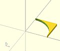difference ( and not )
square - circle
difference ( and not )
circle - square
intersection ( and )
circle - (circle - square)

 union()       {square(10);circle(10);} // square or  circle
 difference()  {square(10);circle(10);} // square and not circle
 difference()  {circle(10);square(10);} // circle and not square
 intersection(){square(10);circle(10);} // square and circle

3D examples

union ( or )
sphere + cube
difference ( and not )
cube - sphere
difference ( and not )
sphere - cube
intersection ( and )
sphere - (sphere - cube)

 union()       {cube(12, center=true); sphere(8);} // cube or  sphere
 difference()  {cube(12, center=true); sphere(8);} // cube and not sphere
 difference()  {sphere(8); cube(12, center=true);} // sphere and not cube
 intersection(){cube(12, center=true); sphere(8);} // cube and sphere

union

Creates a union of all its child nodes. This is the sum of all children (logical or).
May be used with either 2D or 3D objects, but don't mix them.

 //Usage example:
 union() {
 	cylinder (h = 4, r=1, center = true, $fn=100);
 	rotate ([90,0,0]) cylinder (h = 4, r=0.9, center = true, $fn=100);
 }

Remark: union is implicit when not used. But it is mandatory, for example, in difference to group first child nodes into one.

Note: It is mandatory for all unions, explicit or implicit, that external faces to be merged not be coincident. Failure to follow this rule results in a design with undefined behavior, and can result in a render which is not manifold (with zero volume portions, or portions inside out), which typically leads to a warning and sometimes removal of a portion of the design from the rendered output. (This can also result in flickering effects during the preview.) This requirement is not a bug, but an intrinsic property of floating point comparisons and the fundamental inability to exactly represent irrational numbers such as those resulting from most rotations. As an example, this is an invalid OpenSCAD program, and will at least lead to a warning on most platforms:

 // Invalid!
 size = 10;
 rotation = 17;
 union() {
    rotate([rotation, 0, 0])
       cube(size);
    rotate([rotation, 0, 0])
       translate([0, 0, size])
       cube([2, 3, 4]);
 }

The solution is to always use a small value called an epsilon when merging adjacent faces like this to guarantee overlap. Note the 0.01 eps value used in TWO locations, so that the external result is equivalent to what was intended:

 // Correct!
 size = 10;
 rotation = 17;
 eps = 0.01;
 union() {
    rotate([rotation, 0, 0])
       cube(size);
    rotate([rotation, 0, 0])
       translate([0, 0, size-eps])
       cube([2, 3, 4+eps]);
 }

difference

Subtracts the 2nd (and all further) child nodes from the first one (logical and not).
May be used with either 2D or 3D objects, but don't mix them.

Usage example:
difference() {
	cylinder (h = 4, r=1, center = true, $fn=100);
	rotate ([90,0,0]) cylinder (h = 4, r=0.9, center = true, $fn=100);
}

Note: It is mandatory that surfaces that are to be removed by a difference operation have an overlap, and that the negative piece being removed extends fully outside of the volume it is removing that surface from. Failure to follow this rule can cause preview artifacts and can result in non-manifold render warnings or the removal of pieces from the render output. See the description above in union for why this is required and an example of how to do this by this using a small epsilon value.

difference with multiple children

Note, in the second instance, the result of adding a union of the 1st and 2nd children.

// Usage example for difference of multiple children:
$fn=90;
difference(){
                                            cylinder(r=5,h=20,center=true);
    rotate([00,140,-45]) color("LightBlue") cylinder(r=2,h=25,center=true);
    rotate([00,40,-50])                     cylinder(r=2,h=30,center=true);
    translate([0,0,-10])rotate([00,40,-50]) cylinder(r=1.4,h=30,center=true);
}
   
// second instance with added union
translate([10,10,0]){
    difference(){
      union(){        // combine 1st and 2nd children
                                                cylinder(r=5,h=20,center=true);
        rotate([00,140,-45]) color("LightBlue") cylinder(r=2,h=25,center=true);
      }
      rotate([00,40,-50])                       cylinder(r=2,h=30,center=true);
      translate([0,0,-10])rotate([00,40,-50])   cylinder(r=1.4,h=30,center=true);
    }
}

intersection

Creates the intersection of all child nodes. This keeps the overlapping portion (logical and).
Only the area which is common or shared by all children is retained.
May be used with either 2D or 3D objects, but don't mix them.

//Usage example:
intersection() {
	cylinder (h = 4, r=1, center = true, $fn=100);
	rotate ([90,0,0]) cylinder (h = 4, r=0.9, center = true, $fn=100);
}

render

Warning: Using render, always calculates the CSG model for this tree (even in OpenCSG preview mode). This can make previewing very slow and OpenSCAD to appear to hang/freeze.

Usage example:
render(convexity = 1) { ... }

convexity

Integer. The convexity parameter specifies the maximum number of front and back sides a ray intersecting the object might penetrate. This parameter is only needed for correctly displaying the object in OpenCSG preview mode and has no effect on the polyhedron rendering.

This image shows a 2D shape with a convexity of 4, as the ray indicated in red crosses the 2D shape a maximum of 4 times. The convexity of a 3D shape would be determined in a similar way. Setting it to 10 should work fine for most cases.

The text in its current form is incomplete.

Modifier characters are used to change the appearance or behaviors of child nodes. They are particularly useful in debugging where they can be used to highlight specific objects, or include or exclude them from rendering.

Advanced concept

OpenSCAD uses different libraries to implement capabilities, and this can introduce some inconsistencies to the F5 preview behavior of transformations. Traditional transforms (translate, rotate, scale, mirror & multimatrix) are performed using OpenGL in preview, while other more advanced transforms, such as resize, perform a CGAL operation, behaving like a CSG operation affecting the underlying object, not just transforming it. In particular this can affect the display of modifier characters, specifically "#" and "%", where the highlight may not display intuitively, such as highlighting the pre-resized object, but highlighting the post-scaled object.

Note: The color changes triggered by character modifiers appear only in "Compile" mode, not "Compile and Render (CGAL)" mode. (As per the color section.)

Background modifier

Ignore this subtree for the normal rendering process and draw it in transparent gray (all transformations are still applied to the nodes in this tree).

Because the marked subtree is completely ignored, it might have unexpected effects in case it's used, for example, with the first object in a difference(). In that case this object is rendered in transparent gray, but it is not used as the base for the difference()!

Usage

 % { ... }

Example

difference() {
	cylinder (h = 12, r=5, center = true, $fn=100);
	// first object to be subtracted
	rotate ([90,0,0]) cylinder (h = 15, r=1, center = true, $fn=100);
	// second object to be subtracted
	%rotate ([0,90,0]) cylinder (h = 15, r=3, center = true, $fn=100);
}

Example output

Output without the modifier.

Output with modifier added.

Rendered Model.

Debug modifier

Use this subtree as usual in the rendering process but also draw it unmodified in transparent pink.

Usage

 # { ... }

Example

difference() {
	// start objects
	cylinder (h = 12, r=5, center = true, $fn=100);
        // first object to be subtracted
	#rotate ([90,0,0]) cylinder (h = 15, r=1, center = true, $fn=100);
        // second object to be subtracted
	#rotate ([0,90,0]) cylinder (h = 15, r=3, center = true, $fn=100);
}

Example output

Output without the modifier.

Output with modifier added.

Root modifier

Ignore the rest of the design and use this subtree as design root.

Usage

 ! { ... }

Example

difference() {
	cube(10, center = true);
	translate([0, 0, 5]) {
		!rotate([90, 0, 0]) {
			#cylinder(r = 2, h = 20, center = true, $fn = 40);
		}
	}
}

Example output

Output without the modifier.

Output with modifier added.

As shown in the example output with the root modifier active, the rotate() is executed as it's part of the subtree marked with the root modifier, but the translate() has no effect.

Disable modifier

Simply ignore this entire subtree.

Usage

 * { ... }

Example

difference() {
	cube(10, center = true);
	translate([0, 0, 5]) {
		rotate([0, 90, 0]) {
			cylinder(r = 2, h = 20, center = true, $fn = 40);
		}
		*rotate([90, 0, 0]) {
			#cylinder(r = 2, h = 20, center = true, $fn = 40);
		}
	}
}

Example output

Output without the modifier.

Output with modifier added.

The disable modifier allows you to comment out one or multiple subtrees. Compared to using the usual line or multi-line comments, it's aware of the hierarchical structure, which makes it easier to disable even larger trees without the need to search for the end of the subtree.

Echo statements

See also: OpenSCAD User Manual/Other Language Features#Echo function

This function prints the contents to the compilation window (aka Console). Useful for debugging code. Also see the String function str().

Numeric values are rounded to 5 significant digits.

It can be handy to use 'variable=variable' as the expression to easily label the variables, see the example below.

Usage examples:

my_h=50;
my_r=100;
echo("This is a cylinder with h=", my_h, " and r=", my_r);
echo(my_h=my_h,my_r=my_r); // shortcut
cylinder(h=my_h, r=my_r);

Shows in the Console as

ECHO: "This is a cylinder with h=", 50, " and r=", 100
ECHO: my_h = 50, my_r = 100

Users can extend the language by defining their own functions and modules. This allows grouping portions of script for easy reuse with different values. Well chosen names also help document your script.

Functions return values.

Modules perform actions, but do not return values.

OpenSCAD calculates the value of variables at compile-time, not run-time. The last variable assignment within a scope applies everywhere in that scope. It also applies to any inner scopes, or children, thereof. See Scope of variables for more details. It may be helpful to think of them as override-able constants rather than as variables.

For functions and modules OpenSCAD makes copies of pertinent portions of the script for each use. Each copy has its own scope, which contains fixed values for variables and expressions unique to that instance.

The name of functions and modules is case sensitive, therefore test() and TEST() refer to different functions/modules.

Scope

Modules and functions can be defined within a module definition, where they are visible only in the scope of that module.

For example

function parabola(f,x) = ( 1/(4*f) ) * x*x; 
module plotParabola(f,wide,steps=1) {
  function y(x) = parabola(f,x);
  module plot(x,y) {
    translate([x,y])
      circle(1,$fn=12);
  }
  xAxis=[-wide/2:steps:wide/2];
  for (x=xAxis) 
    plot(x, y(x));
}
color("red")  plotParabola(10, 100, 5);
color("blue") plotParabola(4,  60,  2);

The function y() and module plot() cannot be called in the global scope.

Functions

Functions operate on values to calculate and return new values.

function definition

function name ( parameters ) = value ;

name: Your name for this function. A meaningful name is helpful later. Currently valid names can only be composed of simple characters and underscores [a-zA-Z0-9_] and do not allow high-ascii or unicode characters.
parameters: Zero or more arguments. Parameters can be assigned default values, to use in case they are omitted in the call. Parameter names are local and do not conflict with external variables of the same name.
value: an expression that calculates a value. This value can be a vector.

Function use

When used, functions are treated as values, and do not themselves end with a semicolon ;.

// example 1
    
function func0() = 5;
function func1(x=3) = 2*x+1;
function func2() = [1,2,3,4];
function func3(y=7) = (y==7) ? 5 : 2 ;
function func4(p0,p1,p2,p3) = [p0,p1,p2,p3];
    
echo(func0());            // 5
a =   func1();            // 7
b =   func1(5);           // 11
echo(func2());            // [1, 2, 3, 4]
echo(func3(2), func3());  // 2, 5
   
z = func4(func0(), func1(), func2(), func3());
//  [5, 7, [1, 2, 3, 4], 5]
   
translate([0, -4*func0(), 0])
  cube([func0(), 2*func0(), func0()]);
// same as translate([0,-20,0]) cube([5,10,5]);

// example 2  creates for() range to give desired no of steps to cover range
  
function steps(start, no_steps, end) =
  [start : (end-start)/(no_steps-1) : end];
  
echo(steps(10, 3, 5));                // [10 : -2.5 : 5]
for (i = steps(10, 3, 5))  echo(i);   //  10 7.5 5
  
echo(steps(10, 3, 15));               // [10 : 2.5 : 15]
for (i = steps(10, 3, 15)) echo(i);   // 10 12.5 15
  
echo(steps(0, 5, 5));                // [0 : 1.25 : 5]
for (i = steps(0, 5, 5))   echo(i);  // 0 1.25 2.5 3.75 5

Example 3

// example 3     rectangle with top pushed over, keeping same y
  
function rhomboid(x=1, y=1, angle=90)
  = [[0,0],[x,0],
    [x+x*cos(angle)/sin(angle),y],
    [x*cos(angle)/sin(angle),y]];
    
echo (v1); v1 = rhomboid(10,10,35);  // [[0, 0], 
                                     // [10, 0], 
                                     // [24.2815, 10],
                                     // [14.2815, 10]]
polygon(v1);
polygon(rhomboid(10,10,35));         // alternate

//performing the same action with a module
   
module parallelogram(x=1,y=1,angle=90)
    {polygon([[0,0],[x,0],
              [x+x*cos(angle)/sin(angle),y],
              [x*cos(angle)/sin(angle),y]]);};
  
parallelogram(10,10,35);

You can also use the let statement to create variables in a function:

function get_square_triangle_perimeter(p1, p2) =
  let (hypotenuse = sqrt(p1*p1+p2*p2))
    p1 + p2 + hypotenuse;

It can be used to store values in recursive functions. See the wikipedia page for more information on the general concept.

Recursive functions

Recursive function calls are supported. Using the Conditional Operator "... ? ... : ... ", it is possible to ensure the recursion is terminated.

// recursion example: add all integers up to n
function add_up_to(n) = ( n==0 ? 0 : n + add_up_to(n-1) );

There is a built-in recursion limit to prevent an application crash (a few thousands). If the limit is hit, you get an error like: ERROR: Recursion detected calling function ... .

For all tail-recursive functions that calls itself, OpenSCAD is able to eliminate internally the recursion transforming it in an iterative loop. The previous example code is not a tail call as an "add" operation need to be calculated after calling. But the following is entitled to tail-recursion elimination:

// tail-recursion elimination example: add all integers up to n
function add_up_to(n, sum=0) =
    n==0 ?
        sum :
        add_up_to(n-1, sum+n);
 
echo(sum=add_up_to(100000));
// ECHO: sum = 5.00005e+009

Tail-recursion elimination allows much higher recursion limits (up to 1000000).

Function literals

[Note: Requires version 2021.01]

Function literals are expressions that define functions, other names for this are lambdas or closures.

function literal

function (x) x + x

Function literals can be assigned to variables and passed around like any value. Calling the function uses the normal function call syntax with parenthesis.

func = function (x) x * x;
echo(func(5)); // ECHO: 25

It's possible to define functions that return functions. Unbound variables are captured by lexical scope.

a = 1;
selector = function (which)
             which == "add"
             ? function (x) x + x + a
             : function (x) x * x + a;
             
echo(selector("add"));     // ECHO: function(x) ((x + x) + a)
echo(selector("add")(5));  // ECHO: 11

echo(selector("mul"));     // ECHO: function(x) ((x * x) + a)
echo(selector("mul")(5));  // ECHO: 26

Overwriting built-in functions

It is possible to overwrite the built-in functions. Note that definitions are handled first, so the evaluation does indeed return true for both echo() calls as those are evaluated in a later processing step.

Source Code	Console output
echo (sin(1)); function sin(x) = true; echo (sin(1));	Compiling design (CSG Tree generation)... ECHO: true ECHO: true Compiling design (CSG Products generation)...

Modules

Modules can be used to define objects or, using children(), define operators. Once defined, modules are temporarily added to the language.

module definition

module name ( parameters ) { actions }

name: Your name for this module. Try to pick something meaningful. Currently valid names can only be composed of simple characters and underscores [a-zA-Z0-9_] and do not allow high-ascii or unicode characters.
parameters: Zero or more arguments. Parameters may be assigned default values, to use in case they are omitted in the call. Parameter names are local and do not conflict with external variables of the same name.
actions: Nearly any statement valid outside a module can be included within a module. This includes the definition of functions and other modules. Such functions and modules can be called only from within the enclosing module.

Variables can be assigned, but their scope is limited to within each individual use of the module. There is no mechanism in OpenSCAD for modules to return values to the outside. See Scope of variables for more details.

Object modules

Object modules use one or more primitives, with associated operators, to define new objects.

In use, object modules are actions ending with a semi-colon ';'.

name ( parameter values );

Color bar

//example 1
   
translate([-30,-20,0])
   ShowColorBars(Expense);
   
ColorBreak=[[0,""],
           [20,"lime"],  // upper limit of color range
           [40,"greenyellow"],
           [60,"yellow"],
           [75,"LightCoral"],
           [200,"red"]];
Expense=[16,20,25,85,52,63,45];
   
module ColorBar(value,period,range){  // 1 color on 1 bar
   RangeHi = ColorBreak[range][0];
   RangeLo = ColorBreak[range-1][0];
   color( ColorBreak[range][1] ) 
   translate([10*period,0,RangeLo])
      if (value > RangeHi)      cube([5,2,RangeHi-RangeLo]);
      else if (value > RangeLo) cube([5,2,value-RangeLo]);
  }  
module ShowColorBars(values){
    for (month = [0:len(values)-1], range = [1:len(ColorBreak)-1])
      ColorBar(values[month],month,range);
}

House

//example 2
module house(roof="flat",paint=[1,0,0]) {
   color(paint)
   if(roof=="flat") { translate([0,-1,0]) cube(); }
   else if(roof=="pitched") {
     rotate([90,0,0]) linear_extrude(height=1)
     polygon(points=[[0,0],[0,1],[0.5,1.5],[1,1],[1,0]]); }
   else if(roof=="domical") {
     translate([0,-1,0]){
       translate([0.5,0.5,1]) sphere(r=0.5,$fn=20); cube(); }
} }

                   house();
translate([2,0,0]) house("pitched");
translate([4,0,0]) house("domical",[0,1,0]);
translate([6,0,0]) house(roof="pitched",paint=[0,0,1]);
translate([0,3,0]) house(paint=[0,0,0],roof="pitched");
translate([2,3,0]) house(roof="domical");
translate([4,3,0]) house(paint=[0,0.5,0.5]);

//example 3
   
element_data = [[0,"","",0],  // must be in order
    [1,"Hydrogen","H",1.008],   // indexed via atomic number
    [2,"Helium",  "He",4.003]   // redundant atomic number to preserve your sanity later
];
   
Hydrogen = 1;
Helium   = 2;
      
module coaster(atomic_number){
    element     = element_data[atomic_number][1];
    symbol      = element_data[atomic_number][2];
    atomic_mass = element_data[atomic_number][3];
    //rest of script
}

Operator modules

Children

Use of children() allows modules to act as operators applied to any or all of the objects within this module instantiation. In use, operator modules do not end with a semi-colon.

name ( parameter values ){scope of operator}

Basicly the children() command is used to apply modifications to objects that are focused by a scope:

 module myModification() { rotate([0,45,0]) children(); } 
 
 myModification()                 // The modification
 {                                // Begin focus
   cylinder(10,4,4);              // First child
   cube([20,2,2], true);          // Second child
 }                                // End focus

Objects are indexed via integers from 0 to $children-1. OpenSCAD sets $children to the total number of objects within the scope. Objects grouped into a sub scope are treated as one child. See example of separate children below and Scope of variables. Note that children(), echo() and empty block statements (including ifs) count as $children objects, even if no geometry is present (as of v2017.12.23).

 children();                         all children
 children(index);                    value or variable to select one child
 children([start : step : end]);     select from start to end incremented by step
 children([start : end]);            step defaults to 1 or -1
 children([vector]);                 selection of several children

Deprecated child() module

Up to release 2013.06 the now deprecated child() module was used instead. This can be translated to the new children() according to the table:

up to 2013.06	2014.03 and later
child()	children(0)
child(x)	children(x)
for (a = [0:$children-1]) child(a)	children([0:$children-1])

Use all children

Examples

//Use all children
    
module move(x=0,y=0,z=0,rx=0,ry=0,rz=0)
{ translate([x,y,z])rotate([rx,ry,rz]) children(); }
   
move(10)           cube(10,true);
move(-10)          cube(10,true);
move(z=7.07, ry=45)cube(10,true);
move(z=-7.07,ry=45)cube(10,true);

Use only the first child, multiple times

//Use only the first child, multiple times
  
module lineup(num, space) {
   for (i = [0 : num-1])
     translate([ space*i, 0, 0 ]) children(0);
}

lineup(5, 65){ sphere(30);cube(35);}

Separate action for each child

  //Separate action for each child
   
  module SeparateChildren(space){
    for ( i= [0:1:$children-1])   // step needed in case $children < 2  
      translate([i*space,0,0]) {children(i);text(str(i));}
  }
   
  SeparateChildren(-20){
    cube(5);              // 0
    sphere(5);            // 1
    translate([0,20,0]){  // 2
      cube(5);
      sphere(5);
    }     
    cylinder(15);         // 3
    cube(8,true);         // 4
  }
  translate([0,40,0])color("lightblue")
    SeparateChildren(20){cube(3,true);}

Multiple ranges

//Multiple ranges
module MultiRange(){
   color("lightblue") children([0:1]);
   color("lightgreen")children([2:$children-2]);
   color("lightpink") children($children-1);
}
   
MultiRange()
{
   cube(5);              // 0
   sphere(5);            // 1
   translate([0,20,0]){  // 2
     cube(5);
     sphere(5);
   }     
   cylinder(15);         // 3
   cube(8,true);         // 4
}

Further module examples

Objects

module arrow(){
    cylinder(10);
    cube([4,.5,3],true);
    cube([.5,4,3],true);
    translate([0,0,10]) cylinder(4,2,0,true);
}
  
module cannon(){
    difference(){union()
      {sphere(10);cylinder(40,10,8);} cylinder(41,4,4);
} }
  
module base(){
    difference(){
      cube([40,30,20],true);
      translate([0,0,5])  cube([50,20,15],true);
} }

Operators

Rotary Clusters

module aim(elevation,azimuth=0)
    { rotate([0,0,azimuth])
      { rotate([0,90-elevation,0]) children(0);
      children([1:1:$children-1]);   // step needed in case $children < 2
} }
   
aim(30,20)arrow();
aim(35,270)cannon();
aim(15){cannon();base();}

module RotaryCluster(radius=30,number=8)
    for (azimuth =[0:360/number:359])
      rotate([0,0,azimuth])    
        translate([radius,0,0]) { children();
          translate([40,0,30]) text(str(azimuth)); }
   
RotaryCluster(200,7) color("lightgreen") aim(15){cannon();base();}
rotate([0,0,110]) RotaryCluster(100,4.5) aim(35)cannon();
color("LightBlue")aim(55,30){cannon();base();}

Recursive modules

Like functions, modules may contain recursive calls. However, there is no tail-recursion elimination for recursive modules.

The code below generates a crude model of a tree. Each tree branch is itself a modified version of the tree and produced by recursion. Be careful to keep the recursion depth (branching) n below 7 as the number of primitives and the preview time grow exponentially.

A simple tree created with a recursive OpenSCAD module

    module simple_tree(size, dna, n) {   
        if (n > 0) {
            // trunk
            cylinder(r1=size/10, r2=size/12, h=size, $fn=24);
            // branches
            translate([0,0,size])
                for(bd = dna) {
                    angx = bd[0];
                    angz = bd[1];
                    scal = bd[2];
                        rotate([angx,0,angz])
                            simple_tree(scal*size, dna, n-1);
                }
        }
        else { // leaves
            color("green")
            scale([1,1,3])
                translate([0,0,size/6]) 
                    rotate([90,0,0]) 
                        cylinder(r=size/6,h=size/10);
        }
    }
    // dna is a list of branching data bd of the tree:
    //      bd[0] - inclination of the branch
    //      bd[1] - Z rotation angle of the branch
    //      bd[2] - relative scale of the branch
    dna = [ [12,  80, 0.85], [55,    0, 0.6], 
            [62, 125, 0.6], [57, -125, 0.6] ];
    simple_tree(50, dna, 5);

Another example of recursive module may be found in Tips and Tricks

Overwriting built-in modules

It is possible to overwrite the built-in modules.

A simple, but pointless example would be:

module sphere(){
    square();
}
sphere();

Note that the built-in sphere module can not be called when over written.

A more sensible way to use this language feature is to overwrite the 3D primitives with extruded 2D-primitives. This allows additional to customize the default parameters and to add additional parameters. For including code from external files in OpenSCAD, there are two commands available:

include <filename> acts as if the contents of the included file were written in the including file, and
use <filename> imports modules and functions, but does not execute any commands other than those definitions.

Library files are searched for in the same folder as the design was opened from, in the library folder of the OpenSCAD installation, and in folders given by the OPENSCADPATH environment variable. You can use a relative path specification to either. If they lie elsewhere you must give the complete path. Newer versions have predefined user libraries, see the OpenSCAD_User_Manual/Libraries page, which also documents a number of library files included in OpenSCAD.

Wildcards (*, for e.g. include <MCAD/*.scad>) can not be used to include multiple files.

Directory separators

Windows and Linux/Mac use different separators for directories. Windows uses \, e.g. directory\file.ext, while the others use /, e.g. directory/file.ext. This could lead to cross platform issues. However OpenSCAD on Windows correctly handles the use of /, so using / in all include or use statements work on all platforms.

To access the parent directory ../ can be used under Linux.

Variables

Scope of variables

Using include <filename> allows default variables to be specified in the library. These defaults can be overridden in the main code. An OpenSCAD variable has only one value during the life of the program. When there are multiple assignments it takes the last value, but assigns when the variable is first created. This has an effect when assigning in a library, as any variables that you later use to change the default, must be assigned before the include statement. See the second example below.

Overwriting variables

Default variables in an include can be overridden, for example

lib.scad

i=1;
k=3;
module x() {
    echo("hello world");
    echo("i=",i,"j=",j,"k=",k);
}

hello.scad

j=4;
include <lib.scad>
x();
i=5;
x();
k=j;
x();

Produces the following

ECHO: "hello world"
ECHO: "i=", 5, "j=", 4, "k=", 4
ECHO: "hello world"
ECHO: "i=", 5, "j=", 4, "k=", 4
ECHO: "hello world"
ECHO: "i=", 5, "j=", 4, "k=", 4

However, placing j=4; after the include fails, producing

ECHO: "hello world"
ECHO: "i=", 5, "j=", 4, "k=", undef
ECHO: "hello world"
ECHO: "i=", 5, "j=", 4, "k=", undef
ECHO: "hello world"
ECHO: "i=", 5, "j=", 4, "k=", undef

Example "Ring-Library"

A library file for generating rings might look like this (defining a function and providing an example):

ring.scad:

module ring(r1, r2, h) {
    difference() {
        cylinder(r = r1, h = h);
        translate([ 0, 0, -1 ]) cylinder(r = r2, h = h+2);
    }
}

ring(5, 4, 10);

Including the library using

include <ring.scad>
rotate([90, 0, 0]) ring(10, 1, 1);

would result in the example ring being shown in addition to the rotated ring, but

use <ring.scad>
rotate([90, 0, 0]) ring(10, 1, 1);

shows only the rotated ring.

If using the use function, make sure to place the use statements at top of the file, or at least not within a module!

This works fine:

 // a.scad
 use <ring.scad>
 module a() {
   ring();
 }

but this results in an syntax error:

 //a.scad
 module a() {
   use <ring.scad>
   ring();
 }

Nested Include and Use

OpenSCAD executes nested calls to include and use. There is one caveat to this, that use brings functions and modules only into the local file context. As a result, nested calls to use have no effect on the environment of the base file; the child use call works in the parent use context, but the modules and functions so imported fall out of context before they are seen by the base context.

The text in its current form is incomplete.

Special variables

Special variables provide an alternate means of passing arguments to modules and functions. All user, or OpenSCAD, defined variables starting with a '$' are special variables, similar to special variables in lisp. Modules and function see all outside variables in addition to those passed as arguments or defined internally.

Currently valid special variable names can only be composed of $ followed by simple characters and underscores [a-zA-Z0-9_] and do not allow high-ascii or unicode characters.

The value for a regular variable is assigned at compile time and is thus static for all calls.

Special variables pass along their value from within the scope (see scope of variables) from which the module or function is called. This means that special variables can potentially have a different value each time a module or function is called.

regular  = "regular global";
$special = "special global";
module show() echo("         in show    ", regular,"   ", $special );

echo ("         outside    ", regular,"   ", $special );
          // ECHO: "         outside    ", "regular global", "   ", "special global"
  
for ( regular = [0:1] ){ echo("in regular loop     ", regular,"   ", $special ); show();}
          // ECHO: "in regular loop     ", 0, "   ", "special global"
          // ECHO: "         in show    ", "regular global", "   ", "special global"
          // ECHO: "in regular loop     ", 1, "   ", "special global"
          // ECHO: "         in show    ", "regular global", "   ", "special global"

for ( $special = [5:6] ){ echo("in special loop     ", regular,"   ", $special ); show();}
          // ECHO: "in special loop     ", "regular global", "   ", 5
          // ECHO: "         in show    ", "regular global", "   ", 5
          // ECHO: "in special loop     ", "regular global", "   ", 6
          // ECHO: "         in show    ", "regular global", "   ", 6

show();
          // ECHO: "         in show    ", "regular global", "   ", "special global"

This is useful when multiple arguments need to be passed thru several layers of module calls.

Several special variables are already defined by OpenSCAD.

Circle resolution: $fa, $fs, and $fn

The $fa, $fs, and $fn special variables control the number of facets used to generate an arc:

$fa is the minimum angle for a fragment. Even a huge circle does not have more fragments than 360 divided by this number. The default value is 12 (i.e. 30 fragments for a full circle). The minimum allowed value is 0.01. Attempting to set a lower value causes a warning.

$fs is the minimum size of a fragment. The default value is 2 so very small circles have a smaller number of fragments than specified using $fa. The minimum allowed value is 0.01. Attempting to set a lower value causes a warning.

$fn is number of fragments and usually has the default value of 0. When this variable has a value greater than zero, the other two variables are ignored, and a full circle is rendered using this number of fragments.

The higher the number of fragments, the more memory and CPU consumed; large values can bring many systems to their knees. Depending on the design, $fn values, and the corresponding results of $fa & $fs, should be kept small, at least until the design is finalised when it can be increased for the final result. A $fn over 128 is not recommended or only for specific circumstances, and below 50 would be advisable for performance.

You can also use two different values for preview and render

     $fn = $preview ? 32 : 64;

TIP: If you want to create a circle/cylinder/sphere which has an axis aligned integer bounding box (i.e. a bounding box that has integral dimensions, and an integral position) use a value of $fn that is divisible by 4.

When $fa and $fs are used to determine the number of fragments for a circle, then OpenSCAD never uses fewer than 5 fragments.

This is the C code that calculates the number of fragments in a circle:

      int get_fragments_from_r(double r, double fn, double fs, double fa)
      {
             if (r < GRID_FINE) return 3;
             if (fn > 0.0) return (int)(fn >= 3 ? fn : 3);
             return (int)ceil(fmax(fmin(360.0 / fa, r*2*M_PI / fs), 5));
      }

Or you can embed this OpenSCAD version in your code to work out what's going on, you need to set r= to your size

   echo(n=($fn>0?($fn>=3?$fn:3):ceil(max(min(360/$fa,r*2*PI/$fs),5))),a_based=360/$fa,s_based=r*2*PI/$fs);

Spheres are first sliced into as many slices as the number of fragments being used to render a circle of the sphere's radius, and then every slice is rendered into as many fragments as are needed for the slice radius. You might have recognized already that the pole of a sphere is usually a pentagon. This is why.

The number of fragments for a cylinder is determined using the greater of the two radii.

The method is also used when rendering circles and arcs from DXF files. The variables have no effect when importing STL files.

You can generate high resolution spheres by resetting the $fX values in the instantiating module:

      $fs = 0.01;
      sphere(2);

or simply by passing the special variable as parameter:

      sphere(2, $fs = 0.01);

You can even scale the special variable instead of resetting it:

      sphere(2, $fs = $fs * 0.01);

Animation: $t

Simple harmonic motion, 20 FPS, 100 steps

Animated gears 17T and 31T

The $t variable is used in "rotate" and "translate" for animation, $t*360 giving complete cycles. To start animation, select View\Animate and enter values for "FPS" and "Steps". The "Time" field shows the current value of $t as a decimal fraction.

Simple harmonic motion

translate ([0, 0, 10*sin($t*360)])

sphere(2);

gives a sphere that oscillates between -10 and +10 on the Z-axis.

Rotation

rotate ([0, 0, $t*360])

square(5);

rotates a square around one corner around the Z-axis. To rotate the square about its middle, use:

rotate ([0, 0, $t*360])

square(5, center=true);

Part-rotation

All parts in an animation complete one cycle of motion in the same time, $t, jump back to zero, and start again. However, the cycles can be given different numbers of steps, to give the illusion of different speeds in the same animation. This can be used to animate meshing gears of different sizes.

rotate([0, 0, $t*360/17])

gear(teeth=17);

and

rotate([0, 0, -$t*360/31])

gear(teeth=31);

Circular orbit

rotate ([0, 0, $t*360])

translate ([10, 0])

square(5, center=true);

Circular orbit without rotation

rotate ([0, 0, $t*360])

translate ([9, 0])

Elliptical orbit

rotate ([0, 0, -$t*360])

square(5, center=true);

Elliptical orbit

translate([10*sin($t*360), 20*cos($t*360)])

square(2, center=true);

Note that with "translate", the object does not rotate.

Elliptical motion

e=10;

rotate([0, 0, $t*360])

translate([e, 0])

rotate([0, 0, -$t*720])

square([2*e, 2], center=true);

If "Dump Pictures" is checked, then images are created in the same directory as the .scad file. The exported PNG files can be turned into a gif via command line:

convert -delay 10 -loop 0 *.png myimage.gif

where -delay 10 is the duration of each frame in milliseconds, and -loop 0 specifies the number of loops (0 = loop forever).

The Linux convert command is part of ImageMagick, which can also be installed on macOS and Windows. Additional parameters are possible for cropping and scaling.

Viewport: $vpr, $vpt, $vpf and $vpd

These contain the current viewport rotation and translation and camera distance - at the time of doing the rendering. Moving the viewport does not update them. During an animation they are updated for each frame.

$vpr shows rotation
$vpt shows translation (i.e. won't be affected by rotate and zoom)
$vpf shows the FOV (Field of View) of the view [Note: Requires version 2021.01]
$vpd shows the camera distance [Note: Requires version 2015.03]

Example

 cube([10, 10, $vpr[0] / 10]);

which makes the cube change size based on the view angle, if an animation loop is active (which does not need to use the $t variable)

You can also make bits of a complex model vanish as you change the view.

All four variables are writable, but only assignments at the top-level of the main file has an effect on the viewport. [Note: Requires version 2015.03]

Example

 $vpr = [0, 0, $t * 360];

which allows a simple 360 degree rotation around the Z axis in animation mode.

The menu command Edit - Paste Viewport Rotation/Translation copies the current value of the viewport, but not the current $vpr or $vpt.

Execution mode: $preview

[Note: Requires version 2019.05]

$preview is true, when in OpenCSG preview (F5). $preview is false, when in render (F6).

This can, for example, be used to reduce detail during preview to save time, without losing detail in the final rendered result:

$fn = $preview ? 12 : 72;
sphere(r = 1);

Note that the render module does not affect $preview:

render(){
    $fn = $preview ? 12 : 72;
    sphere(r = 1);
}

Another use could be to make the preview show an assembly view and the render generate just the printed parts laid out for printing.

If printed parts need extra features that are removed post printing, for example support for suspended holes, then the preview can omit these to show the finished part after post processing.

When OpenSCAD is run from the command line $preview is only true when generating a PNG image with OpenCSG. It is false when generating STL, DXF and SVG files with CGAL. It is also false when generating CSG and ECHO files. This may or may not be what you want, but you can always override it on the command line like any other variable with the -D option.

Echo module

The echo() module prints the contents to the compilation window (aka Console). Useful for debugging code. Also see the String function str().

Numeric values are rounded to 5 significant digits.

It can be handy to use 'variable=variable' as the expression to easily label the variables, see the example below.

Usage examples:

my_h=50;
my_r=100;
echo("This is a cylinder with h=", my_h, " and r=", my_r);
echo(my_h=my_h,my_r=my_r); // shortcut
cylinder(h=my_h, r=my_r);

Shows in the Console as

ECHO: "This is a cylinder with h=", 50, " and r=", 100
ECHO: my_h = 50, my_r = 100

Note that the output will not have the extra double quotes and commas if converted to a string using str().

Rounding examples

An example for the rounding:

a=1.0;
b=1.000002;
echo(a);
echo(b);

if(a==b){ //while echoed the same, the values are still distinct 
    echo ("a==b");
}else if(a>b){
    echo ("a>b");
}else if(a<b){
    echo ("a<b");
}else{
    echo ("???");
}

Small and large Numbers

c=1000002;
d=0.000002;
echo(c); //1e+06
echo(d); //2e-06

HTML

HTML output is not officially supported, however depending on the OpenSCAD version, some HTML tags were rendered in the console window.

Echo function

[Note: Requires version 2019.05]

Echo can be used in expression context to print information while the function/expression is evaluated. The output is generated before the expression evaluation to allow debugging of recursive functions.

Example

 a = 3; b = 5;
 
 // echo() prints values before evaluating the expression
 r1 = echo(a, b) a * b; // ECHO: 3, 5
 
 // using let it's still easy to output the result
 r2 = let(r = 2 * a * b) echo(r) r; // ECHO: 30
 
 // use echo statement for showing results 
 echo(r1, r2); // ECHO: 15, 30

A more complex example shows how echo() can be used in both descending and ascending path of a recursive function. The result() helper function is a simple way to output the value of an expression after evaluation.

Example printing both input values and result of recursive sum()

 v = [4, 7, 9, 12];
 function result(x) = echo(result = x) x;
 function sum(x, i = 0) = echo(str("x[", i, "]=", x[i])) result(len(x) > i ? x[i] + sum(x, i + 1) : 0);
 echo("sum(v) = ", sum(v));
 
 // ECHO: "x[0]=4"
 // ECHO: "x[1]=7"
 // ECHO: "x[2]=9"
 // ECHO: "x[3]=12"
 // ECHO: "x[4]=undef"
 // ECHO: result = 0
 // ECHO: result = 12
 // ECHO: result = 21
 // ECHO: result = 28
 // ECHO: result = 32
 // ECHO: "sum(v) = ", 32

render

example in preview

render() effects show edges

Forces the generation of a mesh even in preview mode. This is useful in certain situations, e.g. when the boolean operations become too slow to track.

Render can also be used (typically in conjunction with convexity) to avoid/workaround preview artifacts.^[1] See also OpenSCAD User Manual/FAQ#Why are some parts (e.g. holes) of the model not rendered correctly?

Usage examples: (Needs description)

render(convexity = 2) difference() {
 cube([20, 20, 150], center = true);
 translate([-10, -10, 0])
  cylinder(h = 80, r = 10, center = true);
 translate([-10, -10, +40])
  sphere(r = 10);
 translate([-10, -10, -40])
  sphere(r = 10);
}

surface

Surface reads Heightmap information from text or image files.

Parameters

file: String. The path to the file containing the heightmap data.

center: Boolean. This determines the positioning of the generated object. If true, object is centered in X- and Y-axis. Otherwise, the object is placed in the positive quadrant. Defaults to false.

invert: Boolean. Inverts how the color values of imported images are translated into height values. This has no effect when importing text data files. Defaults to false. [Note: Requires version 2015.03]

convexity: Integer. The convexity parameter specifies the maximum number of front sides (back sides) a ray intersecting the object might penetrate. This parameter is only needed for correctly displaying the object in OpenCSG preview mode and has no effect on the final rendering.

Text file format

The format for text based height maps is a matrix of numbers which represent the heights for specific points. Rows are mapped in Y-axis direction, columns in X axis direction, with one unit increment between adjacent rows and columns. The numbers must be separated by spaces or tabs. Empty lines and lines starting with a # character are ignored.

Images

[Note: Requires version 2015.03]

Currently only PNG images are supported. Alpha channel information of the image is ignored and the height for the pixel is determined by converting the color value to Grayscale using the linear luminance for the sRGB color space (Y = 0.2126R + 0.7152G + 0.0722B). The gray scale values are scaled to be in the range 0 to 100.

Examples

Example 1:

//surface.scad
surface(file = "surface.dat", center = true, convexity = 5);
%translate([0,0,5])cube([10,10,10], center =true);

#surface.dat
10 9 8 7 6 5 5 5 5 5 
9 8 7 6 6 4 3 2 1 0 
8 7 6 6 4 3 2 1 0 0
7 6 6 4 3 2 1 0 0 0
6 6 4 3 2 1 1 0 0 0
6 6 3 2 1 1 1 0 0 0
6 6 2 1 1 1 1 0 0 0
6 6 1 0 0 0 0 0 0 0
3 1 0 0 0 0 0 0 0 0
3 0 0 0 0 0 0 0 0 0

Result:

Example 2

// example010.dat generated using octave or matlab:
d = (sin(1:0.2:10)' * cos(1:0.2:10)) * 10;
save("-ascii", "example010.dat", "d");

//original surface
surface(file = "example010.dat", center = true, convexity = 5);
//rotated surface
translate(v = [70, 0, 0]) rotate(45, [0, 0, 1]) surface(file = "example010.dat", center = true, convexity = 5);

//intersection
translate(v = [35, 60, 0])
intersection() {
    surface(file = "example010.dat", center = true, convexity = 5);
    rotate(45, [0, 0, 1]) surface(file = "example010.dat", center = true, convexity = 5);
}

Example 3:

[Note: Requires version 2015.03]

// Example 3a
scale([1, 1, 0.1])
  surface(file = "smiley.png", center = true);

// Example 3b
scale([1, 1, 0.1])
  surface(file = "smiley.png", center = true, invert = true);

Input image

Example 3a: surface(invert = false)

Example 3b: surface (invert = true)

Example 3: Using surface() with a PNG image as heightmap input.

Example 4:

[Note: Requires version 2015.03]

// Example 4
surface(file = "BRGY-Grey.png", center = true, invert = false);

PNG Test File
3D Surface

search

The search() function is a general-purpose function to find one or more (or all) occurrences of a value or list of values in a vector, string or more complex list-of-list construct.

Search usage

search( match_value , string_or_vector [, num_returns_per_match [, index_col_num ] ] );

Search arguments

match_value

Can be a single string value. Search loops over the characters in the string and searches for each one in the second argument. The second argument must be a string or a list of lists (this second case is not recommended). The search function does not search for substrings.
Can be a single numerical value.
Can be a list of values. The search function searches for each item on the list.
To search for a list or a full string give the list or string as a single element list such as ["abc"] to search for the string "abc" (See Example 9) or [[6,7,8]] to search for the list [6,7,8]. Without the extra brackets, search looks separately for each item in the list.
If match_value is boolean then search returns undef.

string_or_vector

The string or vector to search for matches.
If match_value is a string then this should be a string and the string is searched for individual character matches to the characters in match_value
If this is a list of lists, v=[[a0,a1,a2...],[b0,b1,b2,...],[c0,c1,c2,...],...] then search looks only at one index position of the sublists. By default this is position 0, so the search looks only at a0, b0, c0, etc. The index_col_num parameter changes which index is searched.
If match_value is a string and this parameter is a list of lists then the characters of the string are tested against the appropriate index entry in the list of lists. However, if any characters fail to find a match a warning message is printed and that return value is excluded from the output (if num_returns_per_match is 1). This means that the length of the output is unpredictable.

num_returns_per_match (default: 1)

By default, search only looks for one match per element of match_value to return as a list of indices
If num_returns_per_match > 1, search returns a list of lists of up to num_returns_per_match index values for each element of match_value.

See Example 8 below.

If num_returns_per_match = 0, search returns a list of lists of all matching index values for each element of match_value.

See Example 6 below.

index_col_num (default: 0)

As noted above, when searching a list of lists, search looks only at one index position of each sublist. That index position is specified by index_col_num.
See Example 5 below for a simple usage example.

Search usage examples

See example023.scad included with OpenSCAD for a renderable example.

Index values return as list

Example	Code	Result
1	`search("a","abcdabcd");`	[0]
2	`search("e","abcdabcd");`	[]
3	`search("a","abcdabcd",0);`	[[0,4]]
4	`data=[ ["a",1],["b",2],["c",3],["d",4],["a",5],["b",6],["c",7],["d",8],["e",9] ];` `search("a", data, num_returns_per_match=0);`	[[0,4]] (see also Example 6 below)

Search on different column; return Index values

Example 5:

 data= [ ["a",1],["b",2],["c",3],["d",4],["a",5],["b",6],["c",7],["d",8],["e",3] ];
 echo(search(3, data));    // Searches index 0, so it doesn't find anything
 echo(search(3, data, num_returns_per_match=0, index_col_num=1));

Outputs:

 ECHO: []
 ECHO: [2, 8]

Search on list of values

Example 6: Return all matches per search vector element.

 data= [ ["a",1],["b",2],["c",3],["d",4],["a",5],["b",6],["c",7],["d",8],["e",9] ];
 search("abc", data, num_returns_per_match=0);

Returns:

   [[0,4],[1,5],[2,6]]

Example 7: Return first match per search vector element; special case return vector.

 data= [ ["a",1],["b",2],["c",3],["d",4],["a",5],["b",6],["c",7],["d",8],["e",9] ];
 search("abc", data, num_returns_per_match=1);

Returns:

   [0,1,2]

Example 8: Return first two matches per search vector element; vector of vectors.

 data= [ ["a",1],["b",2],["c",3],["d",4],["a",5],["b",6],["c",7],["d",8],["e",9] ];
 search("abce", data, num_returns_per_match=2);

Returns:

 [[0,4],[1,5],[2,6],[8]]

Search on list of strings

Example 9:

 lTable2=[ ["cat",1],["b",2],["c",3],["dog",4],["a",5],["b",6],["c",7],["d",8],["e",9],["apple",10],["a",11] ];
 lSearch2=["b","zzz","a","c","apple","dog"];
 l2=search(lSearch2,lTable2);
 echo(str("Default list string search (",lSearch2,"): ",l2));

Returns

 ECHO: "Default list string search (["b", "zzz", "a", "c", "apple", "dog"]): [1, [], 4, 2, 9, 3]"

Getting the right results

// workout which vectors get the results
v=[ ["O",2],["p",3],["e",9],["n",4],["S",5],["C",6],["A",7],["D",8] ];
//
echo(v[0]);					// -> ["O",2]
echo(v[1]);                                     // -> ["p",3]
echo(v[1][0],v[1][1]);                          // -> "p",3
echo(search("p",v));                            // find "p" -> [1]
echo(search("p",v)[0]);                         // -> 1
echo(search(9,v,0,1));                          // find  9  -> [2] 
echo(v[search(9,v,0,1)[0]]);                    // -> ["e",9]
echo(v[search(9,v,0,1)[0]][0]);                 // -> "e"
echo(v[search(9,v,0,1)[0]][1]);                 // -> 9
echo(v[search("p",v,1,0)[0]][1]);               // -> 3
echo(v[search("p",v,1,0)[0]][0]);               // -> "p"
echo(v[search("d",v,1,0)[0]][0]);               // "d" not found -> undef
echo(v[search("D",v,1,0)[0]][1]);               // -> 8

OpenSCAD version

version() and version_num() returns the OpenSCAD version number.

The version() function returns the OpenSCAD version as a vector of three numbers, e.g. [2011, 9, 23]
The version_num() function returns the OpenSCAD version as a number, e.g. 20110923

parent_module(n) and $parent_modules

$parent_modules contains the number of modules in the instantiation stack. parent_module(i) returns the name of the module i levels above the current module in the instantiation stack. The stack is independent of where the modules are defined. It's where they're instantiated that counts. This can, for example, be used to build a BOM (Bill Of Material).

Example:

 module top() {
   children();
 }
 module middle() {
   children();
 }
 top() middle() echo(parent_module(0)); // prints "middle"
 top() middle() echo(parent_module(1)); // prints "top"

assert

[Note: Requires version 2019.05]

Assert evaluates a logical expression. If the expression evaluates to false, the generation of the preview/render is stopped, and an error condition is reported via the console. The report consists of a string representation of the expression and an additional string (optional) that is specified in the assert command.

 assert(condition);
 assert(condition, message);

Parameters

condition: Expression. The expression to be evaluated as check for the assertion.

message: String. Optional message to be output in case the assertion failed.

Example

The simplest example is a simple assert(false);, e.g. in a file named assert_example1.scad.

cube();
assert(false);
sphere();
  
// ERROR: Assertion 'false' failed in file assert_example1.scad, line 2

This example has little use, but the simple assert(false); can be used in code sections that should be unreachable.

Checking parameters

A useful example is checking the validity of input parameters:

module row(cnt = 3){
    // Count has to be a positive integer greater 0
    assert(cnt > 0);
    for (i = [1 : cnt]) {
        translate([i * 2, 0, 0]) sphere();
    }
}

row(0);

// ERROR: Assertion '(cnt > 0)' failed in file assert_example2.scad, line 3

Adding message

When writing a library, it could be useful to output additional information to the user in case of an failed assertion.

module row(cnt = 3){
    assert(cnt > 0, "Count has to be a positive integer greater 0");
    for(i = [1 : cnt]) {
        translate([i * 2, 0, 0]) sphere();
    }
}

row(0);

// ERROR: Assertion '(cnt > 0)': "Count has to be a positive integer greater 0" failed in file assert_example3.scad, line 2

Using assertions in function

Assert returns its children, so when using it in a function you can write

function f(a, b) =
    assert(a < 0, "wrong a") // assert input
    assert(b > 0, "wrong b") // assert input
    let (c = a + b) // derive a new value from input
    assert(c != 0, "wrong c") // assert derived value
    a * b; // calculate

Using the 2D Subsystem

All 2D primitives can be transformed with 3D transformations. They are usually used as part of a 3D extrusion. Although they are infinitely thin, they are rendered with a 1 thickness.

Note: The try to substract with difference() from 3D object will lead to unexpected results in final rendering.

square

Creates a square or rectangle in the first quadrant. When center is true the square is centered on the origin. Argument names are optional if given in the order shown here.

square(size = [x, y], center = true/false);
square(size =  x    , center = true/false);

parameters:

size

single value, square with both sides this length

2 value array [x,y], rectangle with dimensions x and y

center

false (default), 1st (positive) quadrant, one corner at (0,0)

true, square is centered at (0,0)

default values:  square();   yields:  square(size = [1, 1], center = false);

examples:

equivalent scripts for this example
 square(size = 10);
 square(10);
 square([10,10]);
 .
 square(10,false);
 square([10,10],false);
 square([10,10],center=false);
 square(size = [10, 10], center = false);
 square(center = false,size = [10, 10] );

equivalent scripts for this example
 square([20,10],true);
 a=[20,10];square(a,true);

circle

Creates a circle at the origin. All parameters, except r, must be named.

circle(r=radius | d=diameter);

Parameters

r : circle radius. r name is the only one optional with circle.

circle resolution is based on size, using $fa or $fs.

For a small, high resolution circle you can make a large circle, then scale it down, or you could set $fn or other special variables. Note: These examples exceed the resolution of a 3d printer as well as of the display screen.

scale([1/100, 1/100, 1/100]) circle(200); // create a high resolution circle with a radius of 2.
circle(2, $fn=50);                        // Another way.

d : circle diameter (only available in versions later than 2014.03).

$fa : minimum angle (in degrees) of each fragment.

$fs : minimum circumferential length of each fragment.

$fn : fixed number of fragments in 360 degrees. Values of 3 or more override $fa and $fs.

If they are used, $fa, $fs and $fn must be named parameters. click here for more details,.

defaults:  circle(); yields:  circle($fn = 0, $fa = 12, $fs = 2, r = 1);

Equivalent scripts for this example

 circle(10);
 circle(r=10);
 circle(d=20);
 circle(d=2+9*2);

Ellipses

An ellipse can be created from a circle by using either scale() or resize() to make the x and y dimensions unequal. See OpenSCAD User Manual/Transformations

equivalent scripts for this example
 resize([30,10])circle(d=20);
 scale([1.5,.5])circle(d=20);

Regular Polygons

A regular polygon of 3 or more sides can be created by using circle() with $fn set to the number of sides. The following two pieces of code are equivalent.

 circle(r=1, $fn=4);

 module regular_polygon(order = 4, r=1){
     angles=[ for (i = [0:order-1]) i*(360/order) ];
     coords=[ for (th=angles) [r*cos(th), r*sin(th)] ];
     polygon(coords);
 }
 regular_polygon();

These result in the following shapes, where the polygon is inscribed within the circle with all sides (and angles) equal. One corner points to the positive x direction. For irregular shapes see the polygon primitive below.

script for these examples
 translate([-42,  0]){circle(20,$fn=3);%circle(20,$fn=90);}
 translate([  0,  0]) circle(20,$fn=4);
 translate([ 42,  0]) circle(20,$fn=5);
 translate([-42,-42]) circle(20,$fn=6);
 translate([  0,-42]) circle(20,$fn=8);
 translate([ 42,-42]) circle(20,$fn=12);
 
 color("black"){
     translate([-42,  0,1])text("3",7,,center);
     translate([  0,  0,1])text("4",7,,center);
     translate([ 42,  0,1])text("5",7,,center);
     translate([-42,-42,1])text("6",7,,center);
     translate([  0,-42,1])text("8",7,,center);
     translate([ 42,-42,1])text("12",7,,center);
 }

polygon

The function polygon() creates a multiple sided shape from a list of x,y coordinates. A polygon is the most powerful 2D object. It can create anything that circle and squares can, as well as much more. This includes irregular shapes with both concave and convex edges. In addition it can place holes within that shape.

polygon(points = [ [x, y], ... ], paths = [ [p1, p2, p3..], ...], convexity = N);

Parameters

points

The list of x,y points of the polygon. : A vector of 2 element vectors.

Note: points are indexed from 0 to n-1.

paths

default

If no path is specified, all points are used in the order listed.

single vector

The order to traverse the points. Uses indices from 0 to n-1. May be in a different order and use all or part, of the points listed.

multiple vectors

Creates primary and secondary shapes. Secondary shapes are subtracted from the primary shape (like difference()). Secondary shapes may be wholly or partially within the primary shape.

A closed shape is created by returning from the last point specified to the first.

convexity

Integer number of "inward" curves, ie. expected path crossings of an arbitrary line through the polygon. See below.

defaults:   polygon();  yields:  polygon(points = undef, paths = undef, convexity = 1);

Without holes

equivalent scripts for this example
 polygon(points=[[0,0],[100,0],[130,50],[30,50]]);
 polygon([[0,0],[100,0],[130,50],[30,50]], paths=[[0,1,2,3]]);
 polygon([[0,0],[100,0],[130,50],[30,50]],[[3,2,1,0]]);
 polygon([[0,0],[100,0],[130,50],[30,50]],[[1,0,3,2]]);
    
 a=[[0,0],[100,0],[130,50],[30,50]];
 b=[[3,0,1,2]];
 polygon(a);
 polygon(a,b);
 polygon(a,[[2,3,0,1,2]]);

One hole

equivalent scripts for this example
 polygon(points=[[0,0],[100,0],[0,100],[10,10],[80,10],[10,80]], paths=[[0,1,2],[3,4,5]],convexity=10);

 triangle_points =[[0,0],[100,0],[0,100],[10,10],[80,10],[10,80]];
 triangle_paths =[[0,1,2],[3,4,5]];
 polygon(triangle_points,triangle_paths,10);

The 1st path vector, [0,1,2], selects the points, [0,0],[100,0],[0,100], for the primary shape. The 2nd path vector, [3,4,5], selects the points, [10,10],[80,10],[10,80], for the secondary shape. The secondary shape is subtracted from the primary ( think difference() ). Since the secondary is wholly within the primary, it leaves a shape with a hole.

Multi hole

[Note: Requires version 2015.03] (for use of concat())

      //example polygon with multiple holes
a0 = [[0,0],[100,0],[130,50],[30,50]];     // main
b0 = [1,0,3,2];
a1 = [[20,20],[40,20],[30,30]];            // hole 1
b1 = [4,5,6];
a2 = [[50,20],[60,20],[40,30]];            // hole 2
b2 = [7,8,9];
a3 = [[65,10],[80,10],[80,40],[65,40]];    // hole 3
b3 = [10,11,12,13];
a4 = [[98,10],[115,40],[85,40],[85,10]];   // hole 4
b4 = [14,15,16,17];
a  = concat (a0,a1,a2,a3,a4);
b  = [b0,b1,b2,b3,b4];
polygon(a,b);
      //alternate 
polygon(a,[b0,b1,b2,b3,b4]);

Extruding a 3D shape from a polygon

   translate([0,-20,10]) {
       rotate([90,180,90]) {
           linear_extrude(50) {
               polygon(
                   points = [
                      //x,y
                       /*
                                  O  .
                       */
                       [-2.8,0],
                       /*
                                O__X  .
                       */
                       [-7.8,0],
                       /*
                              O
                               \
                                X__X  .
                       */
                       [-15.3633,10.30],
                       /*
                              X_______._____O
                               \         
                                X__X  .
                       */
                       [15.3633,10.30],
                       /*
                              X_______._______X
                               \             /
                                X__X  .     O
                       */
                       [7.8,0],
                       /*
                              X_______._______X
                               \             /
                                X__X  .  O__X
                       */
                       [2.8,0],
                       /*
                           X__________.__________X
                            \                   /
                             \              O  /
                              \            /  /
                               \          /  /
                                X__X  .  X__X
                       */
                       [5.48858,5.3],
                       /*
                           X__________.__________X
                            \                   /
                             \   O__________X  /
                              \            /  /
                               \          /  /
                                X__X  .  X__X
                       */
                       [-5.48858,5.3],
                                   ]
                               );
                           }
       }
   }

convexity

The convexity parameter specifies the maximum number of front sides (back sides) a ray intersecting the object might penetrate. This parameter is needed only for correct display of the object in OpenCSG preview mode and has no effect on the polyhedron rendering.

This image shows a 2D shape with a convexity of 2, as the ray indicated in red crosses the 2D shapes outside⇒inside (or inside⇒outside) a maximum of 2 times. The convexity of a 3D shape would be determined in a similar way. Setting it to 10 should work fine for most cases.

import_dxf

[Deprecated: import_dxf() will be removed in future releases. Use import() instead.]

Read a DXF file and create a 2D shape.

Example

linear_extrude(height = 5, center = true, convexity = 10)
		import_dxf(file = "example009.dxf", layer = "plate");

Using the projection() function, you can create 2d drawings from 3d models, and export them to the dxf format. It works by projecting a 3D model to the (x,y) plane, with z at 0. If cut=true, only points with z=0 are considered (effectively cutting the object), with cut=false(the default), points above and below the plane are considered as well (creating a proper projection).

Example: Consider example002.scad, that comes with OpenSCAD.

Then you can do a 'cut' projection, which gives you the 'slice' of the x-y plane with z=0.

projection(cut = true) example002();

You can also do an 'ordinary' projection, which gives a sort of 'shadow' of the object onto the xy plane.

projection(cut = false) example002();

Another Example

You can also use projection to get a 'side view' of an object. Let's take example002, and move it up, out of the X-Y plane, and rotate it:

translate([0,0,25]) rotate([90,0,0]) example002();

Now we can get a side view with projection()

projection() translate([0,0,25]) rotate([90,0,0]) example002();

Links:

More complicated example from Giles Bathgate's blog

The text in its current form is incomplete.

Extrusion is the process of creating an object with a fixed cross-sectional profile. OpenSCAD provides two commands to create 3D solids from a 2D shape: linear_extrude() and rotate_extrude(). Linear extrusion is similar to pushing Playdoh through a press with a die of a specific shape.

linear_extrude() works like a Playdoh extrusion press

Rotational extrusion is similar to the process of turning or "throwing" a bowl on the Potter's wheel.

rotate_extrude() emulates throwing a vessel

Both extrusion methods work on a (possibly disjointed) 2D shape which exists on the X-Y plane. While transformations that operates on both 2D shapes and 3D solids can move a shape off the X-Y plane, when the extrusion is performed the end result is not very intuitive. What actually happens is that any information in the third coordinate (the Z coordinate) is ignored for any 2D shape, this process amounts to an implicit projection() performed on any 2D shape before the extrusion is executed. It is recommended to perform extrusion on shapes that remains strictly on the X-Y plane.

linear_extrude

Linear Extrusion is an operation that takes a 2D object as input and generates a 3D object as a result.

Extrusion follows the V vector which defaults to the Z axis, for specifying a custom value a version > 2021.01 is needed.

In OpenSCAD Extrusion is always performed on the projection (shadow) of the 2d object xy plane; so if you rotate or apply other transformations to the 2d object before extrusion, its shadow shape is what is extruded.

Although the extrusion is linear along the V vector, a twist parameter is available that causes the object to be rotated around the V vector as it is extruding upward. This can be used to rotate the object at its center, as if it is a spiral pillar, or produce a helical extrusion around the V vector, like a pig's tail.

A scale parameter is also included so that the object can be expanded or contracted over the extent of the extrusion, allowing extrusions to be flared inward or outward.

Usage

linear_extrude(height = 5, v = [0, 0, 1], center = true, convexity = 10, twist = -fanrot, slices = 20, scale = 1.0, $fn = 16) {...}

You must use parameter names due to a backward compatibility issue.

height must be positive.

v is a 3D vector that must point into positive Z direction [Note: Requires version Development snapshot]

$fn is optional and specifies the resolution of the linear_extrude (higher number brings more "smoothness", but more computation time is needed).

If the extrusion fails for a non-trivial 2D shape, try setting the convexity parameter (the default is not 10, but 10 is a "good" value to try). See explanation further down.

Twist

Twist is the number of degrees of through which the shape is extruded. Setting the parameter twist = 360 extrudes through one revolution. The twist direction follows the left hand rule.

0° of Twist

linear_extrude(height = 10, center = true, convexity = 10, twist = 0)
translate([2, 0, 0])
circle(r = 1);

-100° of Twist

linear_extrude(height = 10, center = true, convexity = 10, twist = -100)
translate([2, 0, 0])
circle(r = 1);

100° of Twist

linear_extrude(height = 10, center = true, convexity = 10, twist = 100)
translate([2, 0, 0])
circle(r = 1);

-500° of Twist

linear_extrude(height = 10, center = true, convexity = 10, twist = -500)
translate([2, 0, 0])
circle(r = 1);

Center

It is similar to the parameter center of cylinders. If center is false the linear extrusion Z range is from 0 to height; if it is true, the range is from -height/2 to height/2.

center = true

linear_extrude(height = 10, center = true, convexity = 10, twist = -500)
translate([2, 0, 0])
circle(r = 1);

center = false

linear_extrude(height = 10, center = false, convexity = 10, twist = -500)
translate([2, 0, 0])
circle(r = 1);

Mesh Refinement

The slices parameter defines the number of intermediate points along the Z axis of the extrusion. Its default increases with the value of twist. Explicitly setting slices may improve the output refinement. Additional the segments parameter adds vertices (points) to the extruded polygon resulting in smoother twisted geometries. Segments need to be a multiple of the polygon's fragments to have an effect (6 or 9.. for a circle($fn=3), 8,12.. for a square() ).

linear_extrude(height = 10, center = false, convexity = 10, twist = 360, slices = 100)
translate([2, 0, 0])
circle(r = 1);

The special variables $fn, $fs and $fa can also be used to improve the output. If slices is not defined, its value is taken from the defined $fn value.

linear_extrude(height = 10, center = false, convexity = 10, twist = 360, $fn = 100)
translate([2, 0, 0])
circle(r = 1);

Scale

Scales the 2D shape by this value over the height of the extrusion. Scale can be a scalar or a vector:

 linear_extrude(height = 10, center = true, convexity = 10, scale=3)
 translate([2, 0, 0])
 circle(r = 1);

 linear_extrude(height = 10, center = true, convexity = 10, scale=[1,5], $fn=100)
 translate([2, 0, 0])
 circle(r = 1);

Note that if scale is a vector, the resulting side walls may be nonplanar. Use twist=0 and the slices parameter to avoid asymmetry.

 linear_extrude(height=10, scale=[1,0.1], slices=20, twist=0)
 polygon(points=[[0,0],[20,10],[20,-10]]);

Using with imported SVG

A common usage of this function is to import a 2D svg

 linear_extrude(height = 10, center = true)
 import("knight.svg");

rotate_extrude

Rotational extrusion spins a 2D shape around the Z-axis to form a solid which has rotational symmetry. One way to think of this operation is to imagine a Potter's wheel placed on the X-Y plane with its axis of rotation pointing up towards +Z. Then place the to-be-made object on this virtual Potter's wheel (possibly extending down below the X-Y plane towards -Z). The to-be-made object is the cross-section of the object on the X-Y plane (keeping only the right half, X >= 0). That is the 2D shape that will be fed to rotate_extrude() as the child in order to generate this solid. Note that the object started on the X-Y plane but is tilted up (rotated +90 degrees about the X-axis) to extrude.

Since a 2D shape is rendered by OpenSCAD on the X-Y plane, an alternative way to think of this operation is as follows: spins a 2D shape around the Y-axis to form a solid. The resultant solid is placed so that its axis of rotation lies along the Z-axis.

Just like the linear_extrude, the extrusion is always performed on the projection of the 2D polygon to the XY plane. Transformations like rotate, translate, etc. applied to the 2D polygon before extrusion modify the projection of the 2D polygon to the XY plane and therefore also modify the appearance of the final 3D object.

A translation in Z of the 2D polygon has no effect on the result (as also the projection is not affected).
A translation in X increases the diameter of the final object.
A translation in Y results in a shift of the final object in Z direction.
A rotation about the X or Y axis distorts the cross section of the final object, as also the projection to the XY plane is distorted.

Don't get confused, as OpenSCAD renders 2D polygons with a certain height in the Z direction, so the 2D object (with its height) appears to have a bigger projection to the XY plane. But for the projection to the XY plane and also for the later extrusion only the base polygon without height is used.

It can not be used to produce a helix or screw threads. (These things can be done with linear_extrude() using the twist parameter.)

The 2D shape must lie completely on either the right (recommended) or the left side of the Y-axis. More precisely speaking, every vertex of the shape must have either x >= 0 or x <= 0. If the shape spans the X axis a warning appears in the console windows and the rotate_extrude() is ignored. If the 2D shape touches the Y axis, i.e. at x=0, it must be a line that touches, not a point, as a point results in a zero thickness 3D object, which is invalid and results in a CGAL error. For OpenSCAD versions prior to 2016.xxxx, if the shape is in the negative axis the resulting faces are oriented inside-out, which may cause undesired effects.

Usage

rotate_extrude(angle = 360, convexity = 2) {...}

Right-hand grip rule

You must use parameter names due to a backward compatibility issue.

convexity : If the extrusion fails for a non-trival 2D shape, try setting the convexity parameter (the default is not 10, but 10 is a "good" value to try). See explanation further down.

angle [Note: Requires version 2019.05] : Defaults to 360. Specifies the number of degrees to sweep, starting at the positive X axis. The direction of the sweep follows the Right Hand Rule, hence a negative angle sweeps clockwise.

$fa : minimum angle (in degrees) of each fragment.

$fs : minimum circumferential length of each fragment.

$fn : fixed number of fragments in 360 degrees. Values of 3 or more override $fa and $fs

$fa, $fs and $fn must be named parameters. click here for more details,.

Examples

→

A simple torus can be constructed using a rotational extrude.

rotate_extrude(convexity = 10)
translate([2, 0, 0])
circle(r = 1);

Mesh Refinement

→

Increasing the number of fragments composing the 2D shape improves the quality of the mesh, but takes longer to render.

rotate_extrude(convexity = 10)
translate([2, 0, 0])
circle(r = 1, $fn = 100);

→

The number of fragments used by the extrusion can also be increased.

rotate_extrude(convexity = 10, $fn = 100)
translate([2, 0, 0])
circle(r = 1, $fn = 100);

Using the parameter angle (with OpenSCAD versions 2016.xx), a hook can be modeled .

OpenSCAD - a hook

eps = 0.01;
translate([eps, 60, 0])
   rotate_extrude(angle=270, convexity=10)
       translate([40, 0]) circle(10);
rotate_extrude(angle=90, convexity=10)
   translate([20, 0]) circle(10);
translate([20, eps, 0])
   rotate([90, 0, 0]) cylinder(r=10, h=80+eps);

Extruding a Polygon

Extrusion can also be performed on polygons with points chosen by the user.

Here is a simple polygon and its 200 step rotational extrusion. (Note it has been rotated 90 degrees to show how the rotation appears; the rotate_extrude() needs it flat).

rotate([90,0,0])        polygon( points=[[0,0],[2,1],[1,2],[1,3],[3,4],[0,5]] );

rotate_extrude($fn=200) polygon( points=[[0,0],[2,1],[1,2],[1,3],[3,4],[0,5]] );

→ →

For more information on polygons, please see: 2D Primitives: Polygon.

Description of extrude parameters

Extrude parameters for all extrusion modes

convexity

Integer. The convexity parameter specifies the maximum number of front sides (or back sides) a ray intersecting the object might penetrate. This parameter is only needed for correctly displaying the object in OpenCSG preview mode when using the standard Goldfeather algorithm and has no effect on the polyhedron rendering (the mesh generation).

The convexity of a primitive is the maximum number of front (or back) faces of the primitive at a single position. For example, the convexity of a sphere is one and the convexity of a torus is two.

This image shows a 2D shape with a convexity of 2, as the ray indicated in red crosses the 2D shape a maximum of 4 times (2 front sides and 2 back sides). The convexity of a 3D shape would be determined in a similar way. Setting it to 10 should work fine for most cases. Just setting high numbers in general may result in slower preview rendering.

Extrude parameters for linear extrusion only

height	The extrusion height
center	If true, the solid is centered after extrusion
twist	The extrusion twist in degrees
scale	Scales the 2D shape by this value over the height of the extrusion.
slices	Similar to special variable $fn without being passed down to the child 2D shape.
segments	Similar to slices but adding points on the polygon's segments without changing the polygon's shape.

With the import() and extrusion modules it is possible to convert 2D objects read from DXF files to 3D objects. See also 2D to 3D Extrusion.

Linear Extrude

Example of linear extrusion of a 2D object imported from a DXF file.

linear_extrude(height = fanwidth, center = true, convexity = 10)
   import (file = "example009.dxf", layer = "fan_top");

Rotate Extrude

Example of rotational extrusion of a 2D object imported from a DXF file.

rotate_extrude(convexity = 10)
   import (file = "example009.dxf", layer = "fan_side", origin = fan_side_center);

Getting Inkscape to work

Inkscape is an open source drawing program. Tutorials for transferring 2d DXF drawings from Inkscape to OpenSCAD are available here:

http://repraprip.blogspot.com/2011/05/inkscape-to-openscad-dxf-tutorial.html (Very simple, needs path segments to be straight lines)
http://tonybuser.com/?tag=inkscape (More complicated, involves conversion to Postscript)
http://bobcookdev.com/inkscape/inkscape-dxf.html (Better DXF Export, native support for bezier curves)
http://www.bigbluesaw.com/saw/big-blue-saw-blog/general-updates/big-blue-saws-dxf-export-for-inkscape.html (even better support, works as of 10/29/2014, see link below registration window. Note: As of 6/17/15 only works with version 0.48.5 or earlier of inkscape, due to a breaking change made in 0.91.)
http://www.instructables.com/id/Convert-any-2D-image-to-a-3D-object-using-OpenSCAD/ (Convert any 2D image to a 3D object using OpenSCAD)
http://carrefour-numerique.cite-sciences.fr/fablab/wiki/doku.php?id=projets:de_inkscape_a_openscad (French, directly exports OpenSCAD file)

The pstoedit program can convert between various vector graphics formats. OpenSCAD needs the -polyaslines option passed to the dxf output plugin to understand the file. The -mm option sets one mm to be one unit in the dxf; include this if you use one unit in OpenSCAD as equal to one millimeter. The -dt options instructs pstoedit to render texts, which is usually what you want if you include text. (If the rendered text's resolution in terms of polygon count is too low, the easiest solution is to scale up the eps before converting; if you know a more elegant solution, please add it to the example.)

pstoedit -dt -f "dxf: -polyaslines -mm" infile.eps outfile.dxf

SVG

Inkscape can convert SVG to EPS. Then pstoedit can convert the EPS to DXF.

inkscape -E intermediate.eps infile.svg
pstoedit -dt -f dxf:-polyaslines\ -mm intermediate.eps outfile.dxf

Makefile automation

The conversion can be automated using the make system; put the following lines in your Makefile:

 all: my_first_file.dxf my_second_file.dxf another_file.dxf
 
 %.eps: %.svg
 	inkscape -E $@ $<
 
 %.dxf: %.eps
 	pstoedit -dt -f dxf:-polyaslines\ -mm $< $@

The first line specifies which dxf files are to be generated when make is called in the current directory. The second paragraph specifies how to convert a file ending in .svg to a file ending in .eps, and the third from .eps to .dxf.

A more complete makefile could autogenerate dxf files from the any svg in the folder. In which case, put the following lines into your Makefile:

SVG := $(wildcard *.svg)
DXF := $(SVG:%.svg=%.dxf)
EPS := $(SVG:%.svg=%.eps)

.PHONY: all clean clean-eps clean-dxf

all: $(DXF)

%.eps: %.svg
	inkscape -E $*.eps $*.svg
 
%.dxf: %.eps
	pstoedit -dt -f "dxf: -polyaslines -mm" $*.eps $*.dxf

clean: clean-dxf clean-eps

clean-dxf: 
	rm -f $(DXF)

clean-eps:
	rm -f $(EPS)

It's still possible to call make filename.dxf to build a particular file, but this code also allows for (re)building of all dxf files in a folder just by calling make or make all.

This code is also universal enough that it's possible to put the code in a single file and symlink every makefile in any directory that has svg files for dxf conversion by running:

ln -s /path/to/this/svg_to_dxf_makefile makefile

in each respective directory.

AI (Adobe Illustrator)

Although Adobe Illustrator CC/CC.2014 allows you to export illustrations as DXF (and select DXF format versions as early as 12), it uses DXF entities that are not supported by OpenSCAD, such as POLYLINE and SPLINE.

Since pstoedit does not natively support Adobe Illustrator files, one alternative is to use EXDXF, which is an Adobe Illustrator plug-in (30 free trial exports and then you have to pay $90 to register the plugin).

Before exporting, it is recommended that you ensure that your Artboard is the same dimensions as the component you are exporting. Although EXDXF provides you with numerous options when exporting to DXF the most important option for OpenSCAD compliance is to set Line Conversion to Line and Arc.

OpenSCAD doesn't always provide information about the issues it encountered with a DXF import. If this happens, select Design | Flush Caches and then Design | Reload and Compile.

STL Import and Export

A prime ingredient of any 3D design flow is the ability to import from and export to other tools. The STL file format is currently the most common format used.

Import Modules

The text in its current form is incomplete.

Importing is achieved by the import() command.

[Note: Requires version 2015.03-2] The File >> Open command may be used to insert this command. The file type filter of the Open File dialog may show only OpenSCAD files, but file name can be replaced with a wildcard (e.g. *.stl) to browse to additional file types.

import

Imports a file for use in the current OpenSCAD model. The file extension is used to determine which type.

3D formats

STL (both ASCII and Binary)
OFF
AMF [Note: Requires version 2019.05]
3MF [Note: Requires version 2019.05]

2D formats

DXF
SVG [Note: Requires version 2019.05]

Other

CSV [Note: Requires version Development snapshot]
CSG can be imported using include<> or loaded like an SCAD file
PNG can be imported using surface()

Parameters

<file>: A string containing the path to file.:If the give path is not absolute, it is resolved relative to the importing script. Note that when using include<> with a script that uses import(), this is relative to the script doing the include<>.
<convexity>: An Integer. The convexity parameter specifies the maximum number of front sides (or back sides) a ray intersecting the object might penetrate. This parameter is needed only for correctly displaying the object in OpenCSG preview mode and has no effect on the polyhedron rendering. Optional.
<layer>: For DXF import only, specify a specific layer to import. Optional.
$fn: Double. The number of polygon segments to use when converting circles, arcs, and curves to polygons. [Note: Requires version Development snapshot]
$fa: Double. The minimum angle step to use when converting circles and arcs to polygons. [Note: Requires version Development snapshot]
$fs: Double. The minimum segment length to use when converting circles and arcs to polygons. [Note: Requires version Development snapshot]
id: String. For SVG import only, the id of an element or group to import. Optional. Also supports Inkscape layer names. [Note: Requires version Development snapshot]

import("example012.stl", convexity=3);
import("D:/Documents and Settings/User/My Documents/Gear.stl", convexity=3);
(Windows users must "escape" the backslashes by writing them doubled, or replace the backslashes with forward slashes.)

Read a layer of a 2D DXF file and create a 3D shape.

linear_extrude(height = 5, center = true, convexity = 10)
		import_dxf(file = "example009.dxf", layer = "plate");

Convexity

This image shows a 2D shape with a convexity of 2, as the ray indicated in red intersects with the 2D shape in at most two sections. The convexity of a 3D shape would be determined in a similar way. Setting it to 10 should work fine for most cases.

Notes

In the latest version of OpenSCAD, import() is now used for importing both 2D (DXF for extrusion) and 3D (STL) files.

CGAL ERROR: assertion violation!

If you want to render the imported STL file later, you have to make sure that the STL file is "clean". This means that the mesh has to be manifold and should not contain holes nor self-intersections. If the STL is not clean, it might initially import and preview fine, but then as soon as you attempt to perform computational geometry on it by rendering a combination of it with something else, you might get warnings about it not being manifold, your imported stl might disappear from the output entirely, or you might get errors like:

 CGAL error in CGAL_Build_PolySet: CGAL ERROR: assertion violation!
 Expr: check_protocoll == 0
 File: /home/don/openscad_deps/mxe/usr/i686-pc-mingw32/include/CGAL/Polyhedron_incremental_builder_3.h
 Line: 199

or

 CGAL error in CGAL_Nef_polyhedron3(): CGAL ERROR: assertion violation!
 Expr: pe_prev->is_border() || !internal::Plane_constructor<Plane>::get_plane(pe_prev->facet(),pe_prev->facet()->plane()).is_degenerate()
 File: /home/don/openscad_deps/mxe/usr/i686-pc-mingw32/include/CGAL/Nef_3/polyhedron_3_to_nef_3.h
 Line: 253

In order to clean the STL file, you have the following options:

use http://wiki.netfabb.com/Semi-Automatic_Repair_Options to repair the holes but not the self-intersections.
use netfabb basic. This free software doesn't have the option to close holes nor can it fix the self-intersections.
use MeshLab, This free software can fix all the issues.

Using MeshLab, you can do:

Render - Show non Manif Edges
Render - Show non Manif Vertices
if found, use Filters - Selection - Select non Manifold Edges or Select non Manifold Vertices - Apply - Close. Then click button 'Delete the current set of selected vertices...' or check http://www.youtube.com/watch?v=oDx0Tgy0UHo for an instruction video. The screen should show "0 non manifold edges", "0 non manifold vertices"

Next, you can click the icon 'Fill Hole', select all the holes and click Fill and then Accept. You might have to redo this action a few times.

Use File - Export Mesh to save the STL.

If Meshlab can't fill the last hole then Blender might help:

Start Blender
`X, 1` to remove the default object
File, Import, Stl
`Tab` to edit the mesh
`A` to de-select all vertices
`Alt+Ctrl+Shift+M` to select all non-manifold vertices
`MMB` to rotate, `Shift+MMB` to pan, `wheel` to zoom
`C` for "circle" select, `Esc` to finish
`Alt+M, 1` to merge or `Space` and search for "merge" as alternative
Merging vertices is a useful way of filling holes where the vertices are so closely packed that the slight change in geometry is unimportant compared to the precision of a typical 3D printer

import_dxf

[Deprecated: import_dxf() will be removed in future releases. Use import() instead.]

Read a DXF file and create a 3D shape.

linear_extrude(height = 5, center = true, convexity = 10)
		import_dxf(file = "example009.dxf", layer = "plate");

import_stl

[Deprecated: import_stl() will be removed in future releases. Use import() instead. See above.]

Imports an STL file for use in the current OpenSCAD model

import_stl("body.stl", convexity = 5);

surface

surface() reads Heightmap information from text or image files. It can read PNG files.

Parameters

file: String. The path to the file containing the heightmap data.

center: Boolean. This determines the positioning of the generated object. If true, object is centered in X- and Y-axis. Otherwise, the object is placed in the positive quadrant. Defaults to false.

invert: Boolean. Inverts how the color values of imported images are translated into height values. This has no effect when importing text data files. Defaults to false. [Note: Requires version 2015.03]

convexity: Integer. The convexity parameter specifies the maximum number of front sides (back sides) a ray intersecting the object might penetrate. This parameter is needed only for correct display of the object in OpenCSG preview mode and has no effect on the final rendering.

Text file format

The format for text based heightmaps is a matrix of numbers that represent the height for a specific point. Rows are mapped to the Y-axis, columns to the X axis. The numbers must be separated by spaces or tabs. Empty lines and lines starting with a # character are ignored.

Images

[Note: Requires version 2015.03]

Currently only PNG images are supported. Alpha channel information of the image is ignored and the height for the pixel is determined by converting the color value to Grayscale using the linear luminance for the sRGB color space (Y = 0.2126R + 0.7152G + 0.0722B). The gray scale values are scaled to be in the range 0 to 100.

Examples

Example 1:

//surface.scad
surface(file = "surface.dat", center = true, convexity = 5);
%translate([0,0,5])cube([10,10,10], center =true);

#surface.dat
10 9 8 7 6 5 5 5 5 5 
9 8 7 6 6 4 3 2 1 0 
8 7 6 6 4 3 2 1 0 0
7 6 6 4 3 2 1 0 0 0
6 6 4 3 2 1 1 0 0 0
6 6 3 2 1 1 1 0 0 0
6 6 2 1 1 1 1 0 0 0
6 6 1 0 0 0 0 0 0 0
3 1 0 0 0 0 0 0 0 0
3 0 0 0 0 0 0 0 0 0

Result:

Example 2

 // example010.dat generated using octave:
 // d = (sin(1:0.2:10)' * cos(1:0.2:10)) * 10;
 // save("example010.dat", "d");
 intersection() {
   surface(file = "example010.dat", center = true, convexity = 5);
   rotate(45, [0, 0, 1]) surface(file = "example010.dat", center = true, convexity = 5); 
 }

Example 3:

[Note: Requires version 2015.03]

// Example 3a
scale([1, 1, 0.1])
  surface(file = "smiley.png", center = true);

// Example 3b
scale([1, 1, 0.1])
  surface(file = "smiley.png", center = true, invert = true);

Input image

Example 3a: surface(invert = false)

Example 3b: surface(invert = true)

Example 3: Using surface() with a PNG image as heightmap input.

Export Commands

The text in its current form is incomplete.

Export

After rendering with F6, the "File --> Export" menu can be used to export as STL, OFF, AMF, 3MF, DXF, SVG, CSG, PNG (image), or PDF.

Be sure to check the console window for error messages.

STL, OFF and DXF are imported using import()
CSG can be imported using include<> or loaded like an SCAD file
PNG can be imported using surface()
There are open pull requests for SVG and AMF, which require a bit more work/testing
The file suffix is used to determine type

STL Export

To export your design, select "Export as STL..." from the "File --> Export" menu, then enter a filename in the ensuing dialog box. Don't forget to add the ".stl" extension.

Trouble shooting:

After compile and render CGAL (F6), you may see that your design is simple: no. That's bad news.

See line 8 in the following output from OpenSCAD 2010.02:

Parsing design (AST generation)...
Compiling design (CSG Tree generation)...
Compilation finished.
Rendering Polygon Mesh using CGAL...
Number of vertices currently in CGAL cache: 732
Number of objects currently in CGAL cache: 12
   Top level object is a 3D object:
   Simple:         no                <*****************
   Valid:         yes
   Vertices:       22
   Halfedges:      70
   Edges:          35
   Halffacets:     32
   Facets:         16
   Volumes:         2
Total rendering time: 0 hours, 0 minutes, 0 seconds
Rendering finished.

When you try to export this to .STL, this message appears:

Object isn't a valid 2-manifold! Modify your design..

"Manifold" means that it is "water tight" and that there are no holes in the geometry. In a valid 2-manifold each edge must connect exactly two facets. That means that the program must be able to connect a face with an object. E.g. if you use a cube of height 10 to carve out something from a wider cube of height 10, it is not clear to which cube the top or the bottom belongs. So make the small extracting cube a bit "longer" (or "shorter"):

difference() {
	// original
	cube (size = [2,2,2]);
	// object that carves out
	# translate ([0.5,0.5,-0.5]) {
	    cube (size = [1,1,3]);	
	}
}

Correct use of difference

Here is a more tricky little example taken from the OpenSCAD Forum (retrieved 15:13, 22 March 2010 (UTC)):

module example1() {
		cube([20, 20, 20]);
		translate([-20, -20, 0]) cube([20, 20, 20]);
		cube([50, 50, 5], center = true);
	}
module example2() {
		cube([20.1, 20.1, 20]);
		translate([-20, -20, 0]) cube([20.1, 20.1, 20]);
		cube([50, 50, 5], center = true);
	}

Example1 would render like this:

A not valid 2-manifold cube (simple = no)

The example1 module is not a valid 2-manifold because both cubes are sharing one edge. They touch each other but do not intersect.

Example2 is a valid 2-manifold because there is an intersection. Now the construct meets the 2-manifold constraint stipulating that each edge must connect exactly two facets.

Pieces you are subtracting must extend past the original part. (OpenSCAD Tip: Manifold Space and Time, retrieved 18:40, 22 March 2010 (UTC)).

For reference, another situation that causes the design to be non-exportable is when two faces that are each the result of a subtraction touch. Then the error message comes up.

difference () {
   cube ([20,10,10]);
   translate ([10,0,0]) cube (10);
}
difference () {
   cube ([20,10,10]);
   cube (10);
}

simply touching surfaces is correctly handled.

translate ([10,0,0]) cube (10);
cube (10);

The text in its current form is incomplete.

Importing is achieved by the import() command.

[Note: Requires version 2015.03-2] The File >> Open command may be used to insert this command. The file type filter of the Open File dialog may show only OpenSCAD files, but file name can be replaced with a wildcard (e.g. *.stl) to browse to additional file types.

import

Imports a file for use in the current OpenSCAD model. The file extension is used to determine which type.

3D formats

STL (both ASCII and Binary)
OFF
AMF [Note: Requires version 2019.05]
3MF [Note: Requires version 2019.05]

2D formats

DXF
SVG [Note: Requires version 2019.05]

Other

CSV [Note: Requires version Development snapshot]
CSG can be imported using include<> or loaded like an SCAD file
PNG can be imported using surface()

Parameters

<file>: A string containing the path to file.:If the give path is not absolute, it is resolved relative to the importing script. Note that when using include<> with a script that uses import(), this is relative to the script doing the include<>.
<convexity>: An Integer. The convexity parameter specifies the maximum number of front sides (or back sides) a ray intersecting the object might penetrate. This parameter is needed only for correctly displaying the object in OpenCSG preview mode and has no effect on the polyhedron rendering. Optional.
<layer>: For DXF import only, specify a specific layer to import. Optional.
$fn: Double. The number of polygon segments to use when converting circles, arcs, and curves to polygons. [Note: Requires version Development snapshot]
$fa: Double. The minimum angle step to use when converting circles and arcs to polygons. [Note: Requires version Development snapshot]
$fs: Double. The minimum segment length to use when converting circles and arcs to polygons. [Note: Requires version Development snapshot]
id: String. For SVG import only, the id of an element or group to import. Optional. Also supports Inkscape layer names. [Note: Requires version Development snapshot]

import("example012.stl", convexity=3);
import("D:/Documents and Settings/User/My Documents/Gear.stl", convexity=3);
(Windows users must "escape" the backslashes by writing them doubled, or replace the backslashes with forward slashes.)

Read a layer of a 2D DXF file and create a 3D shape.

linear_extrude(height = 5, center = true, convexity = 10)
		import_dxf(file = "example009.dxf", layer = "plate");

Convexity

This image shows a 2D shape with a convexity of 2, as the ray indicated in red intersects with the 2D shape in at most two sections. The convexity of a 3D shape would be determined in a similar way. Setting it to 10 should work fine for most cases.

Notes

In the latest version of OpenSCAD, import() is now used for importing both 2D (DXF for extrusion) and 3D (STL) files.

CGAL ERROR: assertion violation!

If you want to render the imported STL file later, you have to make sure that the STL file is "clean". This means that the mesh has to be manifold and should not contain holes nor self-intersections. If the STL is not clean, it might initially import and preview fine, but then as soon as you attempt to perform computational geometry on it by rendering a combination of it with something else, you might get warnings about it not being manifold, your imported stl might disappear from the output entirely, or you might get errors like:

 CGAL error in CGAL_Build_PolySet: CGAL ERROR: assertion violation!
 Expr: check_protocoll == 0
 File: /home/don/openscad_deps/mxe/usr/i686-pc-mingw32/include/CGAL/Polyhedron_incremental_builder_3.h
 Line: 199

or

 CGAL error in CGAL_Nef_polyhedron3(): CGAL ERROR: assertion violation!
 Expr: pe_prev->is_border() || !internal::Plane_constructor<Plane>::get_plane(pe_prev->facet(),pe_prev->facet()->plane()).is_degenerate()
 File: /home/don/openscad_deps/mxe/usr/i686-pc-mingw32/include/CGAL/Nef_3/polyhedron_3_to_nef_3.h
 Line: 253

In order to clean the STL file, you have the following options:

use http://wiki.netfabb.com/Semi-Automatic_Repair_Options to repair the holes but not the self-intersections.
use netfabb basic. This free software doesn't have the option to close holes nor can it fix the self-intersections.
use MeshLab, This free software can fix all the issues.

Using MeshLab, you can do:

Render - Show non Manif Edges
Render - Show non Manif Vertices
if found, use Filters - Selection - Select non Manifold Edges or Select non Manifold Vertices - Apply - Close. Then click button 'Delete the current set of selected vertices...' or check http://www.youtube.com/watch?v=oDx0Tgy0UHo for an instruction video. The screen should show "0 non manifold edges", "0 non manifold vertices"

Next, you can click the icon 'Fill Hole', select all the holes and click Fill and then Accept. You might have to redo this action a few times.

Use File - Export Mesh to save the STL.

If Meshlab can't fill the last hole then Blender might help:

Start Blender
`X, 1` to remove the default object
File, Import, Stl
`Tab` to edit the mesh
`A` to de-select all vertices
`Alt+Ctrl+Shift+M` to select all non-manifold vertices
`MMB` to rotate, `Shift+MMB` to pan, `wheel` to zoom
`C` for "circle" select, `Esc` to finish
`Alt+M, 1` to merge or `Space` and search for "merge" as alternative
Merging vertices is a useful way of filling holes where the vertices are so closely packed that the slight change in geometry is unimportant compared to the precision of a typical 3D printer

import_dxf

[Deprecated: import_dxf() will be removed in future releases. Use import() instead.]

Read a DXF file and create a 3D shape.

linear_extrude(height = 5, center = true, convexity = 10)
		import_dxf(file = "example009.dxf", layer = "plate");

import_stl

[Deprecated: import_stl() will be removed in future releases. Use import() instead. See above.]

Imports an STL file for use in the current OpenSCAD model

import_stl("body.stl", convexity = 5);

surface

surface() reads Heightmap information from text or image files. It can read PNG files.

Parameters

file: String. The path to the file containing the heightmap data.

center: Boolean. This determines the positioning of the generated object. If true, object is centered in X- and Y-axis. Otherwise, the object is placed in the positive quadrant. Defaults to false.

invert: Boolean. Inverts how the color values of imported images are translated into height values. This has no effect when importing text data files. Defaults to false. [Note: Requires version 2015.03]

convexity: Integer. The convexity parameter specifies the maximum number of front sides (back sides) a ray intersecting the object might penetrate. This parameter is needed only for correct display of the object in OpenCSG preview mode and has no effect on the final rendering.

Text file format

The format for text based heightmaps is a matrix of numbers that represent the height for a specific point. Rows are mapped to the Y-axis, columns to the X axis. The numbers must be separated by spaces or tabs. Empty lines and lines starting with a # character are ignored.

Images

[Note: Requires version 2015.03]

Currently only PNG images are supported. Alpha channel information of the image is ignored and the height for the pixel is determined by converting the color value to Grayscale using the linear luminance for the sRGB color space (Y = 0.2126R + 0.7152G + 0.0722B). The gray scale values are scaled to be in the range 0 to 100.

Examples

Example 1:

//surface.scad
surface(file = "surface.dat", center = true, convexity = 5);
%translate([0,0,5])cube([10,10,10], center =true);

#surface.dat
10 9 8 7 6 5 5 5 5 5 
9 8 7 6 6 4 3 2 1 0 
8 7 6 6 4 3 2 1 0 0
7 6 6 4 3 2 1 0 0 0
6 6 4 3 2 1 1 0 0 0
6 6 3 2 1 1 1 0 0 0
6 6 2 1 1 1 1 0 0 0
6 6 1 0 0 0 0 0 0 0
3 1 0 0 0 0 0 0 0 0
3 0 0 0 0 0 0 0 0 0

Result:

Example 2

 // example010.dat generated using octave:
 // d = (sin(1:0.2:10)' * cos(1:0.2:10)) * 10;
 // save("example010.dat", "d");
 intersection() {
   surface(file = "example010.dat", center = true, convexity = 5);
   rotate(45, [0, 0, 1]) surface(file = "example010.dat", center = true, convexity = 5); 
 }

Example 3:

[Note: Requires version 2015.03]

// Example 3a
scale([1, 1, 0.1])
  surface(file = "smiley.png", center = true);

// Example 3b
scale([1, 1, 0.1])
  surface(file = "smiley.png", center = true, invert = true);

Input image

Example 3a: surface(invert = false)

Example 3b: surface(invert = true)

Example 3: Using surface() with a PNG image as heightmap input.

The text in its current form is incomplete.

Export

After rendering with F6, the "File --> Export" menu can be used to export as STL, OFF, AMF, 3MF, DXF, SVG, CSG, PNG (image), or PDF.

Be sure to check the console window for error messages.

STL, OFF and DXF are imported using import()
CSG can be imported using include<> or loaded like an SCAD file
PNG can be imported using surface()
There are open pull requests for SVG and AMF, which require a bit more work/testing
The file suffix is used to determine type

STL Export

To export your design, select "Export as STL..." from the "File --> Export" menu, then enter a filename in the ensuing dialog box. Don't forget to add the ".stl" extension.

Trouble shooting:

After compile and render CGAL (F6), you may see that your design is simple: no. That's bad news.

See line 8 in the following output from OpenSCAD 2010.02:

Parsing design (AST generation)...
Compiling design (CSG Tree generation)...
Compilation finished.
Rendering Polygon Mesh using CGAL...
Number of vertices currently in CGAL cache: 732
Number of objects currently in CGAL cache: 12
   Top level object is a 3D object:
   Simple:         no                <*****************
   Valid:         yes
   Vertices:       22
   Halfedges:      70
   Edges:          35
   Halffacets:     32
   Facets:         16
   Volumes:         2
Total rendering time: 0 hours, 0 minutes, 0 seconds
Rendering finished.

When you try to export this to .STL, this message appears:

Object isn't a valid 2-manifold! Modify your design..

"Manifold" means that it is "water tight" and that there are no holes in the geometry. In a valid 2-manifold each edge must connect exactly two facets. That means that the program must be able to connect a face with an object. E.g. if you use a cube of height 10 to carve out something from a wider cube of height 10, it is not clear to which cube the top or the bottom belongs. So make the small extracting cube a bit "longer" (or "shorter"):

difference() {
	// original
	cube (size = [2,2,2]);
	// object that carves out
	# translate ([0.5,0.5,-0.5]) {
	    cube (size = [1,1,3]);	
	}
}

Correct use of difference

Here is a more tricky little example taken from the OpenSCAD Forum (retrieved 15:13, 22 March 2010 (UTC)):

module example1() {
		cube([20, 20, 20]);
		translate([-20, -20, 0]) cube([20, 20, 20]);
		cube([50, 50, 5], center = true);
	}
module example2() {
		cube([20.1, 20.1, 20]);
		translate([-20, -20, 0]) cube([20.1, 20.1, 20]);
		cube([50, 50, 5], center = true);
	}

Example1 would render like this:

A not valid 2-manifold cube (simple = no)

The example1 module is not a valid 2-manifold because both cubes are sharing one edge. They touch each other but do not intersect.

Example2 is a valid 2-manifold because there is an intersection. Now the construct meets the 2-manifold constraint stipulating that each edge must connect exactly two facets.

Pieces you are subtracting must extend past the original part. (OpenSCAD Tip: Manifold Space and Time, retrieved 18:40, 22 March 2010 (UTC)).

For reference, another situation that causes the design to be non-exportable is when two faces that are each the result of a subtraction touch. Then the error message comes up.

difference () {
   cube ([20,10,10]);
   translate ([10,0,0]) cube (10);
}
difference () {
   cube ([20,10,10]);
   cube (10);
}

simply touching surfaces is correctly handled.

translate ([10,0,0]) cube (10);
cube (10);

The text in its current form is incomplete.

Dodecahedron

//create a dodecahedron by intersecting 6 boxes
module dodecahedron(height) 
{
	scale([height,height,height]) //scale by height parameter
	{
		intersection(){
			//make a cube
			cube([2,2,1], center = true); 
			intersection_for(i=[0:4]) //loop i from 0 to 4, and intersect results
			{ 
				//make a cube, rotate it 116.565 degrees around the X axis,
				//then 72*i around the Z axis
				rotate([0,0,72*i])
					rotate([116.565,0,0])
					cube([2,2,1], center = true); 
			}
		}
	}
}
//create 3 stacked dodecahedra 
//call the module with a height of 1 and move up 2
translate([0,0,2])dodecahedron(1); 
//call the module with a height of 2
dodecahedron(2); 
//call the module with a height of 4 and move down 4
translate([0,0,-4])dodecahedron(4);

The Dodecahedron as rendered from the example.

Icosahedron

An icosahedron can be created from three orthogonal golden-ratio rectangles inside a hull() operation, where the golden ratio is $\varphi ={\frac {{\sqrt {5}}+1}{2}}$ .

phi=0.5*(sqrt(5)+1); // golden ratio

// create an icosahedron by intersecting 3 orthogonal golden-ratio rectangles
module icosahedron(edge_length) {
   st=0.0001;  // microscopic sheet thickness
   hull() {
       cube([edge_length*phi, edge_length, st], true);
       rotate([90,90,0]) cube([edge_length*phi, edge_length, st], true);
       rotate([90,0,90]) cube([edge_length*phi, edge_length, st], true);
   }
}

// display the 3 internal sheets alongside the icosahedron
edge=10;
translate([-20,0,0]) union() {
   cube([edge*phi, edge, 0.01], true);
   rotate([90,90,0]) cube([edge*phi, edge, 0.01], true);
   rotate([90,0,90]) cube([edge*phi, edge, 0.01], true);
}

icosahedron(edge);

The icosahedron and its internal structure as rendered from the example.

This icosahedron renders in an edge-up orientation. Rotating this icosahedron by $\arctan {\left({\frac {1}{\varphi }}\right)}$ about the Y-axis results in a vertex-up orientation. Rotating by ${\frac {1}{2}}\arccos {\left(-{\frac {\sqrt {5}}{3}}\right)}-90^{\circ }$ about the X-axis results in a face-up orientation. The edge length $L$ is related to the inner diameter $D_{i}$ (distance between opposite faces) by $L={\frac {D_{i}{\sqrt {3}}}{\varphi ^{2}}}$ .

Icosphere

// Code via reddit with triangle winding fixes, cannot add link due to
// wikibooks considering it spam.

// 4 is the realistic max.
// Don't do 5 or more, takes forever.
// set recursion to the desired level. 0=20 tris, 1=80 tris, 2=320 tris
module icosphere(radius=10, recursion=2, icoPnts, icoTris) {
  //t = (1 + sqrt(5))/2;
  //comment from monfera to get verts to unit sphere
  t = sqrt((5+sqrt(5))/10);
  s = sqrt((5-sqrt(5))/10);
  
  init = (icoPnts||icoTris) ? false : true; //initial call if icoPnts is empty
  
  // 1 --> draw icosphere from base mesh
  // 2 --> loop through base mesh and subdivide by 4 --> 20 steps
  // 3 --> loop through subdivided mesh and subdivide again (or subdivide by 16) --> 80 steps
  // 4 ...
  
  verts = [
    [-s, t, 0],  //0
    [ s, t, 0],
    [-s,-t, 0],
    [ s,-t, 0],
    [ 0,-s, t],
    [ 0, s, t],
    [ 0,-s,-t],
    [ 0, s,-t],
    [ t, 0,-s],
    [ t, 0, s],
    [-t, 0,-s],
    [-t, 0, s]]; //11
  
  //base mesh with 20 faces
  tris = [
    //5 faces around point 0
    [ 0, 5, 11], //0
    [ 0, 1, 5],
    [ 0, 7, 1],
    [ 0, 10, 7],
    [ 0, 11, 10], 
    // 5 adjacent faces
    [ 1, 9, 5], //5
    [ 5, 4, 11],
    [11, 2, 10],
    [10, 6, 7],
    [ 7, 8, 1], 
    //5 faces around point 3
    [ 3, 4, 9], //10
    [ 3, 2, 4],
    [ 3, 6, 2],
    [ 3, 8, 6],
    [ 3, 9, 8], 
    //5 adjacent faces 
    [ 4, 5, 9], //15
    [ 2, 11, 4],
    [ 6, 10, 2],
    [ 8, 7, 6],
    [ 9, 1, 8]];  //19
    
  if (recursion) {
    verts = (init) ? verts : icoPnts;
    tris = (init) ? tris : icoTris;
    newSegments = recurseTris(verts,tris);
    newVerts = newSegments[0];
    newTris = newSegments[1];
    icosphere(radius,recursion-1,newVerts,newTris);
  } else if (init) { //draw the base icosphere if no recursion and initial call
    scale(radius) polyhedron(verts, tris); 
  } else { // if not initial call some recursion has to be happened
    scale(radius) polyhedron(icoPnts, icoTris);
  } 
}

// Adds verts if not already there, 
// takes array of vertices and indices of a tri to expand
// returns expanded array of verts and indices of new polygon with 4 faces
// [[verts],[0,(a),(c)],[1,(b),(a)],[2,(c),(b)],[(a),(b),(c)]]
function addTris(verts, tri) = let(
    a= getMiddlePoint(verts[tri[0]], verts[tri[1]]), //will produce doubles
    b= getMiddlePoint(verts[tri[1]], verts[tri[2]]), //these are unique
    c= getMiddlePoint(verts[tri[2]], verts[tri[0]]), //these are unique
    
    aIdx = search(verts, a), //point a already exists
    l=len(verts)                       
  ) len(aIdx) ? [concat(verts,[a,b,c]),[[tri[0],l,l+2],   //1
                                        [tri[1],l+1,l],   //2
                                        [tri[2],l+2,l+1], //3
                                        [l,l+1,l+2]] ] :  //4

                [concat(verts,[b,c]), [[tri[0],aIdx,l+1], //1
                                      [tri[1],l,aIdx],    //2
                                      [tri[2],l+1,l],     //3
                                      [aIdx,l,l+1]] ];    //4

// Recursive function that does one recursion on the whole icosphere (auto recursion steps derived from len(tris)).
function recurseTris(verts, tris, newTris=[], steps=0, step=0) = let(
    stepsCnt = steps ? steps : len(tris)-1, //if initial call initialize steps
    newSegment=addTris(verts=verts,tri=tris[step]),
    newVerts=newSegment[0], //all old and new Vertices
    newerTris=concat(newTris,newSegment[1]) //only new Tris
  ) (stepsCnt==(step)) ? [newVerts,newerTris] :
                           recurseTris(newVerts,tris,newerTris,stepsCnt,step+1);
                
// Get point between two verts on unit sphere.
function getMiddlePoint(p1, p2) = fixPosition((p1+p2)/2);

// Fix position to be on unit sphere
function fixPosition(p) = let(l=norm(p)) [p.x/l,p.y/l,p.z/l];

Half-pyramid

An upside-down half-pyramid is a useful shape for 3D printing a support for an overhang protruding from a vertical wall. With sloping sides no steeper than 45°, no removable support structure needs to be printed.

While a half-pyramid can be made with a 4-sided cone (using the cylinder primitive) and subtracting a cube from half of it, the shape can be easily made in one operation by a scaled linear extrude of a rectangle having the middle of one edge on the origin.

// Create a half-pyramid from a single linear extrusion
module halfpyramid(base, height) {
   linear_extrude(height, scale=0.01)
      translate([-base/2, 0, 0]) square([base, base/2]);
}

halfpyramid(20, 10);

The half-pyramid as rendered from the example.

Bounding Box

// Rather kludgy module for determining bounding box from intersecting projections
module BoundingBox()
{
	intersection()
	{
		translate([0,0,0])
		linear_extrude(height = 1000, center = true, convexity = 10, twist = 0) 
		projection(cut=false) intersection()
		{
			rotate([0,90,0]) 
			linear_extrude(height = 1000, center = true, convexity = 10, twist = 0) 
			projection(cut=false) 
			rotate([0,-90,0]) 
			children(0);

			rotate([90,0,0]) 
			linear_extrude(height = 1000, center = true, convexity = 10, twist = 0) 
			projection(cut=false) 
			rotate([-90,0,0]) 
			children(0);
		}
		rotate([90,0,0]) 
		linear_extrude(height = 1000, center = true, convexity = 10, twist = 0) 
		projection(cut=false) 
		rotate([-90,0,0])
		intersection()
		{
			rotate([0,90,0]) 
			linear_extrude(height = 1000, center = true, convexity = 10, twist = 0) 
			projection(cut=false) 
			rotate([0,-90,0]) 
			children(0);

			rotate([0,0,0]) 
			linear_extrude(height = 1000, center = true, convexity = 10, twist = 0) 
			projection(cut=false) 
			rotate([0,0,0]) 
			children(0);
		}
	}
}

// Test module on ellipsoid
translate([0,0,40]) scale([1,2,3]) sphere(r=5);
BoundingBox() scale([1,2,3]) sphere(r=5);

Bounding Box applied to an Ellipsoid

Linear Extrude extended use examples

Linear Extrude with Scale as an interpolated function

//Linear Extrude with Scale as an interpolated function
// This module does not need to be modified, 
// - unless default parameters want to be changed 
// - or additional parameters want to be forwarded (e.g. slices,...)
module linear_extrude_fs(height=1,isteps=20,twist=0){
 //union of piecewise generated extrudes
 union(){ 
   for(i = [ 0: 1: isteps-1]){
     //each new piece needs to be adjusted for height
     translate([0,0,i*height/isteps])
      linear_extrude(
       height=height/isteps,
       twist=twist/isteps,
       scale=f_lefs((i+1)/isteps)/f_lefs(i/isteps)
      )
       // if a twist constant is defined it is split into pieces
       rotate([0,0,-(i/isteps)*twist])
        // each new piece starts where the last ended
        scale(f_lefs(i/isteps))
         obj2D_lefs();
   }
 }
}
// This function defines the scale function
// - Function name must not be modified
// - Modify the contents/return value to define the function
function f_lefs(x) = 
 let(span=150,start=20,normpos=45)
 sin(x*span+start)/sin(normpos);
// This module defines the base 2D object to be extruded
// - Function name must not be modified
// - Modify the contents to define the base 2D object
module obj2D_lefs(){ 
 translate([-4,-3])
  square([9,12]);
}

//Top rendered object demonstrating the interpolation steps
translate([0,0,25])
linear_extrude_fs(height=20,isteps=4);

linear_extrude_fs(height=20);

//Bottom rendered object demonstrating the inclusion of a twist
translate([0,0,-25])
linear_extrude_fs(height=20,twist=90,isteps=30);

Example Linear Extrude of a rectangle with scale following part of a sine curve function

Linear Extrude with Twist as an interpolated function

//Linear Extrude with Twist as an interpolated function
// This module does not need to be modified, 
// - unless default parameters want to be changed 
// - or additional parameters want to be forwarded (e.g. slices,...)
module linear_extrude_ft(height=1,isteps=20,scale=1){
  //union of piecewise generated extrudes
  union(){
    for(i = [ 0: 1: isteps-1]){
      //each new piece needs to be adjusted for height
      translate([0,0,i*height/isteps])
       linear_extrude(
        height=height/isteps,
        twist=f_left((i+1)/isteps)-f_left((i)/isteps),
        scale=(1-(1-scale)*(i+1)/isteps)/(1-(1-scale)*i/isteps)
       )
        //Rotate to next start point
        rotate([0,0,-f_left(i/isteps)])
         //Scale to end of last piece size  
         scale(1-(1-scale)*(i/isteps))
          obj2D_left();
    }
  }
}
// This function defines the twist function
// - Function name must not be modified
// - Modify the contents/return value to define the function
function f_left(x) = 
  let(twist=90,span=180,start=0)
  twist*sin(x*span+start);
// This module defines the base 2D object to be extruded
// - Function name must not be modified
// - Modify the contents to define the base 2D object
module obj2D_left(){
  translate([-4,-3]) 
   square([12,9]);
}

//Left rendered object demonstrating the interpolation steps
translate([-20,0])
linear_extrude_ft(height=30,isteps=5);

linear_extrude_ft(height=30);

//Right rendered object demonstrating the scale inclusion
translate([25,0])
linear_extrude_ft(height=30,scale=3);

Example Linear Extrude of a rectangle with twist following part of a sine curve function

Linear Extrude with Twist and Scale as interpolated functions

//Linear Extrude with Twist and Scale as interpolated functions
// This module does not need to be modified, 
// - unless default parameters want to be changed 
// - or additional parameters want to be forwarded
module linear_extrude_ftfs(height=1,isteps=20,slices=0){
  //union of piecewise generated extrudes
  union(){ 
   for(i=[0:1:isteps-1]){
    translate([0,0,i*height/isteps])
     linear_extrude(
      height=height/isteps,
      twist=leftfs_ftw((i+1)/isteps)-leftfs_ftw(i/isteps), 
      scale=leftfs_fsc((i+1)/isteps)/leftfs_fsc(i/isteps),
      slices=slices
     )
      rotate([0,0,-leftfs_ftw(i/isteps)])
       scale(leftfs_fsc(i/isteps))
        obj2D_leftfs();
   }
  }
}
// This function defines the scale function
// - Function name must not be modified
// - Modify the contents/return value to define the function
function leftfs_fsc(x)=
  let(scale=3,span=140,start=20)
  scale*sin(x*span+start);
// This function defines the twist function
// - Function name must not be modified
// - Modify the contents/return value to define the function
function leftfs_ftw(x)=
  let(twist=30,span=360,start=0)
  twist*sin(x*span+start);
// This module defines the base 2D object to be extruded
// - Function name must not be modified
// - Modify the contents to define the base 2D object
module obj2D_leftfs(){
   square([12,9]);
}

//Left rendered objects demonstrating the steps effect
translate([0,-50,-60])
rotate([0,0,90])
linear_extrude_ftfs(height=50,isteps=3);

translate([0,-50,0])
linear_extrude_ftfs(height=50,isteps=3);

//Center rendered objects demonstrating the slices effect
translate([0,0,-60])
rotate([0,0,90])
linear_extrude_ftfs(height=50,isteps=3,slices=20);

linear_extrude_ftfs(height=50,isteps=3,slices=20);

//Right rendered objects with default parameters
translate([0,50,-60])
rotate([0,0,90])
linear_extrude_ftfs(height=50);

translate([0,50,0])
linear_extrude_ftfs(height=50);

Example Linear Extrude of a rectangle with twist and scale following part of a sine curve function

Rocket

A rocket using rotate_extrude()

// increase the visual detail
$fn = 100;

// the main body :
// a cylinder
rocket_d = 30; 				// 3 cm wide
rocket_r = rocket_d / 2;
rocket_h = 100; 			// 10 cm tall
cylinder(d = rocket_d, h = rocket_h);

// the head :
// a cone
head_d = 40;  				// 4 cm wide
head_r = head_d / 2;
head_h = 40;  				// 4 cm tall
// prepare a triangle
tri_base = head_r;
tri_height = head_h;
tri_points = [[0,			 0],
			  [tri_base,	 0],
			  [0,	tri_height]];
// rotation around X-axis and then 360° around Z-axis
// put it on top of the rocket's body
translate([0,0,rocket_h])
rotate_extrude(angle = 360)
	polygon(tri_points);

// the wings :
// 3x triangles
wing_w = 2;					// 2 mm thick
many = 3;					// 3x wings
wing_l = 40;				// length
wing_h = 40;				// height
wing_points = [[0,0],[wing_l,0],[0,wing_h]];

module wing() {
	// let it a bit inside the main body
	in_by = 1;				// 1 mm
	// set it up on the rocket's perimeter
	translate([rocket_r - in_by,0,0])
	// set it upright by rotating around X-axis
	rotate([90,0,0])
	// set some width and center it
	linear_extrude(height = wing_w,center = true)
	// make a triangle
		polygon(wing_points);
}

for (i = [0: many - 1])
	rotate([0, 0, 370 / many * i])
	wing();

Horns

Horns, by translation and twisting.

// The idea is to twist a translated circle:
// -
/*
	linear_extrude(height = 10, twist = 360, scale = 0)
	translate([1,0])
	circle(r = 1);
*/

module horn(height = 10, radius = 6, 
			twist = 720, $fn = 50) 
{
	// A centered circle translated by 1xR and 
	// twisted by 360° degrees, covers a 2x(2xR) space.
	// -
	radius = radius/4;
	// De-translate.
	// -
	translate([-radius,0])
	// The actual code.
	// -
	linear_extrude(height = height, twist = twist, 
				   scale=0, $fn = $fn)
	translate([radius,0])
	circle(r=radius);
}

translate([3,0])
mirror()
horn();

translate([-3,0])
horn();

Strandbeest

See the Strandbeest example here.

Usage: openscad [options] file.scad
Allowed options:
 --export-format arg          overrides format of exported scad file when
                              using option '-o', arg can be any of its
                              supported file extensions.  For ascii stl
                              export, specify 'asciistl', and for binary stl
                              export, specify 'binstl'.  Ascii export is the
                              current stl default, but binary stl is planned
                              as the future default so asciistl should be
                              explicitly specified in scripts when needed.
 
 -o [ --o ] arg               output specified file instead of running the
                              GUI, the file extension specifies the type: stl,
                              off, wrl, amf, 3mf, csg, dxf, svg, pdf, png,
                              echo, ast, term, nef3, nefdbg (May be used
                              multiple time for different exports). Use '-'
                              for stdout
 
 -D [ --D ] arg               var=val -pre-define variables
 -p [ --p ] arg               customizer parameter file
 -P [ --P ] arg               customizer parameter set
 --enable arg                 enable experimental features (specify 'all' for
                              enabling all available features): roof |
                              input-driver-dbus | lazy-union |
                              vertex-object-renderers |
                              vertex-object-renderers-indexing |
                              vertex-object-renderers-direct |
                              vertex-object-renderers-prealloc | textmetrics
 
 -h [ --help ]                print this help message and exit
 -v [ --version ]             print the version
 --info                       print information about the build process
 
 --camera arg                 camera parameters when exporting png:
                              =translate_x,y,z,rot_x,y,z,dist or
                              =eye_x,y,z,center_x,y,z
 --autocenter                 adjust camera to look at object's center
 --viewall                    adjust camera to fit object
 --imgsize arg                =width,height of exported png
 --render arg                 for full geometry evaluation when exporting png
 --preview arg                [=throwntogether] -for ThrownTogether preview
                              png
 --animate arg                export N animated frames
 --view arg                   =view options: axes | crosshairs | edges |
                              scales | wireframe
 --projection arg             =(o)rtho or (p)erspective when exporting png
 --csglimit arg               =n -stop rendering at n CSG elements when
                              exporting png
 --summary arg                enable additional render summary and statistics:
                              all | cache | time | camera | geometry |
                              bounding-box | area
 --summary-file arg           output summary information in JSON format to the
                              given file, using '-' outputs to stdout
 --colorscheme arg            =colorscheme: *Cornfield | Metallic | Sunset |
                              Starnight | BeforeDawn | Nature | DeepOcean |
                              Solarized | Tomorrow | Tomorrow Night | Monotone
 
 -d [ --d ] arg               deps_file -generate a dependency file for make
 -m [ --m ] arg               make_cmd -runs make_cmd file if file is missing
 -q [ --quiet ]               quiet mode (don't print anything *except*
                              errors)
 --hardwarnings               Stop on the first warning
 --check-parameters arg       =true/false, configure the parameter check for
                              user modules and functions
 --check-parameter-ranges arg =true/false, configure the parameter range check
                              for builtin modules
 --debug arg                  special debug info - specify 'all' or a set of
                              source file names
 -s [ --s ] arg               stl_file deprecated, use -o
 -x [ --x ] arg               dxf_file deprecated, use -o

OpenSCAD 2019.05 has these options:

 Usage: openscad [options] file.scad
 Allowed options:
   -o [ --o ] arg               output specified file instead of running the 
                                GUI, the file extension specifies the type: stl,
                                off, amf, 3mf, csg, dxf, svg, png, echo, ast, 
                                term, nef3, nefdbg
                                
   -D [ --D ] arg               var=val -pre-define variables
   -p [ --p ] arg               customizer parameter file
   -P [ --P ] arg               customizer parameter set
   -h [ --help ]                print this help message and exit
   -v [ --version ]             print the version
   --info                       print information about the build process
                                
   --camera arg                 camera parameters when exporting png: 
                                =translate_x,y,z,rot_x,y,z,dist or 
                                =eye_x,y,z,center_x,y,z
   --autocenter                 adjust camera to look at object's center
   --viewall                    adjust camera to fit object
   --imgsize arg                =width,height of exported png
   --render arg                 for full geometry evaluation when exporting png
   --preview arg                [=throwntogether] -for ThrownTogether preview 
                                png
   --view arg                   =view options: axes | crosshairs | edges | 
                                scales | wireframe
   --projection arg             =(o)rtho or (p)erspective when exporting png
   --csglimit arg               =n -stop rendering at n CSG elements when 
                                exporting png
   --colorscheme arg            =colorscheme: *Cornfield | Metallic | Sunset | 
                                Starnight | BeforeDawn | Nature | DeepOcean | 
                                Solarized | Tomorrow | Tomorrow 2 | Tomorrow 
                                Night | Monotone
                                
   -d [ --d ] arg               deps_file -generate a dependency file for make
   -m [ --m ] arg               make_cmd -runs make_cmd file if file is missing
   -q [ --quiet ]               quiet mode (don't print anything *except* 
                                errors)
   --hardwarnings               Stop on the first warning
   --check-parameters arg       =true/false, configure the parameter check for 
                                user modules and functions
   --check-parameter-ranges arg =true/false, configure the parameter range check
                                for builtin modules
   --debug arg                  special debug info
   -s [ --s ] arg               stl_file deprecated, use -o
   -x [ --x ] arg               dxf_file deprecated, use -o

OpenSCAD 2015.03-1 has these options:

openscad     [ -o output_file [ -d deps_file ] ]\
             [ -m make_command ] [ -D var=val [..] ] \
             [ --help ] print this help message and exit \
             [ --version ] [ --info ] \
             [ --camera=translatex,y,z,rotx,y,z,dist | \
               --camera=eyex,y,z,centerx,y,z ] \
             [ --autocenter ] \
             [ --viewall ] \
             [ --imgsize=width,height ] [ --projection=(o)rtho|(p)ersp] \
             [ --render | --preview[=throwntogether] ] \
             [ --colorscheme=[Cornfield|Sunset|Metallic|Starnight|BeforeDawn|Nature|DeepOcean] ] \
             [ --csglimit=num ]\
             filename

OpenSCAD 2014.03+ has these options:

openscad     [ -o output_file [ -d deps_file ] ]\
             [ -m make_command ] [ -D var=val [..] ] \
             [ --version ] [ --info ] \
             [ --camera=translatex,y,z,rotx,y,z,dist | \
               --camera=eyex,y,z,centerx,y,z ] \
             [ --imgsize=width,height ] [ --projection=(o)rtho|(p)ersp] \
             [ --render | --preview[=throwntogether] ] \
             [ --csglimit=num ] \
             filename

Openscad 2013.05 had these options:

openscad     [ -o output_file [ -d deps_file ] ]\
             [ -m make_command ] [ -D var=val [..] ] [ --render ] \
             [ --camera=translatex,y,z,rotx,y,z,dist | \
               --camera=eyex,y,z,centerx,y,z ] \
             [ --imgsize=width,height ] [ --projection=(o)rtho|(p)ersp] \
             filename

Earlier releases had only these:

openscad [ -o output_file [ -d deps_file ] ] \
         [ -m make_command ] [ -D var=val [..] ] filename

The usage on OpenSCAD version 2011.09.30 (now deprecated) was:

openscad [ { -s stl_file | -o off_file | -x dxf_file } [ -d deps_file ] ]\
         [ -m make_command ] [ -D var=val [..] ] filename

Export options

When called with the -o option, OpenSCAD does not start the GUI, but executes the given file and exports to the output_file in a format depending on the extension (.stl / .off / .dxf, .csg).

Some versions use -s/-d/-o to determine the output file format instead; check with "openscad --help".

If the option -d is given in addition to an export command, all files accessed while building the mesh are written in the argument of -d in the syntax of a Makefile.

For at least 2015.03-2+, specifying the extension .echo causes openscad to produce a text file containing error messages and the output of all echo() calls in filename as they would appear in the console window visible in the GUI. Multiple output files are not supported, so using this option you cannot also obtain the model that would have normally been generated.

Camera and image output

For 2013.05+, the option to output a .png image was added. There are two types of cameras available for the generation of images.

The first camera type is a 'gimbal' camera that uses Euler angles, translation, and a camera distance, like OpenSCAD's GUI viewport display at the bottom of the OpenSCAD window.

The second camera type is a 'vector' camera, with an 'eye' camera location vector and a 'lookat' center vector.

--imgsize x,y chooses the .png dimensions and --projection chooses orthogonal or perspective, as in the GUI.

By default, cmdline .png output uses Preview mode (f5) with OpenCSG. For some situations it may be desirable to output the full render, with CGAL. This is done by adding '--render' as an option.

Constants

In order to pre-define variables, use the -D option. It can be given repeatedly. Each occurrence of -D must be followed by an assignment. Unlike normal OpenSCAD assignments, these assignments don't define variables, but constants, which cannot be changed inside the program, and can thus be used to overwrite values defined in the program at export time.

If you want to assign the -D variable to another variable, the -D variable MUST be initialized in the main .scad program

param1=17;       // must be initialized
val=param1;      // param1 passed via -D on cmd-line
echo(val,param1); // outputs 17,17

without the first line, val would be undefined.

The right hand sides can be arbitrary OpenSCAD expressions, including mathematical operations and strings.

Be aware that your shell (bash, cmd, etc.) parses the arguments before passing them to openscad, therefore you need to properly quote or escape arguments with special characters like spaces or quotation marks. For example to assign a string production to a quality parameter one has to ensure the " characters OpenSCAD expects aren't stripped by the shell. In bash one could write:

openscad -o my_model_production.stl -D 'quality="production"' my_model.scad

or from the Windows prompt:

openscad.com -o my_model_production.stl -D "quality=""production""" my_model.scad

or you may need to escape the inner quotes instead:

openscad -o my_model_production.stl -D "quality=\"production\"" my_model.scad

Note that this sort of double-escaping isn't necessary when executing OpenSCAD from another process that isn't using a shell, because each argument is passed separately. For example a Java application might start a process like so:

   pb = new ProcessBuilder("/usr/bin/openscad",
     "-o", "my_model_production.stl",
     "-D", "quality=\"production\"",
     "my_model.scad");

Command to build required files

In a complex build process, some missing files required by an OpenSCAD file can be generated if they are defined in a Makefile. If OpenSCAD is given the option -m make, it starts make file the first time it tries to access a missing file.

Processing all .scad files in a folder

Example to convert all the .scad in a folder into .stl:

In a folder with .scad files, make a .bat file with text:

   FOR %%f in (*.scad)  DO openscad -o "%%~nf.stl" "%%f"

If it closes without processing, check to set the PATH by adding openscad directory to:

     Start - Settings - Control Panel - System - Advanced tab - Environment Variables - System Variables, select Path, then click Edit.

Add the openscad directory to the list

Makefile example

The -d and -m options only make sense together. (-m without -d would not consider modified dependencies when building exports, -d without -m would require the files to be already built for the first run that generates the dependencies.)

Here is an example of a basic Makefile that creates an .stl file from an .scad file of the same name:

# explicit wildcard expansion suppresses errors when no files are found
include $(wildcard *.deps)

%.stl: %.scad
	openscad -m make -o $@ -d $@.deps $<

When make my_example.stl is run for the first time, it finds no .deps files, and must depend on my_example.scad. Because my_example.stl is not yet preset, it gets created unconditionally. If OpenSCAD finds missing files, it calls make to build them, and it lists all used files in my_example.stl.deps.

When make my_example.stl is called subsequently, it finds and includes my_example.stl.deps and check if any of the files listed there, including my_example.scad, changed since my_example.stl was built, based on their time stamps. Only if that is the case, it builds my_example.stl again.

Automatic targets

When building similar .stl files from a single .scad file, there is a way to automate that too:

# match "module foobar() { // `make` me"
TARGETS=$(shell sed '/^module [a-z0-9_-]*().*make..\?me.*$$/!d;s/module //;s/().*/.stl/' base.scad)

all: ${TARGETS}

# auto-generated .scad files with .deps make make re-build always. keeping the
# scad files solves this problem. (explanations are welcome.)
.SECONDARY: $(shell echo "${TARGETS}" | sed 's/\.stl/.scad/g')

# explicit wildcard expansion suppresses errors when no files are found
include $(wildcard *.deps)

%.scad:
	echo -ne 'use <base.scad>\n$*();' > $@

%.stl: %.scad
	openscad -m make -o $@ -d $@.deps $<

All objects that are supposed to be exported automatically have to be defined in base.scad in an own module with their future file name (without the ".stl"), and have a comment like "// make me" in the line of the module definition. The "TARGETS=" line picks these out of the base file and creates the file names. These are built when make all (or make, for short) is called.

As the convention from the last example is to create the .stl files from .scad files of the same base name, for each of these files, an .scad file must be generated. This is done in the "%.scad:" paragraph; my_example.scad is a simple OpenSCAD file:

use <base.scad>
my_example();

The ".SECONDARY" line is there to keep make from deleting the generated .scad files. Its presence helps determine which files no longer need to be rebuilt; please post ideas about what exactly goes wrong there (or how to fix it better) on the talk page!

Windows notes

On Windows, openscad.com should be called from the command line as a wrapper for openscad.exe. This is because Openscad uses the 'devenv' solution to the Command-Line/GUI output issue. Typing 'openscad' at the cmd.exe prompt calls the .com program wrapper by default.

MacOS notes

On MacOS the binary is normally hidden inside the App folder. If OpenSCAD is installed in the global Applications folder, it can be called from command line like in the following example that just shows the OpenSCAD version:

macbook:/$ /Applications/OpenSCAD.app/Contents/MacOS/OpenSCAD -v
OpenSCAD version 2013.06

Alternatively, you may create a symbolic link to the binary to make calls from the command line easier:

 macbook:/$ sudo ln -sf /Applications/OpenSCAD.app/Contents/MacOS/OpenSCAD /usr/local/bin/openscad

Now you can call openscad directly without having to type in the full path.

 macbook:/$ openscad -v
 OpenSCAD version 2015.03-3

On some versions of MacOS, you might get the following error when attempting to run openscad via that link:

 This application failed to start because it could not find or load the Qt platform plugin "cocoa".

 Reinstalling the application may fix this problem.
 Abort trap: 6

You can fix this by creating a wrapper script to invoke the executable directly:

 sudo rm -f /usr/local/bin/openscad
 echo '#!/bin/sh' > test
 echo '/Applications/OpenSCAD.app/Contents/MacOS/OpenSCAD "$@"' >> test
 chmod +x test ; sudo mv test /usr/local/bin/openscad

Building OpenSCAD from Sources

Prebuilt binary packages

If you are lucky, you won't have to build it. Many Linux and BSD systems have pre-built OpenSCAD packages including Debian, Ubuntu, Fedora, Arch, NetBSD and OpenBSD. Check your system's package manager for details.

generic linux binary package

There is also a generic linux binary package at http://www.openscad.org that can be unpacked and run from within most linux systems. It is self contained and includes the required libraries.

nightly builds

see https://build.opensuse.org/package/show/home:t-paul/OpenSCAD

chrysn's Ubuntu packages

For Ubuntu systems you can also try chrysn's Ubuntu packages at his launchpad PPA, or you can just copy/paste the following onto the command line:

sudo add-apt-repository ppa:chrysn/openscad
sudo apt-get update
sudo apt-get install openscad

His repositories for OpenSCAD and OpenCSG are here and here.

Building OpenSCAD yourself

If you wish to build OpenSCAD for yourself, start by installing git on your system using your package manager. Git is sometimes packaged under the name 'scmgit' or 'git-core'. Then, use git to download the OpenSCAD source code

cd ~/
git clone https://github.com/openscad/openscad.git
cd openscad

Then get the MCAD library, which is now included with OpenSCAD binary distributions

git submodule init
git submodule update

Installing dependencies

OpenSCAD uses a large number of third-party libraries and tools. These are called dependencies. An up to date list of dependencies can usually be found in the README.md in openscad's main directory, here: https://github.com/openscad/openscad/ A brief list follows:

Eigen, GCC or Clang, Bison, Flex, CGAL, Qt, GMP, MPFR, boost, cmake, OpenCSG, GLEW, QScintilla, glib2, harfbuzz, freetype2, pkg-config, fontconfig

Prepackaged dependencies

Most systems are set up to install pre-built dependencies using a 'package manager', such as apt on ubuntu or pacman on Arch Linux. OpenSCAD comes with a 'helper script' that attempts to automatically run your package manager for you and download and install these pre-built packages if they exist. Note you must be running as root and/or using sudo to try this. Note that these scripts are likely to fail on Sun, Solaris, AIX, IRIX, etc (skip to the 'building dependencies' section below).

./scripts/uni-get-dependencies.sh

Verifying dependencies

After attempting to install dependencies, you should double check them. Exit any shells and perhaps reboot.

Now verify that the version numbers are up to those listed in openscad/README.md file. Also verify that no packages were accidentally missed. For example open a shell and run 'flex --version' or 'gcc --version'. These are good sanity checks to make sure your environment is proper.

OpenSCAD comes with another helper script that attempts to automate this process on many Linux and BSD systems (Again, it won't work on Sun/Solaris/Irix/AIX/etc).

./scripts/check-dependencies.sh

If you cannot verify that your dependencies are installed properly and of a sufficient version, then you may have to install some 'by hand' (see the section below on building your own dependencies).

If your system has all the proper versions of dependencies, then continue to the 'Building OpenSCAD' section.

Building the dependencies yourself

On systems that lack updated dependency libraries or tools, you must to download each and build it and install it by hand. You can do this by downloading and following installation instructions for each package separately. However OpenSCAD comes with scripts that attempt to automate this process on Linux and BSD systems, by installing everything into a folder created under $HOME/openscad_deps. This script does not build typical development dependencies like X11, Qt4, gcc, bash etc. But it attempts things like OpenCSG, CGAL, boost, etc.

To run the automated script, first set up the environment variables (if you don't use bash, replace "source" with a single ".")

source scripts/setenv-unibuild.sh

Then, run a second script to download and build.

./scripts/uni-build-dependencies.sh

(If you only need CGAL or OpenCSG, you can just run ' ./scripts/uni-build-dependencies.sh cgal' or opencsg and it builds only a single library.)

The complete download and build process can take several hours, depending on your network connection speed and system speed. It is recommended to have at least 2 Gigabyte of free disk space to do the full dependency build. Each time you log into a new shell and wish to re-compile OpenSCAD you need to re-run the 'source scripts/setenv-unibuild.sh' script.

After completion, return to the section above on 'verifying dependencies' to see if they installed correctly.

Build the OpenSCAD binary

Once you have installed your dependencies, you can build OpenSCAD.

qmake       # or qmake-qt4, depending on your distribution
make

You can also install OpenSCAD to /usr/local/ if you wish. The 'openscad' binary is put under /usr/local/bin, the libraries and examples reside under something like /usr/local/share/openscad possibly depending on your system. Note that if you have previously installed a binary linux package of openscad, you should take care to delete /usr/local/lib/openscad and /usr/local/share/openscad because they are not the same paths as what the standard qmake-built 'install' target uses.

sudo make install

Note: on Debian-based systems create a package and install OpenSCAD using:
sudo checkinstall -D make install

If you prefer not to install you can run "./openscad" directly whilst still in the ~/openscad directory.

Experimental

OpenSCAD 2017-01-06 experimental-build,
all experimental features enabled

To enable the experimental features, remake the project with CONFIG+=experimental:

qmake CONFIG+=experimental
make -B

The -B is only required once (when you have changed the config).

The experimental features are disabled by default, even when explicitly build as experimental build.

When you successfully build, you find a "features" tab in the preferences, where you can enable individual experimental features.

Alternatively, you may add

CONFIG+=experimental

as the first line of openscad.pro.

Compiling the test suite

OpenSCAD comes with over 740 regression tests. To build and run them, it is recommended to first build the GUI version of OpenSCAD by following the steps above, including the downloading of MCAD. Then, from the same login, run these commands:

 cd tests
 mkdir build && cd build
 cmake .. 
 make
 ctest -C All

The file 'openscad/doc/testing.txt' has more information. Full test logs are under tests/build/Testing/Temporary. A pretty-printed index.html web view of the tests can be found under a machine-specific subdirectory thereof and opened with a browser.

Troubleshooting

If you encounter any errors when building, please file an issue report at https://github.com/openscad/openscad/issues/ .

Errors about incompatible library versions

This may be caused by old libraries living in /usr/local/lib like boost, CGAL, OpenCSG, etc, (often left over from previous experiments with OpenSCAD). You are advised to remove them. To remove, for example, CGAL, run rm -rf /usr/local/include/CGAL && rm -rf /usr/local/lib/*CGAL*. Then erase $HOME/openscad_deps, remove your openscad source tree, and restart fresh. As of 2013 OpenSCAD's build process does not advise nor require anything to be installed in /usr/local/lib nor /usr/local/include.

Note that CGAL depends on Boost and OpenCSG depends on GLEW - interdependencies like this can really cause issues if there are stray libraries in unusual places.

Another source of confusion can come from running from within an 'unclean shell'. Make sure that you don't have LD_LIBRARY_PATH set to point to any old libraries in any strange places. Also don't mix a Mingw windows cross build with your linux build process - they use different environment variables and may conflict.

OpenCSG didn't automatically build

If for some reason the recommended build process above fails to work with OpenCSG, please file an issue on the OpenSCAD github. In the meantime, you can try building it yourself.

  wget http://www.opencsg.org/OpenCSG-1.3.2.tar.gz
  sudo apt-get purge libopencsg-dev libopencsg1 # or your system's equivalent
  tar -xvf OpenCSG-1.3.2.tar.gz
  cd OpenCSG-1.3.2
  # edit the Makefile and remove 'example'
  make
  sudo cp -d lib/lib* $HOME/openscad_deps/lib/
  sudo cp include/opencsg.h $HOME/openscad_deps/include/

Note: on Debian-based systems (such as Ubuntu), you can add the 'install' target to the OpenCSG Makefile, and then use checkinstall to create a clean .deb package for install/removal/upgrade. Add this target to Makefile:
 install:
 	# !! THESE LINES PREFIXED WITH ONE TAB, NOT SPACES !!
 	cp -d lib/lib* /usr/local/lib/
 	cp include/opencsg.h /usr/local/include/
 	ldconfig
Then:
 sudo checkinstall -D make install
.. to create and install a clean package.

CGAL didn't automatically build

If this happens, you can try to compile CGAL yourself. It is recommended to install to $HOME/openscad_deps and otherwise follow the build process as outlined above.

Compiling fails with an Internal compiler error from GCC or GAS

This can happen if you run out of virtual memory, which means all of physical RAM as well as virtual swap space from the disk. See below under "horribly slow" for reasons. If you are non-root, there are a few things you can try. The first is to use the 'clang' compiler, as it uses much less RAM than gcc. The second thing is to edit the Makefile and remove the '-g' and '-pipe' flags from the compiler flags section.

If, on the other hand, you are root, then you can expand your swap space. On Linux this is pretty standard procedure and easily found in a web search. Basically you do these steps (after verifying you have no file named /swapfile already):

   sudo dd if=/dev/zero of=/swapfile bs=1M count=2000  # create a roughly 2 gig swapfile 
   sudo chmod 0600 /swapfile # set proper permissions for security
   sudo mkswap /swapfile  # format as a swapfile 
   sudo swapon /swapfile  # turn on swap

For permanent swap setup in /etc/fstab, instructions are easily found through web search. If you are building on an SSD (solid state drive) machine the speed of a swapfile allows a reasonable build time.

Compiling is horribly slow and/or grinds the disk

It is recommended to have at least 1.5 Gbyte of RAM to compile OpenSCAD. There are a few workarounds in case you don't. The first is to use the experimental support for the Clang Compiler (described below) as Clang uses much less RAM than GCC. Another workaround is to edit the Makefile generated by qmake and search/replace the optimization flags (-O2) with -O1 or blank, and to remove any '-g' debug flags from the compiler line, as well as '-pipe'.

If you have plenty of RAM and just want to speed up the build, you can try a paralell multicore build with

  make -jx

Where 'x' is the number of cores you want to use. Remember you need x times the amount of RAM to avoid possible disk thrashing.

The reason the build is slow is because OpenSCAD uses template libraries like CGAL, Boost, and Eigen, which use large amounts of RAM to compile - especially CGAL. GCC may take up 1.5 Gigabytes of RAM on some systems during the build of certain CGAL modules. There is more information at StackOverflow.com.

BSD issues

The build instructions above are designed to work unchanged on FreeBSD and NetBSD. However the BSDs typically require special environment variables set up to build any QT project - you can set them up automatically by running

   source ./scripts/setenv-unibuild.sh

NetBSD 5.x, requires a patched version of CGAL. It is recommended to upgrade to NetBSD 6 instead as it has all dependencies available from pkgin. NetBSD also requires the X Sets to be installed when the system was created (or added later).

On OpenBSD it may fail to build after running out of RAM. OpenSCAD requires at least 1 Gigabyte to build with GCC. You may have need to be a user with 'staff' level access or otherwise alter required system parameters. The 'dependency build' sequence has also not been ported to OpenBSD so you must rely on the standard OpenBSD system package tools (in other words you have to have root).

Sun / Solaris / IllumOS / AIX / IRIX / Minix / etc

The OpenSCAD dependency builds have been mainly focused on Linux and BSD systems like Debian or FreeBSD. The 'helper scripts' are likely to fail on other types of Un*x. Furthermore the OpenSCAD build system files (qmake .pro files for the GUI, cmake CMakeFiles.txt for the test suite) have not been tested thoroughly on non-Linux non-BSD systems. Extensive work may be required to get a working build on such systems.

Test suite problems

Headless server

The test suite tries to automatically detect if you have an X11 DISPLAY environment variable set. If not, it tries to automatically start Xvfb or Xvnc (virtual X framebuffers) if they are available.

If you want to run these servers manually, you can attempt the following:

$ Xvfb :5 -screen 0 800x600x24 &
$ DISPLAY=:5 ctest

Alternatively:

$ xvfb-run --server-args='-screen 0 800x600x24' ctest

There are some cases where Xvfb/Xvnc won't work. Some older versions of Xvfb may fail and crash without warning. Sometimes Xvfb/Xvnc have been built without GLX (OpenGL) support and OpenSCAD won't be able to generate any images.

Image-based tests takes a long time, they fail, and the log says 'return -11'

Imagemagick may have crashed while comparing the expected images to the test-run generated (actual) images. You can try using the alternate ImageMagick comparison method by by erasing CMakeCache, and re-running cmake with -DCOMPARATOR=ncc. This enables the Normalized Cross Comparison method which is more stable, but possibly less accurate and may give false positives or negatives.

Testing images fails with 'morphology not found" for ImageMagick in the log

Your version of imagemagick is old. Upgrade imagemagick, or pass -DCOMPARATOR=old to cmake, otherwise the comparison reliability is reduced.

I moved the dependencies I built and now openscad won't run

It isn't advised to move them because the build is using RPATH hard coded into the openscad binary. You may try to workaround by setting the LD_LIBRARY_PATH environment variable to place yourpath/lib first in the list of paths it searches. If all else fails, you can re-run the entire dependency build process but export the BASEDIR environment variable to your desired location, before you run the script to set environment variables.

Tricks and tips

Reduce space of dependency build

After you have built the dependencies you can free up space by removing the $BASEDIR/src directory - where $BASEDIR defaults to $HOME/openscad_deps.

Preferences

OpenSCAD's config file is kept in ~/.config/OpenSCAD/OpenSCAD.conf.

Setup environment to start developing OpenSCAD in Ubuntu 11.04

The following paragraph describes an easy way to setup a development environment for OpenSCAD in Ubuntu 11.04. After executing the following steps QT Creator can be used to graphically start developing/debugging OpenSCAD.

Add required PPA repositories:

# sudo add-apt-repository ppa:chrysn/openscad

Update and install required packages:

# sudo apt-get update
# sudo apt-get install git build-essential qtcreator libglew1.5-dev libopencsg-dev libcgal-dev libeigen2-dev bison flex

Get the OpenSCAD sources:

# mkdir ~/src
# cd ~/src
# git clone https://github.com/openscad/openscad.git

Build OpenSCAD using the command line:

# cd ~/src/openscad
# qmake
# make

Build OpenSCAD using QT Creator:

Just open the project file openscad.pro (CTRL+O) in QT Creator and hit the build all (CTRL+SHIFT+B) and run button (CTRL+R).

The Clang Compiler

There is experimental support for building with the Clang compiler under linux. Clang is faster, uses less RAM, and has different error messages than GCC. To use it, first of all you need CGAL of at least version 4.0.2, as prior versions have a bug that makes clang unusable. Then, run this script before you build OpenSCAD.

 source scripts/setenv-unibuild.sh clang

Clang support depends on your system's QT installation having a clang enabled qmake.conf file. For example, on Ubuntu, this is under /usr/share/qt4/mkspecs/unsupported/linux-clang/qmake.conf. BSD clang-building may require a good deal of fiddling and is untested, although eventually it is planned to move in this direction as the BSDs (not to mention OSX) are moving towards favoring clang as their main compiler. OpenSCAD includes convenience scripts to cross-build Windows installer binaries using the MXE system (http://mxe.cc). If you wish to use them, you can first install the MXE Requirements such as cmake, perl, scons, using your system's package manager (click to view a complete list of requirements). Then you can perform the following commands to download OpenSCAD source and build a windows installer:

 git clone https://github.com/openscad/openscad.git
 cd openscad
 source ./scripts/setenv-mingw-xbuild.sh
 ./scripts/mingw-x-build-dependencies.sh
 ./scripts/release-common.sh mingw32

The x-build-dependencies process takes several hours, mostly to cross-build QT. It also requires several gigabytes of disk space. If you have multiple CPUs you can speed up things by running export NUMCPU=x before running the dependency build script. By default it builds the dependencies in $HOME/openscad_deps/mxe. You can override the mxe installation path by setting the BASEDIR environment variable before running the scripts. The OpenSCAD binaries are built into a separate build path, openscad/mingw32.

Note that if you want to then build linux binaries, you should log out of your shell, and log back in. The 'setenv' scripts, as of early 2013, required a 'clean' shell environment to work.

If you wish to cross-build manually, please follow the steps below and/or consult the release-common.sh source code.

Setup

The easiest way to cross-compile OpenSCAD for Windows on Linux or Mac is to use mxe (M cross environment). You must install git to get it. Once you have git, navigate to where you want to keep the mxe files in a terminal window and run:

git clone git://github.com/mxe/mxe.git

Add the following line to your ~/.bashrc file:

export PATH=/<where mxe is installed>/usr/bin:$PATH

replacing <where mxe is installed> with the appropriate path.

Requirements

The requirements to cross-compile for Windows are just the requirements of mxe. They are listed, along with a command for installing them here. You don't need to type 'make'; this makes everything and take up >10 GB of diskspace. You can instead follow the next step to compile only what's needed for openscad.

Now that you have the requirements for mxe installed, you can build OpenSCAD's dependencies (CGAL, Opencsg, MPFR, and Eigen2). Just open a terminal window, navigate to your mxe installation and run:

make mpfr eigen opencsg cgal qt

This can take a few hours, because it has to build things like gcc, qt, and boost. Just go calibrate your printer or something while you wait. To speed things up, you might want do something like "make -j 4 JOBS=2" for parallel building. See the mxe tutorial for more details.

Optional: If you want to build an installer, you need to install the nullsoft installer system. It should be in your package manager, called "nsis".

Build OpenSCAD

Now that all the requirements have been met, all that remains is to build OpenSCAD itself. Open a terminal window and enter:

git clone git://github.com/openscad/openscad.git
cd openscad

Then get MCAD:

git submodule init
git submodule update

You need to create a symbolic link here for the build system to find the libraries:

ln -s /<where mxe is installed>/usr/i686-pc-mingw32/ mingw-cross-env

again replacing <where mxe is installed> with the appropriate path

Now to build OpenSCAD run:

i686-pc-mingw32-qmake CONFIG+=mingw-cross-env openscad.pro
make

This creates openscad.exe in ./release and you can build an installer with it as described in the instructions for building with Microsoft Visual C++, described here.

The difference is that instead of right-clicking on the *.nsi file you run:

makensis installer.nsis

Note that as of early 2013, OpenSCAD's 'scripts/release-common.sh' automatically uses the version of nsis that comes with the MXE cross build system, so you may wish to investigate the release-common.sh source code to see how it works, if you have troubles. This is a set of instructions for building OpenSCAD with the Microsoft Visual C++ compilers. It has not been used since circa 2012 and is unlikely to work properly. It is maintained here for historical reference purposes.

A newer build is being attempted with the Msys2 system, please see http://en.wikibooks.org/wiki/OpenSCAD_User_Manual/Building_on_Microsoft_Windows

---

This MSVC build is as static as reasonable, with no external DLL dependencies that are not shipped with Windows

Note: It was last tested on the Dec 2011 build. Newer checkouts of OpenSCAD may not build correctly or require extensive modification to compile under MSVC. OpenSCAD releases of 2012 were typically cross-compiled from linux using the Mingw & MXE system. See Cross-compiling for Windows on Linux or Mac OS X.

Downloads

start by downloading:

Installing

Install Visual Studio
- No need for siverlight or mssql express
- You can use a virtual-CD program like MagicDisc to mount the ISO file and install without using a CD
Install QT
- Install to default location C:\Qt\4.7.2\
Install Git
- Click Run Git and included Unix tools from the Windows Command Prompt despite the big red letters warning you not to.
Install Cmake
- Check the 'Add cmake to the system path for the current user' checkbox
- Install to default location C:\Program Files\CMake 2.8
Install Boost
- Select the VC++ 9.0 vs2008 radio
- Check the 'multithreaded static runtime' checkbox only
- Install into C:\boost_1_46_1\
Install CGAL
- Note - CGAL 3.9 fixes several bugs in earlier versions of CGAL, but CGAL 3.9 does not compile under MSVC without extensive patching. Please keep that in mind when compiling OpenSCAD with MSVC - there may be bugs due to the outdated version of CGAL required to use MSVC.
- Note its not a binary distribution, just an installer that installs the source.
- No need for CGAL Examples and Demos
- Make sure mpfr and gmp precompiled libs is checked
- The installer wants you to put this in C:\Program Files\CGAL-3.7\ I used C:\CGAL-3.7\
- Make sure CGAL_DIR environment checked.
Install MinGW
- Make sure you select the MSYS Basic System under components
Extract downloaded win32_gmp_mpfr.zip file to C:\win32_gmp_mpfr\
Replace the mpfr and gmp .h files in CGAL with the ones from win32_gmp_mpfr
- Delete, or move to a temp folder, all files in CGAL-3.7\auxiliary\gmp\include folder
- Copy all the .h files in C:\win32_gmp_mpfr\gmp\Win32\Release to CGAL-3.7\auxiliary\gmp\include
- Copy all the .h files in C:\win32_gmp_mpfr\mpfr\Win32\Release to CGAL-3.7\auxiliary\gmp\include
Replace the mpfr and gmp libs in CGAL with the ones from win32_gmp_mpfr
- Delete, or move to a temp folder, all (06/20/2011 libmpfr-4.lib is needed 7/19/11 - i didnt need it) files in CGAL-3.7\auxiliary\gmp\lib folder.
- Copy C:\win32_gmp_mpfr\gmp\Win32\Release\gmp.lib to CGAL-3.7\auxiliary\gmp\lib
- Copy C:\win32_gmp_mpfr\mpfr\Win32\Release\mpfr.lib to CGAL-3.7\auxiliary\gmp\lib
- Go into CGAL-3.7\auxiliary\gmp\lib and copy gmp.lib to gmp-vc90-mt-s.lib, and mpfr.lib to mpfr-vc90-mt-s.lib (so the linker can find them in the final link of openscad.exe)

To get OpenSCAD source code:

Open "Git Bash" (or MingW Shell) (the installer may have put a shortcut on your desktop). This launches a command line window.
Type cd c: to change the current directory.
Type git clone git://github.com/openscad/openscad.git This puts OpenSCAD source into C:\openscad\

Where to put other files:

I put all the dependencies in C:\ so for example,

C:\eigen2\
C:\glew-1.5.8\
C:\OpenCSG-1.3.2\

.tgz can be extracted with tar -zxvf from the MingW shell, or Windows tools like 7-zip. Rename and move sub-directories if needed. I.e eigen-eigen-0938af7840b0 should become c:\eigen2, with the files like COPYING and CMakeLists.txt directly under it. c:\glew-1.5.8 should have 'include' and 'lib' directly under it.

Compiling Dependencies

For compilation I use the QT Development Command Prompt

Start->Program Files->Qt by Nokia v4.7.2 (VS2008 OpenSource)->QT 4.7.2 Command Prompt

Qt

Qt needs to be recompiled to get a static C runtime build. To do so, open the command prompt and do:

configure -static -platform win32-msvc2008 -no-webkit

Configure takes several minutes to finish processing. After it is done, open up the file Qt\4.7.2\mkspecs\win32-msvc2008\qmake.conf and replace every instance of -MD with -MT. Then:

nmake

This takes a very, very long time. Have a nap. Get something to eat. On a Pentium 4, 2.8GHZ CPU with 1 Gigabyte RAM, Windows XP, it took more than 7 hours, (that was with -O2 turned off)

CGAL

cd C:\CGAL-3.7\
set BOOST_ROOT=C:\boost_1_46_1\
cmake .

Now edit the CMakeCache.txt file. Replace every instance of /MD with /MT . Now, look for a line like this:

CMAKE_BUILD_TYPE:STRING=Debug

Change Debug to Release. Now re-run cmake

cmake .

It should scroll by, watch for lines saying "--Building static libraries" and "--Build type: Release" to confirm the proper settings. Also look for /MT in the CXXFLAGS line. When it's done, you can do the build:

nmake

You should now have a CGAL-vc90-mt-s.lib file under C:\CGAL-3.7\lib . If not, see Troubleshooting, below.

OpenCSG

Launch Visual Express.

cd C:\OpenCSG-1.3.2
vcexpress OpenCSG.sln
Substitute devenv for vcexpress if you are not using the express version

Manually step through project upgrade wizard
Make sure the runtime library settings for all projects is for Release (not Debug)
- Click Build/Configuration Manager
- Select "Release" from "Configuration:" drop down menu
- Hit Close
Make sure the runtime library setting for OpenCSG project is set to multi-threaded static
- Open the OpenCSG project properties by clicking menu item "Project->OpenCSG Properties" (might be just "Properties")
- Make sure it says "Active(Release)" in the "Configuration:" drop down menu
- Click 'Configuration Properties -> C/C++ -> Code Generation'
- Make sure "Runtime Library" is set to "Multi-threaded (/MT)"
- Click hit OK
Make sure the runtime library setting for glew_static project is set to multi-threaded static
- In "Solution Explorer - OpenCSG" pane click "glew_static" project
- Open the OpenCSG project properties by clicking menu item "Project->OpenCSG Properties" (might be just "Properties")
- Make sure it says "Active(Release)" in the "Configuration:" drop down menu
- Click C/C++ -> Code Generation
- Make sure "Runtime Library" is set to "Multi-threaded (/MT)"
- Click hit OK
Close Visual Express saving changes

Build OpenCSG library. You can use the GUI Build/Build menu (the Examples project might fail, but glew and OpenCSG should succeed). Alternatively you can use the command line:

cmd /c vcexpress OpenCSG.sln /build
Again, substitute devenv if you have the full visual studio

The cmd /c bit is needed otherwise you return to the shell immediately and must wait for the build process to complete (there is no indication that this is happening apart from viewing in task manager).

OpenSCAD

Bison/Flex: Open the mingw shell and type mingw-get install msys-bison. Then do the same for flex: mingw-get install msys-flex

Open the QT Shell, and copy/paste the following commands

cd C:\openscad
set INCLUDE=%INCLUDE%C:\CGAL-3.7\include;C:\CGAL-3.7\auxiliary\gmp\include;
set INCLUDE=%INCLUDE%C:\boost_1_46_1;C:\glew-1.5.8\include;C:\OpenCSG-1.3.2\include;C:\eigen2
set LIB=%LIB%C:\CGAL-3.7\lib;C:\CGAL-3.7\auxiliary\gmp\lib;
set LIB=%LIB%C:\boost_1_46_1\lib;C:\glew-1.5.8\lib;C:\OpenCSG-1.3.2\lib
qmake
nmake -f Makefile.Release

Wait for the nmake to end. There are usually a lot of non-fatal warnings about the linker. On success, an openscad.exe file appears in the release folder. Enjoy.

Building an installer

Download and install NSIS from http://nsis.sourceforge.net/Download
Put the FileAssociation.nsh macro from http://nsis.sourceforge.net/File_Association in the NSIS Include directory, C:\Program Files\NSIS\Include
Run 'git submodule init' and 'git submodule update' to download the MCAD system (https://github.com/elmom/MCAD) into the openscad/libraries folder.
Copy the OpenSCAD "libraries" and "examples" directory into the "release" directory
Copy OpenSCAD's "scripts/installer.nsi" to the "release" directory.
Right-click on the file and compile it with NSIS. It produces a nice, easy installer. Enjoy.

Compiling the regression tests

Follow all the above steps, build openscad, run it, and test that it basically works.
Install Python 2.x (not 3.x) from http://www.python.org
Install Imagemagick from http://www.imagemagick.org
read openscad\docs\testing.txt
Go into your QT shell

set PATH=%PATH%;C:\Python27 (or your version of python)
cd c:\openscad\tests\
cmake . -DCMAKE_BUILD_TYPE=Release
Edit the CMakeCache.txt file, search/replace /MD to /MT
cmake .
nmake -f Makefile

This should produce a number of test .exe files in your directory. Now run

ctest

If you have link problems, see Troubleshooting, below.

Troubleshooting

Linker errors

If you have errors during linking, the first step is to improve debug logging, and redirect to a file. Open Openscad.pro and uncomment this line:

 QMAKE_LFLAGS   += -VERBOSE

Now rerun

 nmake -f Makefile.Release > log.txt

You can use a program like 'less' (search with '/') or wordpad to review the log.

To debug these errors, you must understand basics about Windows linking. Windows links to its standard C library with basic C functions like malloc(). But there are four different ways to do this, as follows:

compiler switch - type - linked runtime C library
/MT - Multithreaded static Release - link to LIBCMT.lib 
/MTd - Multithreaded static Debug - link to LIBCMTD.lib 
/MD - Multithreaded DLL Release - link to MSVCRT.lib (which itself helps link to the DLL)
/MDd - Multithreaded DLL Debug - link to MSVCRTD.lib (which itself helps link to the DLL)

All of the libraries that are link together in a final executable must be compiled with the same type of linking to the standard C library. Otherwise, you get link errors like, "LNK2005 - XXX is already defined in YYY". But how can you track down which library wasn't linked properly? 1. Look at the log, and 2. dumpbin.exe

dumpbin.exe

dumpbin.exe can help you determine what type of linking your .lib or .obj files were created with. For example, dumpbin.exe /all CGAL.lib | find /i "DEFAULTLIB" gives you a list of DEFAULTLIB symbols inside of CGAL.lib. Look for LIBCMT, LIBCMTD, MSVCRT, or MSVCRTD. That tells you, according to the above table, whether it was built Static Release, Static Debug, DLL Release, or DLL Debug. (DLL, of course means Dynamic Link Library in this conversation.) This can help you track down, for example, linker errors about conflicting symbols in LIBCMT and LIBCMTD.

dumpbin.exe can also help you understand errors involving unresolved external symbols. For example, if you get an error about unresolved external symbol ___GLEW_NV_occlusion_query, but your VERBOSE error log says the program linked in glew32.lib, then you can dumpbin.exe /all glew32.lib | find /i "occlusion" to see if the symbol is actually there. You may see a mangled symbol, with __impl, which gives you another clue with which you can google. In this particular example, glew32s.lib (s=static) should have been linked instead of glew32.lib.

CGAL

CGAL-vc90-mt-s.lib

After compilation, it is possible that you might get a file named CGAL-vc90-mt.lib or CGAL-vc90-mt-gd.lib instead of CGAL-vc90-mt-s.lib. There are many possibilities: you accidentally built the wrong version, or you may have built the right version and VCExpress named it wrong. To double check, and fix the problem, you can do the following:

cd C:\CGAL-3.7\lib
dumpbin /all CGAL-vc90-mt.lib | find /i "DEFAULTLIB"
(if you have mt-gd, use that name instead)

If this shows lines referencing LIBCMTD, MSVCRT, or MSVCRTD then you accidentally built the debug and/or dynamic version, and you need to clean the build, and try to build again with proper settings to get the multi-threaded static release version. However, if it just says LIBCMT, then you are probably OK. Look for another line saying DEFAULTLIB:CGAL-vc90-mt-s. If it is there, then you can probably just rename the file and have it work.

move CGAL-vc90-mt.lib CGAL-vc90-mt-s.lib

Visual Studio build

You can build CGAL using the GUI of visual studio, as an alternative to nmake. You have to use an alternate cmake syntax. Type 'cmake' by itself and it gives you a list of 'generators' that are valid for your machine; for example Visual Studio Express is cmake -G"Visual Studio 9 2008" .. That should get you a working .sln (solution) file.

Then run this:

vcexpress CGAL.sln

Modify the build configure target to Release (not Debug) and change the properties of the projects to be '/MT' multithreaded static builds. This is the similar procedure used to build OpenCSG, so refer to those instructions above for more detail.

Note for Unix users

The 'MingW Shell' (Start/Programs) provide tools like bash, sed, grep, vi, tar, &c. The C:\ drive is under '/c/'. MingW has packages, for example: mingw-get install msys-unzip downloads and installs the 'unzip' program. Git contains some programs by default, like perl. The windows command shell has cut/paste - hit alt-space. You can also change the scrollback buffer settings.

References

Windows Building, OpenSCAD mailing list, 2011 May.

C Run-Time Libraries linking, Microsoft.com for Visual Studio 8 (The older manual is good too, here)

old nabble on _isatty, flex

Windows vs. Unix: Linking dynamic load modules by Chris Phoenix

Static linking in CMAKE under MS Visual C (cmake.org)

__imp , declspec(dllimport), and unresolved references (stackoverflow.com)

For building OpenSCAD, see https://github.com/openscad/openscad/blob/master/README.md

Libraries

Library locations

OpenSCAD uses three library locations, the installation library, built-in library, and user-defined libraries.

The Installation library location is the libraries directory under the directory where OpenSCAD is installed.
The Built-In library location is O/S dependent. Since version 2014.03, it can be opened in the system specific file manager using the "File->Show Library Folder..." menu entry.
- Windows: My Documents\OpenSCAD\libraries
- Linux: $HOME/.local/share/OpenSCAD/libraries
- Mac OS X: $HOME/Documents/OpenSCAD/libraries
The User-Defined library path can be created using the OPENSCADPATH Environment Variable to point to the library(s). OPENSCADPATH can contain multiple directories in case you have library collections in more than one place, separate directories with a semi-colon for Windows, and a colon for Linux/Mac OS. For example:

Windows: C:\Users\A_user\Documents\OpenSCAD\MyLib;C:\Thingiverse Stuff\OpenSCAD Things;D:\test_stuff

(Note: For Windows, in versions prior to 2014.02.22 there is a bug preventing multiple directories in OPENSCADPATH as described above, it uses a colon (:) to separate directories. A workaround, if your libraries are on C: is to leave off the drive letter & colon, e.g. \Thingiverse Stuff\OpenSCAD Things:\stuff. For more about setting Windows environment variables, see User Environment Variables.

Linux/Mac OS: /usr/lib:/home/mylib:.

OpenSCAD must be restarted to recognize any change to the OPENSCADPATH Environment Variable.

When you specify a non-fully qualified path and filename in the use <...> or include <...> statement OpenSCAD looks for the file in the following directories in the following order:

the directory of the calling .scad file
the User-Defined library paths (OPENSCADPATH)
the Built-In library (i.e. the O/S dependent locations above)
the Installation library

In the case of a library file itself having use <...> or include <...> the directory of the library .scad file is the 'calling' file, i.e. when looking for libraries within a library, it does not check the directory of the top level .scad file.

For example, with the following locations and files defined: (with OPENSCADPATH=/usr/lib:/home/lib_os:.)

1. <installation library>/lib1.scad
2. <built-in library>/lib2.scad
3. <built-in library>/sublib/lib2.scad
4. <built-in library>/sublib/lib3.scad
5. /usr/lib/lib2.scad
6. /home/lib_os/sublib/lib3.scad

The following include <...> statements match to the nominated library files

include <lib1.scad>  // #1.
include <lib2.scad>  // #5.
include <sublib/lib2.scad>  // #3.
include <sublib/lib3.scad>  // #6.

Since 2014.03, the currently active list of locations can be verified in the "Help->Library Info" dialog.

The details info shows both the content of the OPENSCADPATH variable and the list of all library locations. The locations are searched in the order they appear in this list. For example;

OPENSCADPATH: /data/lib1:/data/lib2
OpenSCAD library path:
  /data/lib1
  /data/lib2
  /home/user/.local/share/OpenSCAD/libraries
  /opt/OpenSCAD/libraries

Setting `OPENSCADPATH`

In Windows, Environment Variables are set via the Control panel, select System, then Advanced System Settings, click Environment Variables. Create a new User Variable, or edit OPENSCADPATH if it exists.

On Linux, to simply add the environment variable to all users, you can type in terminal:
sudo sh -c 'echo "OPENSCADPATH=$HOME/openscad/libraries" >>/etc/profile'
to set the OPENSCADPATH to openscad/libraries under each user's home directory. For more control on environment variables, you'll need to edit the configuration files; see for example this page.

On Mac, you need to modify the /etc/launchd.conf:
sudo sh -c 'echo "setenv OPENSCADPATH /Users/myuser/my/own/path" >>/etc/launchd.conf'
The variable will be available at next reboot.
To avoid to reboot and use it immediately, issue the following commands:
egrep "^setenv\ " /etc/launchd.conf | xargs -t -L 1 launchctl killall Dock killall Spotlight

MCAD

OpenSCAD bundles the MCAD library.

There are many different forks floating around (e.g.[1], [2], [3]) many of them unmaintained.

MCAD bundles a lot of stuff, of varying quality, including:

Many common shapes like rounded boxes, regular polygons and polyhedra in 2D and 3D
Gear generator for involute gears and bevel gears.
Stepper motor mount helpers, stepper and servo outlines
Nuts, bolts and bearings
Screws and augers
Material definitions for common materials
Mathematical constants, curves
Teardrop holes and polyholes

The git repo also contains python code to scrape OpenSCAD code, a testing framework and SolidPython, an external python library for solid cad.

More details on using MCAD are in a later chapter, OpenSCAD User Manual/MCAD.

Other libraries

Belfry OpenScad Library has many shapes, masks, manipulators, and support for threading, gears, polylines and beziers.
Bevel library for OpenScad
BOLTS tries to build a standard part and vitamin library that can be used with OpenSCAD and other CAD tools.
Celtic knot library is used for the generation of celtic knots.
Colorspace converter for working with colors in HSV and RGB:
Dimensioned Drawings provides tools to create proper 2D technical drawings of your 3D objects.
DotSCAD comprehensive library of 2D and 3D operations and transforms including extrusion along arbitrary paths, shape bending, etc.
Fillets, a comprehensive fillets library by Stephanie Shaltes.
Local.scad provides a flexible method for positioning parts of a design. Is also used in BOLTS.
Michigan Tech's Open Sustainability Technology Lab (MOST) libraries
Obiscad contains various useful tools, notably a framework for attaching modules on other modules in a simple and modular way.
OpenSCAD threads library: provides ISO conform metric and imperial threads and support internal and external threads and multiple starts.
Pinball Library: provides many components for pinball design work, including models for 3d printing of the parts, 3d descriptions of mount holes for CNC drilling and 2d descriptions of parts footprint
Regular shapes library by Giles Bathgates]: provides regular polygons and polyeders and is included in MCAD.
Roller Chain Sprockets OpenSCAD Module lets you create sprockets for ANSI chains and motorcycle chains. Contains hard coded fudge factors, may require tweaking.
SCADBoard is a library for designing 3D printed PCBs in OpenSCAD.
Shapes library contains many shapes like rounded boxes, regular polygons. It is also included in MCAD.
The 2D connection library helps with connections between 2D sheets, which is useful for laser cut designs.
Ruler helps in determining the size of things in OpenSCAD.
Knurled surface library by aubenc
Text module based on technical lettering style.
Round corners for Openscad, also at https://www.thingiverse.com/thing:8812
Unit test framework
Utility function collection.
Workflow library: full workflows, by Ulrich Bär

There is also a list with more libraries here: https://github.com/openscad/openscad/wiki/Libraries

Command Glossary

This is a Quick Reference; a short summary of all the commands without examples, just the basic syntax. The headings are links to the full chapters.

Please be warned: The Command Glossary is presently outdated (03 2015).

Please have a look at the Cheatsheet, instead:

http://www.openscad.org/cheatsheet/

Mathematical Operators

+
-   // also as unary negative
*
/
%  // this is mod

<
<=
==
!=
>=
>

&&   // logical and
||   // logical or
!    // logical not

<boolean> ? <valIfTrue> : <valIfFalse>

Mathematical Functions

abs ( <value> )

cos ( <degrees> )
sin ( <degrees> )
tan ( <degrees> )
asin ( <value> )
acos ( <value> )
atan ( <value> )
atan2 ( <y_value>, <x_value> )

pow( <base>, <exponent> )

len ( <string> )   len ( <vector> )   len ( <vector_of_vectors> ) 
min ( <value1>, <value2> ) 
max ( <value1>, <value2> )
sqrt ( <value> )
round ( <value> )
ceil ( <value> ) 
floor ( <value> ) 
lookup( <in_value>, <vector_of_vectors> )

String Functions

str(string, value, ...)

Primitive Solids

cube(size = <value or vector>, center = <boolean>);

sphere(r = <radius>);

cylinder(h = <height>, r1 = <bottomRadius>, r2 = <topRadius>, center = <boolean>);
cylinder(h = <height>, r = <radius>);

polyhedron(points = [[x, y, z], ... ], triangles = [[p1, p2, p3..], ... ], convexity = N);

Transformations

scale(v = [x, y, z]) { ... }

(In versions > 2013.03)
resize(newsize=[x,y,z], auto=(true|false) { ... }        
resize(newsize=[x,y,z], auto=[xaxis,yaxis,zaxis]) { ... }  // #axis is true|false
resize([x,y,z],[xaxis,yaxis,zaxis]) { ... }
resize([x,y,z]) { ... }

rotate(a = deg, v = [x, y, z]) { ... }
rotate(a=[x_deg,y_deg,z_deg]) { ... }

translate(v = [x, y, z]) { ... }

mirror([ 0, 1, 0 ]) { ... }

multmatrix(m = [tranformationMatrix]) { ... }

color([r, g, b, a]) { ... }
color([ R/255, G/255, B/255, a]) { ... }
color("blue",a) { ... }

Conditional and Iterator Functions

for (<loop_variable_name> = <vector> ) {...}

intersection_for (<loop_variable_name> = <vector_of_vectors>) {...}

if (<boolean condition>) {...} else {...}

assign (<var1>= <val1>, <var2>= <val2>, ...) {...}

CSG Modelling

union() {...}

difference() {...}

intersection() {...}

render(convexity = <value>) { ... }

Modifier Characters

! { ... } // Ignore the rest of the design and use this subtree as design root
* { ... } // Ignore this subtree
% { ... } // Ignore CSG of this subtree and draw it in transparent gray
# { ... } // Use this subtree as usual but draw it in transparent pink

Modules

module name(<var1>, <var2>, ...) { ...<module code>...}

Variables can be default initialized <var1>=<defaultvalue>

In module you can use children() to refer to all child nodes, or children(i) where i is between 0 and $children.

Include Statement

After 2010.02

include <filename.scad> (appends whole file)

use <filename.scad>  (appends ONLY modules and functions)

filename could use directory (with / char separator).

Prior to 2010.02

<filename.scad>

Other Language Features

$fa is the minimum angle for a fragment. The default value is 12 (degrees)

$fs is the minimum size of a fragment. The default value is 1.

$fn is the number of fragments. The default value is 0.

When $fa and $fs are used to determine the number of fragments for a circle, then OpenSCAD never uses less than 5 fragments.

$t

The $t variable is used for animation. If you enable the animation frame with view->animate and give a value for "FPS" and "Steps", the "Time" field shows the current value of $t.

function name(<var>) = f(<var>);

echo(<string>, <var>, ...);

render(convexity = <val>) {...}

surface(file = "filename.dat", center = <boolean>, convexity = <val>);

2D Primitives

square(size = <val>, center=<boolean>);
square(size = [x,y], center=<boolean>);

circle(r = <val>);

polygon(points = [[x, y], ... ], paths = [[p1, p2, p3..], ... ], convexity = N);

3D to 2D Projection

projection(cut = <boolean>)

2D to 3D Extrusion

linear_extrude(height = <val>, center = <boolean>, convexity = <val>, twist = <degrees>[, slices = <val>, $fn=...,$fs=...,$fa=...]){...}

rotate_extrude(convexity = <val>[, $fn = ...]){...}

DXF Extrusion

linear_extrude(height = <val>, center = <boolean>, convexity = <val>, twist = <degrees>[...])
import (file = "filename.dxf", layer = "layername")

rotate_extrude(origin = [x,y], convexity = <val>[, $fn = ...])
import (file = "filename.dxf", layer = "layername")

STL Import

import("filename.stl", convexity = <val>);

↑ https://github.com/openscad/openscad/issues/4275

[1] "Wire-frame model". Wikipedia.

[2] ttps://github.com/openscad/openscad/issues/4275

[1]

[1]

Usage example 1 - positioning an object:
cube([2,3,4]); translate([3,0,0]) { cube([2,3,4]); }	OpenSCAD positioning an object

Usage example 1 - changing the color of an object:
color([1,0,0]) cube([2,3,4]); translate([3,0,0]) color([0,1,0]) cube([2,3,4]); translate([6,0,0]) color([0,0,1]) cube([2,3,4]);	OpenSCAD changing the color of an object

User:LABoyd2/contents from Print version 151106

Table of Contents

Introduction

Additional Resources

History

The OpenSCAD User Manual

The OpenSCAD Language Reference

Work in progress

First Steps

Compiling and rendering our first model

See also

See also

There is no semicolon following the translate command

See Also

See Also

Surfaces

Wireframe

The OpenCSG view

The Thrown Together View

See also

References

The OpenSCAD User Interface

User Interface

Viewing area

Console window

Text editor

Interactive modification of the numerical value

View navigation

View setup

Render modes

OpenCSG (F9)

Implementation Details

CGAL (Surfaces and Grid, F10 and F11)

Implementation Details

View options

Show Edges (Ctrl+1)

Show Axes (Ctrl+2)

Show Crosshairs (Ctrl+3)

Animation

View alignment

The OpenSCAD Language

Comments

Values and data types

Numbers

Boolean values

Strings

Ranges

The undefined value

Variables

Undefined variable

Scope of variables

Variables are set at compile-time, not run-time

Special variables

Vectors

Creation

Indexing elements within vectors

Dot notation indexing

Vector operators

concat

len

Matrix

Getting input

Getting a point from a drawing

Getting a dimension value

For loop

Intersection For Loop

If Statement

else if

Conditional ? :

Recursive function calls

Formatting complex usage

Assign Statement

Let Statement

Scalar arithmetic operators

Relational operators

Logical operators

Conditional operator

Vector-number operators

Vector operators

Vector dot-product operator