C programs by Curtis T McMullen^[1]

How to run edit

julia.tar edit

description^[2]

Steps:

run tcsh
make
copy ps2gif script to each subdirectory
add ./ to each run script
run

Names edit

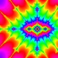
"Eye" of elephant resting on internal angle p/q of main cardioid = principal Misiurewicz point

Images edit

julia.tar
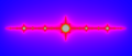
Mandelbrot set at Fibonacci point c = -1.8705286321646448888906
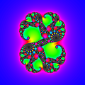
Airplane Julia set. C is the center of period 3 component on the real axis
Disconnected Julia set near period 16 component ( wake 1/16)
disconnected ( Cantor) Julia set from wake 1/19

kleinian.tar
Kleinian group limit set on sphere
Schottky (Kleinian) group limit set in plane

code edit

complex numbers edit

// from cx.c  programs by Curtis T McMullen
// http://www.math.harvard.edu/~ctm/programs/home/prog/julia/src/julia.tar

/* Compute sqrt(z) in the half-plane perpendicular to w. */
complex contsqrt(z,w)
complex z,w;
{
	complex cx_sqrt(), t;

	t = cx_sqrt(z);
	if (0 > (t.x*w.x + t.y*w.y)) 
		{t.x = -t.x; t.y = -t.y;}
	return(t);
}


/* Values in [-pi,pi]. */
double arg(z)  
	complex z;
{
	return(atan2(z.y,z.x));
}


complex cx_exp(z)
	complex z;
{
	complex w;
	double m;

	m = exp(z.x);
	w.x = m * cos(z.y);
	w.y = m * sin(z.y);
	return(w);
}

complex cx_log(z)
	complex z;
{
	complex w;

	w.x = log(cx_abs(z));
	w.y = arg(z);
	return(w);
}

complex cx_sin(z)
	complex z;
{
	complex w;

	w.x = sin(z.x) * cosh(z.y);
	w.y = cos(z.x) * sinh(z.y);
	return(w);
}

complex cx_cos(z)
	complex z;
{
	complex w;

	w.x = cos(z.x) * cosh(z.y);
	w.y = -sin(z.x) * sinh(z.y);
	return(w);
}

complex cx_sinh(z)
	complex z;
{
	complex w;

	w.x = sinh(z.x) * cos(z.y);
	w.y = cosh(z.x) * sin(z.y);
	return(w);
}

complex cx_cosh(z)
	complex z;
{
	complex w;

	w.x = cosh(z.x) * cos(z.y);
	w.y = sinh(z.x) * sin(z.y);
	return(w);
}

complex power(z,t)   /* Raise z to a real power t */
	complex z;
	double t;
{	double arg(), cx_abs(), pow();
	complex polar();

	return(polar(pow(cx_abs(z),t), t*arg(z)));
}

/*  Map points in the unit disk onto the lower hemisphere of the
    Riemann sphere by inverse stereographic projection.
    Projecting, r -> s = 2r/(r^2 + 1);  inverting this,
    s -> r = (1 - sqrt(1-s^2))/s.   */
 
complex disk_to_sphere(z)
	complex z;
{       complex w;
        double cx_abs(), r, s, sqrt();
 
        s = cx_abs(z);
        if (s == 0) return(z);
                else r = (1 - sqrt(1-s*s))/s;
        w.x = (r/s)*z.x;
        w.y = (r/s)*z.y;
        return(w);
}

complex mobius(a,b,c,d,z)
        complex a,b,c,d,z;

{       return(divide(add(mult(a,z),b),
                   add(mult(c,z),d)));
}

escape time and potential edit

// from quad.c  programs by Curtis T McMullen
// http://www.math.harvard.edu/~ctm/programs/home/prog/julia/src/julia.tar

/* F : \cx-K(f) -> {Re z > 0} is the multivalued
   function given by lim 2^{-n} log f^n(z).
   Re F(z) = rate, 
   (Re F(z))/|F'(z)| = dist.
   Returns 1 if z escaped, 0 otherwise.
*/

escape(z,c,iterlim,rate,dist)
	complex z,c;
	int iterlim;
	double *rate, *dist;
{
	int i;
	double fp, r, s;

	s = 1.0;
	fp = 1.0;
	for(i=0; i<iterlim; i++)
	{	r = cx_abs(z);
		if(r > LARGE)
		{	*rate = log(r)/s;
			*dist = r*log (r)/fp;
			return(1);
		}
		fp = fp * 2.0 * r;
		z = add(mult(z,z),c);
		s = s * 2.0;
	}
	return(0);
}

External ray edit

// from quad.c  programs by Curtis T McMullen
// http://www.math.harvard.edu/~ctm/programs/home/prog/julia/src/julia.tar

/* CAUTION is 2^{1/n} */
#define LOG2 .69314718055994530941
#define SQRT2 1.414213562373095
#define LARGE 200.0
#define LENGTH 200
#define CAUTION 0.9330329915368074
#define CIRCLEPTS 1000
#define EPS 0.000001
#define RAYEPS 1e-20
#define JFAC 1.0

/* Defaults */
#define C {0, 1}
#define CENTER {0.0,0.0}
#define RADIUS 1.5
#define PCLIM 0
#define SUBDIVIDE 8
#define ITERLIM 50  


/* Analytically continue Riemann mapping */
/* F : unit disk -> \cx-K(f) */
/* Assuming F(r,ang) is approx. z, find exact value*/

complex riemann(r,ang,z)
	double r;
	rational ang;
	complex z;
{
	complex orb[LENGTH], neworb[LENGTH];
	int i, n;

	orb[0] = z;
	n = 0;
	for (i=0; i<LENGTH-1; i++)
	{	if(cx_abs(orb[i]) > LARGE) break;
		orb[i+1] =
		add(mult(orb[i],orb[i]),c);
		n++;
		r = 2*r;
		ang.num = (2*ang.num)%ang.den;
	}
	neworb[n] = polar(pow(2.0,r),2*PIVAL*ang.num/ang.den);

	for(i=n; i>0; i--)
	{	neworb[i-1] =
		contsqrt(sub(neworb[i],c),orb[i-1]);
	}
	return(neworb[0]);
}


/* Set the color on a line joining z to w */
scan_line(z,w,col)
	complex z, w;
	int col;
{	
	int i, n;
	complex u;

	n = 4*cx_abs(sub(z,w))/pixrad;
	if(n == 0)
	{	scan_set(z,col);
		return;
	}
	for(i=0; i<=n; i++)
	{	u.x = (i*z.x + (n-i)*w.x)/n; 	
		u.y = (i*z.y + (n-i)*w.y)/n; 	
		scan_set(u,col);
	}
}


/* Draw an external ray */
draw_ray(level,ang)
	double level;
	rational ang;
{
	complex lastz, z;
	double r;

	r = level;
	while(pow(2.0,r) < LARGE) r *= 2;
	z = polar(pow(2.0,r),2*PIVAL*ang.num/ang.den);
	do
	{	r = r*CAUTION;
		lastz = z;
		z = riemann(r,ang,lastz);
		if(r < level*0.99) 
			scan_line(lastz,z,RAY);
	} while(r > RAYEPS);
}

Drawing dynamic external ray using inverse Boettcher map by Curtis McMullen edit

Julia set with external rays using McMullen method

This method is based on C program by Curtis McMullen^[3] and its Pascal version by Matjaz Erat^[4]

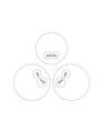
There are 2 planes^[5] here :

w-plane ( or f0 plane )
z-plane ( dynamic plane of fc plane )

Method consist of 3 big steps :

compute some w-points of external ray of circle for angle $\theta \,$ and various radii (rasterisation)

w_{0}=R*e^{2\pi it}\,

where

1<R<\infty \,

map w-points to z-point using inverse Boettcher map $\Psi _{c}=\Phi _{c}^{-1}\,$

z_{0}=\Psi _{c}(w_{0})=f_{c}^{-n}(w_{0}^{2^{n}})\,

draw z-points ( and connect them using segments ( line segment is a part of a line that is bounded by two distinct end points^[6] )

First and last steps are easy, but second is not so needs more explanation.

Rasterisation edit

For given external ray in $f_{0}\,$ plane each point of ray has :

constant value $t\,$ ( external angle in turns )
variable radius $R\,$

so $w\,$ points of ray are parametrised by radius $R\,$ and can be computed using exponential form of complex numbers :

w=F_{t}(R)=R*e^{2*\Pi *i*t}\,

One can go along ray using linear scale :

t:1/3; /* example value */
R_Max:4;
R_Min:1.1;
for R:R_Max step -0.5 thru R_Min do w:R*exp(2*%pi*%i*t);
/* Maxima allows non-integer values in for statement */

It gives some w points with equal distance between them.

Another method is to use nonlinera scale.

To do it we introduce floating point exponent $r\,$ such that :

R=2^{r}\,

and

w=G_{t}(r)=2^{r}*e^{2*\Pi *i*t}\,

To compute some w points of external ray in $f_{0}\,$ plane for angle $t\,$ use such Maxima code :

t:1/3; /* external angle in turns */
/* range for computing  R ; as r tends to 0 R tends to 1 */
rMax:2; /* so Rmax=2^2=4 /
rMin:0.1; /* rMin > 0   */
caution:0.93; /* positive number < 1 ; r:r*caution  gives smaller r */
r:rMax;
unless r<rMin do
( 
 r:r*caution, /* new smaller r */ 
 R:2^r, /* new smaller R */
 w:R*exp(2*%pi*%i*t) /* new point w in f0 plane */
);

In this method distance between points is not equal but inversely proportional to distance to boundary of filled Julia set.

It is good because here ray has greater curvature so curve will be more smooth.

Mapping edit

Mapping points from $f_{0}\,$ -plane to $f_{c}\,$ -plane consist of 4 minor steps :

forward iteration in $f_{0}\,$ plane

w_{n}=w_{0}^{2^{n}}=R^{2^{n}}*e^{2\pi i2^{n}t}\,

until $w_{n}\,$ is near infinity

abs(w_{n})>R_{limit}\,

switching plane ( from $f_{0}\,$ to $f_{c}\,$ )

z_{n}=w_{n}\,

( because here, near infinity : $w=z\,$ )

backward iteration in $f_{c}\,$ plane the same ( $n\,$ ) number of iterations
last point $z_{0}\,$ is on our external ray

1,2 and 4 minor steps are easy. Third is not.

z_{n-1}=f_{c}^{-1}(z_{n})={\sqrt {z_{n}-c}}\,

Backward iteration uses square root of complex number. It is 2-valued functions so backward iteration gives binary tree.

One can't choose good path in such tree without extre informations. To solve it we will use 2 things :

equicontinuity of basin of attraction of infinity
conjugacy between $f_{0}\,$ and $f_{c}\,$ planes

Equicontinuity of basin of attraction of infinity edit

Basin of attraction of infinity ( complement of filled-in Julia set) contains all points which tends to infinity under forward iteration.

$A_{f_{c}}(\infty )\ {\overset {\underset {\mathrm {def} }{}}{=}}\ \{z\in \mathbb {C} :f_{c}^{(k)}(z)\to \infty \ as\ k\to \infty \}.$

Infinity is superattracting fixed point and orbits of all points have similar behaviour. In other words orbits of 2 points are assumed to stay close if they are close at the beginning.

It is equicontinuity ( compare with normality).

In $f_{c}\,$ plane one can use forward orbit of previous point of ray for computing backward orbit of next point.

Detailed version of algorithm edit

compute first point of ray (start near infinity ang go toward Julia set )

w=2^{r}*e^{2\Pi it}\,

where

r=r_{max}\,

here one can easily switch planes :

z=w\,

It is our first z-point of ray.

compute next z-point of ray
- compute next w-point of ray for $r=r*caution\,$
- compute forward iteration of 2 points : previous z-point and actual w-point. Save z-orbit and last w-point
- switch planes and use last w-point as a starting point : $z_{n}=w_{last}\,$
- backward iteration of new $z_{n}\,$ toward new $z_{0}\,$ using forward orbit of previous z point
- $z_{0}\,$ is our next z point of our ray
and so on ( next points ) until $r<r_{Min}\,$

Maxima CAS src code

/* gives a list of z-points of external ray for angle t in turns and coefficient c */
GiveRay(t,c):=
block(
 [r],
 /* range for drawing  R=2^r ; as r tends to 0 R tends to 1 */
 rMin:1E-20, /* 1E-4;  rMin > 0  ; if rMin=0 then program has infinity loop !!!!! */
 rMax:2,  
 caution:0.9330329915368074, /* r:r*caution ; it gives smaller r */
 /* upper limit for iteration */
 R_max:300,
 /* */
 zz:[], /* array for z points of ray in fc plane */
 /*  some w-points of external ray in f0 plane  */
 r:rMax,
 while 2^r<R_max do r:2*r, /* find point w on ray near infinity (R>=R_max) in f0 plane */
 R:2^r,
 w:rectform(ev(R*exp(2*%pi*%i*t))),
 z:w, /* near infinity z=w */
 zz:cons(z,zz), 
 unless r<rMin do
 ( /* new smaller R */
  r:r*caution,  
  R:2^r,
  /* */
  w:rectform(ev(R*exp(2*%pi*%i*t))),
  /* */
  last_z:z,
  z:Psi_n(r,t,last_z,R_max), /* z=Psi_n(w) */
  zz:cons(z,zz)
 ),
 return(zz)
)$

Level curve of escape time edit

// from quad.c  programs by Curtis T McMullen
// http://www.math.harvard.edu/~ctm/programs/home/prog/julia/src/julia.tar

/* Color a level curve of escape */
draw_level(level)
	double level;
{
	double r;
	complex lastz, w, z;
	static rational zero={0,1};
	rational ang;

	r = level;
	while(pow(2.0,r) < LARGE) r *= 2;
	z = polar(pow(2.0,r),0.0);
	do
	{	r = r * CAUTION;
		lastz = z;
		z = riemann(r,zero,lastz);
	} while(r > level);

	lastz = z;
	ang.den = CIRCLEPTS;
	for(ang.num=0; ang.num<=CIRCLEPTS; ang.num++)
	{	z = riemann(level,ang,lastz);
		if(ang.num>0) scan_line(z,lastz,LEVEL);
		lastz = z;
	}
}

colors edit

// from quad.c  programs by Curtis T McMullen
// http://www.math.harvard.edu/~ctm/programs/home/prog/julia/src/julia.tar

/* Colors */
#define FILLED_JULIA 0
#define JULIA 1
#define PC_SET 2 
#define RAY 3
#define LEVEL 4
#define RESERVED 5
#define FREE (256-RESERVED)

set_gray(g)
	double g;
{
	int i;

	scan_gray(FILLED_JULIA,g);
	scan_gray(JULIA,0.0);
	scan_gray(PC_SET,0.0);
	scan_gray(RAY,0.0);
	scan_gray(LEVEL,0.0);
	for(i=0; i<FREE; i++)
		scan_gray(RESERVED+i,1.0);
}

set_colors()
{
	int i;

	scan_hls(FILLED_JULIA,0.0,70.0,0.0);
	scan_rgb(JULIA,0,0,0);
	scan_rgb(PC_SET,0,255,0);
	scan_rgb(RAY,0,0,0);
	scan_rgb(LEVEL,0,0,0);
	for(i=0; i<FREE; i++)
		scan_hls(RESERVED+i,
	((FREE-i)*360.0/FREE),50.0,100.0);
}

color(z)
	complex z;
{
	complex grad;
	double rate, dist;
	int i;

	if(escape(z,c,iterlim,&rate,&dist))
	{	if(dist < jfac*SQRT2*pixrad) 
			return(JULIA);
		i = subdivide * log(rate)/LOG2;
		while (i<0) i += FREE;
		return(RESERVED + i%FREE);
	}
	return(FILLED_JULIA);
}

// from scan.c  programs by Curtis T McMullen
// http://www.math.harvard.edu/~ctm/programs/home/prog/julia/src/julia.tar

scan_hls(i,h,l,s)
	int i;
	double h, l, s;
{
	int r, g, b;

	hlsrgb(h,l,s,&r,&g,&b);
	red[i] = r; green[i] = g; blue[i] = b;
	cmap = COLOR;
}



/* Convert hue/lightness/saturation to rgb */
/* Domain is [0,360] x [0,100] x [0,100]. */
/* Range is [0,255] x [0,255] x [0,255]. */

hlsrgb(h, l, s, r, g, b)
	double h, l, s;
	int *r, *g, *b;
{
	double M, m;
	double floor(), bound(), gun();

	h = h - floor(h/360) * 360;
	l = bound(0.0, l/100, 1.0);
	s = bound(0.0, s/100, 1.0);
	M = l + s*(l > 0.5 ? 1.0 - l : l);
	m = 2*l - M;
	*r = 255*gun(m, M, h);
	*g = 255*gun(m, M, h-120);
	*b = 255*gun(m, M, h-240);
}

double gun(m, M, h)
double m, M, h;
{
	if(h < 0)
		h += 360;
	if(h < 60)
		return(m + h*(M-m)/60);
	if(h < 180)
		return(M);
	if(h < 240)
		return(m + (240-h)*(M-m)/60);
	return(m);
}

double bound(low, x, high)
double low, x, high;
{
	if(x < low)
		return(low);
	if(x > high)
		return(high);
	return(x);
}

References edit

[1] rograms by Curtis T McMullen

[2] How to run programs

[3] rogram by Curtis McMullen (quad.c in Julia.tar.gz)

[4] Quadratische Polynome by Matjaz Erat

[5] wikipedia : Complex_quadratic_polynomial / planes / Dynamical_plane

[6] wikipedia : Line segment

[1]

[2]

[3]

[4]

[5]

[6]

Fractals/mcmullen

Contents