JPEG - Idea and Practice/The transform and quantization

The cosine transform

With the YCbCr representation of the colours, we can say that the picture is composed of three pictures of which the first is more significant than the two others. These three pictures are called the components of the picture: the Y component, the Cb component and the Cr component. But we can continue this process of getting few important and more less important elements. Let us assume that we have a picture in grey scale, then we can imagine that we start with a picture of only one colour, namely the average colour of all the colours in the picture, and by additions introduce more and more variation in the picture, so that at the end we have the complete picture. Then it would possibly turn out, that we could omit some of the last operations, as we were not able to distinguish the new additions. However, the expansion (which we have in mind) of the colour function in a sequence of terms having smaller and smaller importance, works only for a quadratic picture. Therefore our picture must be divided up in squares. And these squares must be rather small, because the number of calculations grows with the fourth power of the side length of the squares, which means that if the small squares are made twice as large, the number of calculations becomes four times as large. On the other hand, if the small squares are too small, the effect of the procedure is diminished. The optimal side length of the small squares seems to be 8-12 pixels. In JPEG the picture is divided up in 8x8-squares, but here we will see what happens if we let the squares have another side length than 8: we have arranged the program so that we can choose one of the numbers 2, 3, ..., 24 as side length s.

Thus, we perform a regular dividing up of the picture in sxs-squares. In JPEG this is done by starting at the left top corner and going from left to right line-wise from top to bottom, just as when we read a text. In our program for demonstration of the theory, we will however go through the picture in another way, namely column-wise from left to right and zigzagging down and up, so that the squares continually have a side in common. We will assume that the width and the height of the picture are divisible by s, or rather: we will only use the part of the picture lying within the largest domain (starting at the left top corner) which can be divided regularily up in sxs-squares. The method we use to expand the colour function within a square, is the discrete cosine transform (DCT) defined as follows.

We assume that we have a quadratic picture (in grey scales) of side length N, and we assume that N is rather large, so that we can talk about a "real" picture. This picture is a NxN-matrix of colour values (bytes): f(i, j), i, j = 0, 1, ..., N-1 (remember that (0, 0) corresponds to the left top corner, so that the ordinate j is measured downwards). We want to express f(i, j) in terms of pure double oscillations of the form f_{u, v}(i, j) = c(i, u) ∙ c(j, v), u, v = 0, ..., N-1, where the function c(i, u) is given by:

$c(i,u)=\cos {\frac {(2i+1)u\pi }{2N}}$

Note that f_{0, 0}(i, j) is constant 1 and that the function f_{u, v}(i, j) oscillates more the larger u or v are. We therefore want to express f(i, j) as a double sum of N² terms:

$f(i,j)=\sum _{u=0}^{N-1}\sum _{v=0}^{N-1}h(u,v)\cdot c(i,u)\cdot c(j,v)$

where the h(u, v)'s are (real) coefficients. The first term (u = 0 and v = 0) being a constant function is the average value of the N² numbers f(i, j). The following terms oscillate more and more (as functions of i and j), and if we omit some of the last terms, we get an approximation to f(i, j) that is free from the largest frequencies.

We can find the coefficients h(u, v) of this series expression of f(i, j) in the following way. Let the NxN-matrix (of real numbers) g(u, v) (u, v = 0, 1, ..., N-1) be defined by:

$g(u,v)={\frac {2\lambda (u)\lambda (v)}{N}}\sum _{i=0}^{N-1}\sum _{j=0}^{N-1}c(i,u)\cdot c(j,v)\cdot f(i,j)$

where λ(u) is 1 for u ≠ 0 and 1/√2 for u = 0. The matrix g(u, v) is called the (forward) discrete cosine transform (DCT or FDCT) of the matrix f(i, j). Note that g(0, 0) = N times the average of the colour values. There is a formula which, from the NxN-matrix g(u, v), brings us back to the original NxN-matrix f(i, j), and it has an analogue look:

f(i, j) = (2/N)∑_{u, v = 0, ..., N-1}λ(u)λ(v) ∙ c(i, u) ∙ c(j, v) ∙ g(u, v)

$f(i,j)={\frac {N}{2}}\sum _{u=0}^{N-1}\sum _{v=0}^{N-1}\lambda (u)\cdot \lambda (v)\cdot c(i,u)\cdot c(j,v)\cdot g(u,v)$

As this formula has the desired form for the series expansion of f(i, j), we see that the expansion is possible and that the coefficients h(u, v) are given by h(u, v) = (2λ(u)λ(v)/N) g(u, v). This formula for getting f(i, j) from g(u, v) is called the inverse discrete cosine transform (IDCT).

That the two formulas are inverse to each other, is easy to see if we take this formula, in which α and β are odd integers, for granted:

${\frac {1}{2}}\sum _{u=0}^{N-1}\cos {\frac {\alpha u\pi }{2N}}{\frac {\beta u\pi }{2N}}=0\;\;for\;\alpha \neq \beta \;and\;{\frac {N}{2}}for\;\alpha =\beta$

Now let us set N = 280, for instance, so that we consider a (grey scale) picture of 280x280 pixels. We transform the colour values f(i, j) (which are bytes), and from the transformed values g(u, v) (rounded off to integers which can be negative) we construct a picture, now in colours, because the numbers vary a lot and therefore cannot be measured in bytes. The new picture (also 280x280 pixels) could look like the picture to the left:

• 
  The cosine transformed picture
• 
  The reconstructed picture

After the transform, the "colour" values (in this example) vary from about -6000 to 24000, and the colouring is performed by a little trick: we have subtracted the minimum value from the values, so that they become non-negative, multiplied by (max - min)/65535 and rounded off, getting whole numbers from 0 to 65535 = 256² - 1. An integer in this interval can be written in the form a + 256xb, for bytes a and b, and to these we can associate the RGB triple (0, b, a), for instance (the numbers min and max must be introduced in the program which reconstructs the picture, but this can be done by writing them in some of the free entries in the header of the BMP file). The picture to the right above is the reconstructed picture.

If, in the reconstruction procedure, we remove the terms for u > N/2 or v > N/2, so that we only make use of the mean fourth of the terms, we get a picture that is almost as the original - only a little blurred:

• 
  All the terms
• 
  One fourth of the terms

However, in the JPEG procedure terms are not actually removed: the coefficients are replaced by approximations of whose those for the high frequencies can deviate more from the original coefficients than those for the low frequencies. It is in this way the quantization procedure is carried out.

Now to the (colour) picture divided up in small sxs-squares. After the cosine transform, we have s² numbers for each sxs-square and for each component (of the colour picture). From these numbers we can reconstruct the picture, and it is these numbers we are going to write in the file, after compressing. But if we did this without quantization (that is, without making the numbers numerically smaller in some way), we would have gained nothing by the cosine transform. Besides the quantization, to be explained below, we can do another thing which makes some of the values smaller and which has a good effect: we can replace each first term of the transformed values (the average value g(0, 0)) by its difference from the preceding first term of the same type (that is, for the preceding square for the same component). The first term g(0, 0) of the matrix g(u, v) (u, v = 0, ..., s-1) is called the DC term, and the others s²-1 terms, g(u, v), u > 0 or v > 0, are called the AC terms. Thus, we replace each of the DC terms (for a given sxs-square and component) by its derivation from the DC term of the preceding sxs-square (and the same component).

Quantization

Without the quantization procedure, the only source of loss of information would be rounding off of real numbers in order to get integers. As the mean numbers (g(u, v) for u or v near 0) are rather large, these errors are not significant: if we make the file now (that is, with cosine transform but without quantization) and apply a compression procedure (which is lossless), the picture which we can reconstruct from the file will be almost undistinguishable from the original, but it will still take up too much space. It is the quantization procedure that brings the size down and introduces deviations. By quantization we understand the procedure of making the coefficients of the expansion of f(i, j) in pure double oscillations, that is, the numbers g(u, v) from the cosine transform, smaller by dividing them by numbers q(u, v) depending on (u, v) and then rounding-off to integers. When the picture is to be drawn from the file, we multiply by the numbers we have divided by. If for instance g(u, v) = 135.6 is divided by q(u, v) = 36 and the result is rounded off, we get 4, and when we multiply 4 by 36, we get 144. We have then introduced errors which could be insignificant, since they are not errors in the colour values but in the cosine transformed numbers, and the main terms, the g(u, v)'s for u and v near 0, are quantized by much smaller numbers q(u, v) than the less important terms, the g(u, v)'s for u or v not near 0. Furthermore, as the numbers for the Y component have more significance than the numbers from the Cb and the Cr component, the cosine transformed numbers for these can bear to be quantized by larger numbers q(u, v).

The 8x8-matrices q(u, v) (u, v = 0, ..., 7) of the quantization numbers for the Y component and the two colour components used in the JPEG procedure are chosen according to experiments. Consequently, there are several bids for such tables. In part two you can see some typical tables. Well chosen numbers mean that we can compress more without damaging the picture, but we will always meet situations where a part of the picture has disturbing flaws that forces us to choose smaller quantization values. Usually a quality factor qf is introduced in the program that makes the file, so that the quantization numbers can be adjusted. For instance, we can arrange the dependence so that best possible quality - qf = 100 - means that there is no quantization (all the quantization numbers are set to 1), and that qf = 75 means that the given quantization table q(u, v) is used. The table q(u, v) and the quality factor qf are applied again when the picture is drawn from the file. The quality factor must of course appear in the header of the file, whereas the tables only need to be in the programs that produce the file and draw the picture.

In our program we must have quantization tables for varying side length of the small squares (from 2 to 24), and we must therefore construct the tables mathematically - as simple as possible. We first choose the q(u, v) values for qf = 75, and then find a formula so that all become 1 for qf = 100. Guided by the tables shown in part two, for qf = 75, we choose the following values for side length s and for the Y component and the colour components, respectively:

q(u, v) = (s/8)∙12∙(1 + 4∙√(u² + v²)/ s)

q(u, v) = (s/8)∙20∙(1 + 5∙√(u² + v²)/ s)

We arrange the program so that we can have different quality factors for the Y component and the colour components. We adjust the numbers q(u, v) according to qf in this way:

q(u, v)^{√(100 - qf)/5}

The left picture below (for side length s = 8) is without quantization (qf = 100), and the file takes up 60 per cent of the original BMP file. In the picture to the right qf = 70, and the file now takes up only 6 per cent of the original:

• 
  qf = 100
• 
  qf = 75

When we put the matrix of the quantization table and the matrix of the cosine transformed and quantized numbers into the file, we must arrange these numbers linearly in some way. We do this in such a way that the most important ones (those for u and v near 0) come first, namely by applying this zigzag principle:

• 
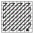  The zigzag principle

If s is the side length of the square, then the zigzag value m (= 1, 2, ..., s²) corresponding to the point (i, j) (i, j = 0, 1, ..., s-1) can be calculated with this program:

k = i + j
if k < s then
	begin
		l = (k * (k + 1)) div 2
		if k mod 2 = 0 then
			m = l + i + 1
		else
			m = l + j + 1
	end
if k = s then
	m = (s - 2) * (s - 2) + i
if k > s then
	begin
		k = 2 * s - 1 - k
		l = s * s - (k * (k + 1)) div 2
		if k mod 2 = 0 then
			m = l + (s - i)
		else
			m = l + (s - j)
	end