Haskell/Print version
| This is the print version of Haskell You won't see this message or any elements not part of the book's content when you print or preview this page. |
Table Of Contents
Haskell Basics
- Getting set up
- Variables and functions
- Truth values
- Type basics
- Lists and tuples
- Type basics II
- Next steps
- Building vocabulary
- Simple input and output
Elementary Haskell
- Recursion
- Lists II (map)
- Lists III (folds, comprehensions)
- Type declarations
- Pattern matching
- Control structures
- More on functions
- Higher-order functions
- Using GHCi effectively
Intermediate Haskell
- Modules
- Standalone programs
- Indentation
- More on datatypes
- Other data structures
- Classes and types
- The Functor class
Monads
- Prologue: IO, an applicative functor
- Understanding monads
- Maybe:List
donotation- IO:State
- Alternative and MonadPlus
- Monad transformers
Advanced Haskell
- Monoids
- Applicative functors
- Foldable
- Traversable
- Arrow tutorial
- Understanding arrows
- Continuation passing style
- Zippers
- Lenses
- Comonads
- Value recursion (MonadFix)
- Effectful streaming
- Mutable objects
- Concurrency
- Template Haskell
- Type Families
Fun with Types
- Polymorphism
- Existentially quantified types
- Advanced type classes
- Phantom types
- Generalised algebraic data-types (GADT)
- Datatype algebra
- Type constructors & Kinds
Wider Theory
- Denotational semantics
- Equational reasoning
- Program derivation
- Category theory
- The Curry–Howard isomorphism
- fix and recursion
Haskell Performance
- Introduction
- Step by step examples
- Graph reduction
- Laziness
- Time and space profiling
- Strictness
- Algorithm complexity
- Data structures
- Parallelism
Libraries Reference
General Practices
- Debugging
- Testing
- Packaging your software (Cabal)
- Using the Foreign Function Interface (FFI)
- Generic programming: Scrap your boilerplate
Specialised Tasks
- Graphical user interfaces (GUI)

- Databases

- Working with XML
- Parsing mathematical expressions

- Writing a basic type checker
Haskell Basics
Getting set up
Installing Haskell
Haskell is a programming language, i.e. a language in which humans can express how computers should behave. It's like writing a cooking recipe: you write the recipe and the computer executes it.
To use Haskell programs, you need a special program called a Haskell compiler. A compiler takes code written in Haskell and translates it into machine code, a more elementary language that the computer understands. Using the cooking analogy, you write a recipe (your Haskell program) and a cook (a compiler program) does the work of putting together actual ingredients into an edible dish (an executable file). Of course, you can't easily get the recipe from a final dish (and you can't get the Haskell code from the executable after it's compiled).
To get started, visit haskell.org/downloads for the latest instructions. The current recommended way is to use GHCup. Use it to install the latest recommended version of GHC, cabal (not stack), and the Haskell language server. You should use cabal to install any Haskell library you need. We will cover using cabal in depth in Haskell/Packaging
Note
Linux users:
It is heavily, heavily discouraged to install anything pertaining to Haskell using your system's package repositories and package manager (unless you're using Fedora or NixOS). Specifically distributions like Arch Linux and Debian manage Haskell packages very badly, and will lead to a bad experience with the tooling. Use GHCup and Cabal as noted above.
To just test some Haskell basics without downloading and installing, there is a playground which includes a few packages by default. Most instructions here on the Wikibook will also work on the playground, though it doesn't accept user input.
First code
After installation, we will do our first Haskell coding with the program called GHCi (the 'i' stands for 'interactive'). Depending on your operating system, perform the following steps:
- On Windows: Click Start, then Run, then type 'cmd' and hit Enter, then type
ghciand hit Enter once more. - On MacOS: Open the application "Terminal" found in the "Applications/Utilities" folder, type the letters
ghciinto the window that appears, and hit the Enter key. - On Linux: Open a terminal and run
ghci.
You should get output that looks something like the following:
GHCi, version 8.10.7: http://www.haskell.org/ghc/  :? for help
Prelude>
The first bit is GHCi's version, and tells your how to get help in GHCi. The Prelude> bit is known as the prompt. This is where you enter commands, and GHCi will respond with their results. The prompt also tells you that the current loaded module is Prelude, which gives you access to most of the built-in functions.
Now let's try some basic arithmetic:
Prelude> 2 + 2
4
Prelude> 5 + 4 * 3
17
Prelude> 2 ^ 5
32
These operators match most other programming languages: + is addition, * is multiplication, and ^ is exponentiation (raising to the power of, or ). As shown in the second example, Haskell follows standard order of math operations (e.g. multiplication before addition).

Now you know how to use Haskell as a calculator. Actually, Haskell is always a calculator — just a really powerful one, able to deal not only with numbers but also with other objects like characters, lists, functions, trees, and even other programs (if you aren't familiar with these terms yet, don't worry).
To leave GHCi once you are done, use :quit (or just :q):
Prelude> :quit
Leaving GHCi.
GHCi is a powerful development environment. As we progress, we will learn how to load files with source code into GHCi and evaluate different parts of them.
Assuming you're clear on everything so far (if not, use the talk page and help us improve this Wikibook!), then you are ready for next chapter where we will introduce some of the basic concepts of Haskell and make our first Haskell functions.
Variables and functions
All the examples in this chapter can be saved into a Haskell source file and then evaluated by loading that file into GHCi. Do not include the "Prelude>" prompts part of any example. When that prompt is shown, it means you can type the following code into an environment like GHCi. Otherwise, you should put the code in a file and run it.
Variables
In the last chapter, we used GHCi as a calculator. Of course, that's only practical for short calculations. For longer calculations and for writing Haskell programs, we want to keep track of intermediate results.
We can store intermediate results by assigning them names. These names are called variables. When a program runs, each variable is substituted for the value to which it refers. For instance, consider the following calculation:
Prelude> 3.141592653 * 5^2
78.539816325
That is the approximate area of a circle with radius 5, according to the formula . Of course, it is cumbersome to type in the digits of , or even to remember more than the first few. Programming helps us avoid mindless repetition and rote memorization by delegating these tasks to a machine. That way, our minds stay free to deal with more interesting ideas. For the present case, Haskell already includes a variable named pi that stores over a dozen digits of for us. This allows for not just clearer code, but also greater precision:


Prelude> pi
3.141592653589793
Prelude> pi * 5^2
78.53981633974483
Note that the variable pi and its value, 3.141592653589793, can be used interchangeably in calculations.
Haskell source files
Beyond momentary operations in GHCi, you will save your code in Haskell source files (basically plain text) with the extension .hs. Work with these files using a text editor appropriate for coding (see the Wikipedia article on text editors). Proper source code editors will provide syntax highlighting, which colors the code in relevant ways to make reading and understanding easier. Vim and Emacs are popular choices among Haskell programmers.
To keep things tidy, create a directory (i.e. a folder) in your computer to save the Haskell files you will create while doing the exercises in this book. Call the directory something like HaskellWikibook. Then, create a new file in that directory called Varfun.hs with the following code:
r = 5.0
That code defines the variable r as the value 5.0.
Note: make sure that there are no spaces at the beginning of the line because Haskell is sensitive to whitespace.
Next, with your terminal at the HaskellWikibook directory, start GHCi and load the Varfun.hs file using the :load command:
Prelude> :load Varfun.hs
[1 of 1] Compiling Main             ( Varfun.hs, interpreted )
Ok, modules loaded: Main.
Note that :load can be abbreviated as :l (as in :l Varfun.hs).
If GHCi gives an error like Could not find module 'Varfun.hs', you are probably running GHCi in the wrong directory or saved your file in the wrong directory. You can use the :cd command to change directories within GHCi (for instance, :cd HaskellWikibook).
With the file loaded, GHCi's prompt changes from "Prelude" to "*Main". You can now use the newly defined variable r in your calculations:
*Main> r
5.0
*Main> pi * r^2
78.53981633974483
So, we calculated the area of a circle with radius of 5.0 using the well-known formula . This worked because we defined r in our Varfun.hs file and pi comes from the standard Haskell libraries.

Next, we'll make the area formula easier to quickly access by defining a variable name for it. Change the contents of the source file to:
r = 5.0
area = pi * r ^ 2
Save the file. Then, assuming you kept GHCi running with the file still loaded, type :reload (or abbreviate version :r):
*Main> :reload
Compiling Main             ( Varfun.hs, interpreted )
Ok, modules loaded: Main.
*Main>
Now we have two variables r and area:
*Main> area
78.53981633974483
*Main> area / r
15.707963267948966
Note
The let keyword (a word with a special meaning) lets us define variables directly at the GHCi prompt without a source file. This looks like:
Prelude> let area = pi * 5 ^ 2
Although sometimes convenient, assigning variables entirely in GHCi this way is impractical for any complex tasks. We will usually want to use saved source files.
Comments
Besides the working code itself, source files may contain text comments. In Haskell there are two types of comment. The first starts with -- and continues until the end of the line:
x = 5     -- x is 5.
y = 6     -- y is 6.
-- z = 7  -- z is not defined.
In this case, x and y are defined in actual Haskell code, but z is not.
The second type of comment is denoted by an enclosing {- ... -} and can span multiple lines:
answer = 2 * {-
  block comment, crossing lines and...
  -} 3 {- inline comment. -} * 7
By combining single- and multi-line commenting, it is possible to toggle between executed and commented-out code by adding or removing a single } character, respectively:
{--
foo :: String
foo = "bar"
--}
vs.
{--}
foo :: String
foo = "bar"
--}
We use comments for explaining parts of a program or making other notes in context. Beware of comment overuse as too many comments can make programs harder to read. Also, we must carefully update comments whenever we change the corresponding code. Outdated comments can cause significant confusion.
Variables in imperative languages
Readers familiar with imperative programming will notice that variables in Haskell seem quite different from variables in languages like C. If you have no programming experience, you could skip this section, but it will help you understand the general situation when encountering the many cases (most Haskell textbooks, for example) where people discuss Haskell in reference to other programming languages.
Imperative programming treats variables as changeable locations in a computer's memory. That approach connects to the basic operating principles of computers. Imperative programs explicitly tell the computer what to do. Higher-level imperative languages are quite removed from direct computer assembly code instructions, but they retain the same step-by-step way of thinking. In contrast, functional programming offers a way to think in higher-level mathematical terms, defining how variables relate to one another, leaving the compiler to translate these to the step-by-step instructions that the computer can process.
Let's look at an example. The following code does not work in Haskell:
r = 5
r = 2
An imperative programmer may read this as first setting r = 5 and then changing it to r = 2. In Haskell, however, the compiler will respond to the code above with an error: "multiple declarations of r". Within a given scope, a variable in Haskell gets defined only once and cannot change.
The variables in Haskell seem almost invariable, but they work like variables in mathematics. In a math classroom, you never see a variable change its value within a single problem.
In precise terms, Haskell variables are immutable. They vary only based on the data we enter into a program. We can't define r two ways in the same code, but we could change the value by changing the file. Let's update our code from above:
r = 2.0
area = pi * r ^ 2
Of course, that works just fine. We can change r in the one place where it is defined, and that will automatically update the value of all the rest of the code that uses the r variable.
Real-world Haskell programs work by leaving some variables unspecified in the code. The values then get defined when the program gets data from an external file, a database, or user input. For now, however, we will stick to defining variables internally. We will cover interaction with external data in later chapters.
Here's one more example of a major difference from imperative languages:
r = r + 1
Instead of "incrementing the variable r" (i.e. updating the value in memory), this Haskell code is a recursive definition of r (i.e. defining it in terms of itself). We will explain recursion in detail later on. For this specific case, if r had been defined with any value beforehand, then r = r + 1 in Haskell would bring an error message. r = r + 1 is akin to saying, in a mathematical context, that , which is plainly wrong.

Because their values do not change within a program, variables can be defined in any order. For example, the following fragments of code do exactly the same thing:
 y = x * 2
 x = 3
|
 x = 3
 y = x * 2
|
In Haskell, there is no notion of "x being declared before y" or the other way around. Of course, using y will still require a value for x, but this is unimportant until you need a specific numeric value.
Functions
Changing our program every time we want to calculate the area of new circle is both tedious and limited to one circle at a time. We could calculate two circles by duplicating all the code using new variables r2 and area2 for the second circle:[1]
r  = 5
area  = pi * r ^ 2
r2 = 3
area2 = pi * r2 ^ 2
Of course, to eliminate this mindless repetition, we would prefer to have simply one function for area and then apply it to different radii.
A function takes an argument value (or parameter) and gives a result value (essentially the same as in mathematical functions). Defining functions in Haskell is like defining a variable, except that we take note of the function argument that we put on the left hand side of the equals sign. For instance, the following defines a function area which depends on an argument named r:
area r = pi * r ^ 2
Look closely at the syntax: the function name comes first (area in our example), followed by a space and then the argument (r in the example). Following the = sign, the function definition is a formula that uses the argument in context with other already defined terms.
Now, we can plug in different values for the argument in a call to the function. Save the code above in a file, load it into GHCi, and try the following:
*Main> area 5
78.53981633974483
*Main> area 3
28.274333882308138
*Main> area 17
907.9202768874502
Thus, we can call this function with different radii to calculate the area of any circle.
Our function here is defined mathematically as

In mathematics, the argument is enclosed between parentheses, as in or . Many programming languages likewise surround arguments with parentheses, as in max(2, 3). But Haskell omits parentheses around a list of arguments (as well as commas between them): max 2 3.


We still use parentheses for grouping expressions (any code that gives a value) that must be evaluated together. Note how the following expressions are parsed differently:
5 * 3 + 2       -- 15 + 2 = 17 (multiplication is done before addition)
5 * (3 + 2)     -- 5 * 5 = 25 (thanks to the parentheses)
area 5 * 3      -- (area 5) * 3
area (5 * 3)    -- area 15
Note that Haskell functions take precedence over all other operators such as + and *, in the same way that, for instance, multiplication is done before addition in mathematics.
Evaluation
What exactly happens when you enter an expression into GHCi? After you press the enter key, GHCi will evaluate the expression you have given. That means it will replace each function with its definition and calculate the results until a single value remains. For example, the evaluation of area 5 proceeds as follows:
   area 5
=>    { replace the left-hand side  area r = ...  by the right-hand side  ... = pi * r^2 }
   pi * 5 ^ 2
=>    { replace  pi  by its numerical value }
   3.141592653589793 * 5 ^ 2
=>    { apply exponentiation (^) }
   3.141592653589793 * 25
=>    { apply multiplication (*) }
   78.53981633974483
As this shows, to apply or call a function means to replace the left-hand side of its definition by its right-hand side. When using GHCi, the results of a function call will then show on the screen.
Some more functions:
double x    = 2 * x
quadruple x = double (double x)
square x    = x * x
half   x    = x / 2
| Exercises |
|---|
|
Multiple parameters
Functions can also take more than one argument. For example, a function for calculating the area of a rectangle given its length and width:
areaRect l w = l * w
*Main> areaRect 5 10
50
Another example that calculates the area of a triangle :

areaTriangle b h = (b * h) / 2
*Main> areaTriangle 3 9
13.5
As you can see, multiple arguments are separated by spaces. That's also why you sometimes have to use parentheses to group expressions. For instance, to quadruple a value x, you can't write:
quadruple x = double double x -- error
That would apply a function named double to the two arguments double and x. Note that functions can be arguments to other functions (you will see why later). To make this example work, we need to put parentheses around the argument:
quadruple x = double (double x)
Arguments are always passed in the order given. For example:
minus x y = x - y
*Main> minus 10 5
5
*Main> minus 5 10
-5
Here, minus 10 5 evaluates to 10 - 5, but minus 5 10 evaluates to 5 - 10 because the order changes.
| Exercises |
|---|
|
On combining functions
Of course, you can use functions that you have already defined to define new functions, just like you can use the predefined functions like addition (+) or multiplication (*) (operators are defined as functions in Haskell). For example, to calculate the area of a square, we can reuse our function that calculates the area of a rectangle:
areaRect l w = l * w
areaSquare s = areaRect s s
*Main> areaSquare 5
25
After all, a square is just a rectangle with equal sides.
| Exercises |
|---|
|
Local definitions
where clauses
When defining a function, we sometimes want to define intermediate results that are local to the function. For instance, consider Heron's formula for calculating the area of a triangle with sides a, b, and c:

heron a b c = sqrt (s * (s - a) * (s - b) * (s - c))
    where
    s = (a + b + c) / 2
The variable s is half the perimeter of the triangle and it would be tedious to write it out four times in the argument of the square root function sqrt.
Simply writing the definitions in sequence does not work...
heron a b c = sqrt (s * (s - a) * (s - b) * (s - c))
s = (a + b + c) / 2                                   -- a, b, and c are not defined here
... because the variables a, b, c are only available in the right-hand side of the function heron, but the definition of s as written here is not part of the right-hand side of heron. To make it part of the right-hand side, we use the where keyword.
Note that both the where and the local definitions are indented by 4 spaces, to distinguish them from subsequent definitions. Here is another example that shows a mix of local and top-level definitions:
areaTriangleTrig  a b c = c * height / 2   -- use trigonometry
    where
    cosa   = (b ^ 2 + c ^ 2 - a ^ 2) / (2 * b * c)
    sina   = sqrt (1 - cosa ^ 2)
    height = b * sina
areaTriangleHeron a b c = result           -- use Heron's formula
    where
    result = sqrt (s * (s - a) * (s - b) * (s - c))
    s      = (a + b + c) / 2
Scope
If you look closely at the previous example, you'll notice that we have used the variable names a, b, c twice, once for each of the two area functions. How does that work?
Consider the following GHCi sequence:
Prelude> let r = 0
Prelude> let area r = pi * r ^ 2
Prelude> area 5
78.53981633974483
It would have been an unpleasant surprise to return 0 for the area because of the earlier let r = 0 definition getting in the way. That does not happen because when you defined r the second time you are talking about a different r. This may seem confusing, but consider how many people have the name John, and yet for any context with only one John, we can talk about "John" with no confusion. Programming has a notion similar to context, called scope.
We will not explain the technicalities behind scope right now. Just keep in mind that the value of a parameter is strictly what you pass in when you call the function, regardless of what the variable was called in the function's definition. That said, appropriately unique names for variables do make the code easier for human readers to understand.
Summary
- Variables store values (which can be any arbitrary Haskell expression).
- Variables do not change within a scope.
- Functions help you write reusable code.
- Functions can accept more than one parameter.
We also learned about non-code text comments within a source file.
Notes
- ↑ As this example shows, the names of variables may contain numbers as well as letters. Variables in Haskell must begin with a lowercase letter but may then have any string consisting of letter, numbers, underscore (_) or tick (').
Truth values
Equality and other comparisons
In the last chapter, we used the equals sign to define variables and functions in Haskell as in the following code:
r = 5
That means that the evaluation of the program replaces all occurrences of r with 5 (within the scope of the definition). Similarly, evaluating the code
f x = x + 3
replaces all occurrences of f followed by a number (f's argument) with that number plus three.
Mathematics also uses the equals sign in an important and subtly different way. For instance, consider this simple problem:
Example: Solve the following equation:

Our interest here isn't about representing the value as , or vice-versa. Instead, we read the equation as a proposition that some number gives 5 as result when added to 3. Solving the equation means finding which, if any, values of make that proposition true. In this example, elementary algebra tells us that (i.e. 2 is the number that will make the equation true, giving ).


Comparing values to see if they are equal is also useful in programming. In Haskell, such tests look just like an equation. Since the equals sign is already used for defining things, Haskell uses a double equals sign, == instead. Enter our proposition above in GHCi:
Prelude> 2 + 3 == 5
True
GHCi returns "True" because is equal to 5. What if we use an equation that is not true?

Prelude> 7 + 3 == 5
False
Nice and coherent. Next, we will use our own functions in these tests. Let's try the function f we mentioned at the start of the chapter:
Prelude> let f x = x + 3
Prelude> f 2 == 5
True
This works as expected because f 2 evaluates to 2 + 3.
We can also compare two numerical values to see which one is larger. Haskell provides a number of tests including: < (less than), > (greater than), <= (less than or equal to) and >= (greater than or equal to). These tests work comparably to == (equal to). For example, we could use < alongside the area function from the previous module to see whether a circle of a certain radius would have an area smaller than some value.
Prelude> let area r = pi * r ^ 2
Prelude> area 5 < 50
False
Boolean values
What is actually going on when GHCi determines whether these arithmetical propositions are true or false? Consider a different but related issue. If we enter an arithmetical expression in GHCi the expression gets evaluated, and the resulting numerical value is displayed on the screen:
Prelude> 2 + 2
4
If we replace the arithmetical expression with an equality comparison, something similar seems to happen:
Prelude> 2 == 2
True
Whereas the "4" returned earlier is a number which represents some kind of count, quantity, etc., "True" is a value that stands for the truth of a proposition. Such values are called truth values, or boolean values.[1] Naturally, only two possible boolean values exist: True and False.
Introduction to types
True and False are real values, not just an analogy. Boolean values have the same status as numerical values in Haskell, and you can manipulate them in similar ways. One trivial example:
Prelude> True == True
True
Prelude> True == False
False
True is indeed equal to True, and True is not equal to False. Now: can you answer whether 2 is equal to True?
Prelude> 2 == True

<interactive>:1:0:
    No instance for (Num Bool)
      arising from the literal ‘2’ at <interactive>:1:0
    Possible fix: add an instance declaration for (Num Bool)
    In the first argument of ‘(==)’, namely ‘2’
    In the expression: 2 == True
    In an equation for ‘it’: it = 2 == True
Error! The question just does not make sense. We cannot compare a number with a non-number or a boolean with a non-boolean. Haskell incorporates that notion, and the ugly error message complains about this. Ignoring much of the clutter, the message says that there was a number (Num) on the left side of the ==, and so some kind of number was expected on the right side; however, a boolean value (Bool) is not a number, and so the equality test failed.
So, values have types, and these types define limits to what we can or cannot do with the values. True and False are values of type Bool. The 2 is complicated because there are many different types of numbers, so we will defer that explanation until later. Overall, types provide great power because they regulate the behavior of values with rules that make sense, making it easier to write programs that work correctly. We will come back to the topic of types many times as they are very important to Haskell.
Infix operators
An equality test like 2 == 2 is an expression just like 2 + 2; it evaluates to a value in pretty much the same way. The ugly error message we got on the previous example even says so:
In the expression: 2 == True
When we type 2 == 2 in the prompt and GHCi "answers" True, it is simply evaluating an expression. In fact, == is itself a function which takes two arguments (which are the left side and the right side of the equality test), but the syntax is notable: Haskell allows two-argument functions to be written as infix operators placed between their arguments. When the function name uses only non-alphanumeric characters, this infix approach is the common use case. If you wish to use such a function in the "standard" way (writing the function name before the arguments, as a prefix operator) the function name must be enclosed in parentheses. So the following expressions are completely equivalent:
Prelude> 4 + 9 == 13
True
Prelude> (==) (4 + 9) 13
True
Thus, we see how (==) works as a function similarly to areaRect from the previous module. The same considerations apply to the other relational operators we mentioned (<, >, <=, >=) and to the arithmetical operators (+, *, etc.) – all are functions that take two arguments and are normally written as infix operators.
In general, we can say that tangible things in Haskell are either values or functions.
Boolean operations
Haskell provides three basic functions for further manipulation of truth values as in logic propositions:
(&&)performs the and operation. Given two boolean values, it evaluates toTrueif both the first and the second areTrue, and toFalseotherwise.
Prelude> (3 < 8) && (False == False)
True
Prelude> (&&) (6 <= 5) (1 == 1)
False
(||)performs the or operation. Given two boolean values, it evaluates toTrueif at least one of them isTrueand toFalseotherwise.
Prelude> (2 + 2 == 5) || (2 > 0)
True
Prelude> (||) (18 == 17) (9 >= 11)
False
notperforms the negation of a boolean value; that is, it convertsTruetoFalseand vice-versa.
Prelude> not (5 * 2 == 10)
False
Haskell libraries already include the relational operator function (/=) for not equal to, but we could easily implement it ourselves as:
x /= y = not (x == y)
Note that we can write operators infix even when defining them. Completely new operators can also be created out of ASCII symbols (which means mostly the common symbols used on a keyboard).
Guards
Haskell programs often use boolean operators in convenient and abbreviated syntax. When the same logic is written in alternative styles, we call this syntactic sugar because it sweetens the code from the human perspective. We'll start with guards, a feature that relies on boolean values and allows us to write simple but powerful functions.
Let's implement the absolute value function. The absolute value of a real number is the number with its sign discarded; so if the number is negative (that is, smaller than zero) the sign is inverted; otherwise it remains unchanged. We could write the definition as:

Here, the actual expression to be used for calculating depends on a set of propositions made about . If is true, then we use the first expression, but if is the case, then we use the second expression instead. To express this decision process in Haskell using guards, the implementation could look like this:[2]


Example: The absolute value function.
absolute x
    | x < 0     = -x
    | otherwise = x
Remarkably, the above code is about as readable as the corresponding mathematical definition. Let us dissect the components of the definition:
- We start just like a normal function definition, providing a name for the function,
absolute, and saying it will take a single argument, which we will namex.
- Instead of just following with the
=and the right-hand side of the definition, we enter the two alternatives placed below on separate lines.[3] These alternatives are the guards proper. Note that the whitespace (the indentation of the second and third lines) is not just for aesthetic reasons; it is necessary for the code to be parsed correctly.
- Each of the guards begins with a pipe character,
|. After the pipe, we put an expression which evaluates to a boolean (also called a boolean condition or a predicate), which is followed by the rest of the definition. The function only uses the equals sign and the right-hand side from a line if the predicate evaluates toTrue.
- The
otherwisecase is used when none of the preceding predicates evaluate toTrue. In this case, ifxis not smaller than zero, it must be greater than or equal to zero, so the final predicate could have just as easily beenx >= 0; butotherwiseworks just as well.
Note
There is no syntactical magic behind otherwise. It is defined alongside the default variables and functions of Haskell as simply
otherwise = True
This definition makes otherwise a catch-all guard. As evaluation of the guard predicates is sequential, the otherwise predicate will only be reached if none of the previous cases evaluate to True (so make sure you always place otherwise as the last guard!). In general, it is a good idea to always provide an otherwise guard, because a rather ugly runtime error will be produced if none of the predicates is true for some input.
Note
In the first guard
| x < 0 = -x
we used the minus sign to negate x. It is worth noting that this way of expressing sign inversion is a special case of sorts, in that the - is not a function that takes one argument and evaluates to 0 - x, but merely a syntactical abbreviation. While very handy, this abbreviation occasionally conflicts with the usage of (-) as an actual function (the subtraction operator), which is a potential source of annoyance (for example, try writing three minus negative-four without using any parentheses for grouping).
That being so, when testing absolute with negative numbers you should call it like this:
Prelude> absolute (-10)
10
where and Guards
where clauses work well along with guards. For instance, consider a function which computes the number of (real) solutions for a quadratic equation, :

numOfRealSolutions a b c
    | disc > 0  = 2
    | disc == 0 = 1
    | otherwise = 0
        where
        disc = b^2 - 4*a*c
The where definition is within the scope of all of the guards, sparing us from repeating the expression for disc.
Notes
- ↑ The term is a tribute to the mathematician and philosopher George Boole.
- ↑ This function is already provided by Haskell with the name
abs, so in a real-world situation you don't need to provide an implementation yourself. - ↑ We could have joined the lines and written everything in a single line, but it would be less readable.
Type basics
In programming, Types are used to group similar values into categories. In Haskell, the type system is a powerful way of reducing the number of mistakes in your code.
Introduction
Programming deals with different sorts of entities. For example, consider adding two numbers together:
What are 2 and 3? Well, they are numbers. What about the plus sign in the middle? That's certainly not a number, but it stands for an operation which we can do with two numbers – namely, addition.
Similarly, consider a program that asks you for your name and then greets you with a "Hello" message. Neither your name nor the word Hello are numbers. What are they then? We might refer to all words and sentences and so forth as text. It's normal in programming to use a slightly more esoteric word: String, which is short for "string of characters".
Databases illustrate clearly the concept of types. For example, say we had a table in a database to store details about a person's contacts; a kind of personal telephone book. The contents might look like this:
| First Name | Last Name | Address | Telephone number |
| Sherlock | Holmes | 221B Baker Street London | 743756 |
| Bob | Jones | 99 Long Road Street Villestown | 655523 |
The fields in each entry contain values. Sherlock is a value as is 99 Long Road Street Villestown as well as 655523. Let's classify the values in this example in terms of types. "First Name" and "Last Name" contain text, so we say that the values are of type String.
At first glance, we might classify address as a String. However, the semantics behind an innocent address are quite complex. Many human conventions dictate how we interpret addresses. For example, if the beginning of the address text contains a number it is likely the number of the house. If not, then it's probably the name of the house – except if it starts with "PO Box", in which case it's just a postal box address and doesn't indicate where the person lives at all. Each part of the address has its own meaning.
In principle, we can indeed say that addresses are Strings, but that doesn't capture many important features of addresses. When we describe something as a String, all that we are saying is that it is a sequence of characters (letters, numbers, etc). Recognizing something as a specialized type is far more meaningful. If we know something is an Address, we instantly know much more about the piece of data – for instance, that we can interpret it using the "human conventions" that give meaning to addresses.
We might also apply this rationale to the telephone numbers. We could specify a TelephoneNumber type. Then, if we were to come across some arbitrary sequence of digits which happened to be of type TelephoneNumber we would have access to a lot more information than if it were just a Number – for instance, we could start looking for things such as area and country codes on the initial digits.
Another reason not to consider the telephone numbers as Numbers is that doing arithmetic with them makes no sense. What is the meaning and expected effect of, say, multiplying a TelephoneNumber by 100? It would not allow calling anyone by phone. Also, each digit comprising a telephone number is important; we cannot accept losing some of them by rounding or even by omitting leading zeros.
Why types are useful
How does it help us program well to describe and categorize things? Once we define a type, we can specify what we can or cannot do with it. That makes it far easier to manage larger programs and avoid errors.
Using the interactive :type command
Let's explore how types work using GHCi. The type of any expression can be checked with :type (or shortened to :t) command. Try this on the boolean values from the previous module:
Example: Exploring the types of boolean values in GHCi
Prelude> :type True
True :: Bool
Prelude> :type False
False :: Bool
Prelude> :t (3 < 5)
(3 < 5) :: Bool
The symbol ::, which will appear in a couple other places, can be read as simply "is of type", and indicates a type signature.
:type reveals that truth values in Haskell are of type Bool, as illustrated above for the two possible values, True and False, as well as for a sample expression that will evaluate to one of them. Note that boolean values are not just for value comparisons. Bool captures the semantics of a yes/no answer, so it can represent any information of such kind – say, whether a name was found in a spreadsheet, or whether a user has toggled an on/off option.
Characters and strings
Now let's try :t on something new. Literal characters are entered by enclosing them with single quotation marks. For instance, this is the single letter H:
Example: Using the :type command in GHCi on a literal character
Prelude> :t 'H'
'H' :: Char
So, literal character values have type Char (short for "character"). Now, single quotation marks only work for individual characters, so if we need to enter longer text – that is, a string of characters – we use double quotation marks instead:
Example: Using the :t command in GHCi on a literal string
Prelude> :t "Hello World"
"Hello World" :: [Char]
Why did we get Char again? The difference is the square brackets. [Char] means a number of characters chained together, forming a list of characters. Haskell considers all Strings to be lists of characters. Lists in general are important entities in Haskell, and we will cover them in more detail in a little while.
| Exercises |
|---|
|
Incidentally, Haskell allows for type synonyms, which work pretty much like synonyms in human languages (words that mean the same thing – say, 'big' and 'large'). In Haskell, type synonyms are alternative names for types. For instance, String is defined as a synonym of [Char], and so we can freely substitute one with the other. Therefore, to say:
"Hello World" :: String
is also perfectly valid, and in many cases a lot more readable. From here on we'll mostly refer to text values as String, rather than [Char].
Functional types
So far, we have seen how values (strings, booleans, characters, etc.) have types and how these types help us to categorize and describe them. Now, the big twist that makes Haskell's type system truly powerful: Functions have types as well.[1] Let's look at some examples to see how that works.
Example: not
We can negate boolean values with not (e.g. not True evaluates to False and vice-versa). To figure out the type of a function, we consider two things: the type of values it takes as its input and the type of value it returns. In this example, things are easy. not takes a Bool (the Bool to be negated), and returns a Bool (the negated Bool). The notation for writing that down is:
Example: Type signature for not
not :: Bool -> Bool
You can read this as "not is a function from things of type Bool to things of type Bool".
Using :t on a function will work just as expected:
Prelude> :t not
not :: Bool -> Bool
The description of a function's type is in terms of the types of argument(s) it takes and the type of value it evaluates to.
Example: chr and ord
Text presents a problem to computers. At its lowest level, a computer only knows binary 1s and 0s. To represent text, every character is first converted to a number, then that number is converted to binary and stored. That's how a piece of text (which is just a sequence of characters) is encoded into binary. Normally, we're only interested in how to encode characters into their numerical representations, because the computer takes care of the conversion to binary numbers without our intervention.
The easiest way to convert characters to numbers is simply to write all the possible characters down, then number them. For example, we might decide that 'a' corresponds to 1, then 'b' to 2, and so on. This is what something called the ASCII standard is: take 128 commonly-used characters and number them (ASCII doesn't actually start with 'a', but the general idea is the same). Of course, it would be quite a chore to sit down and look up a character in a big lookup table every time we wanted to encode it, so we've got two functions that do it for us, chr (pronounced 'char') and ord[2]:
Example: Type signatures for chr and ord
chr :: Int  -> Char
ord :: Char -> Int
We already know what Char means. The new type on the signatures above, Int, refers to integer numbers, and is one of quite a few different types of numbers.[3] The type signature of chr tells us that it takes an argument of type Int, an integer number, and evaluates to a result of type Char. The converse is the case with ord: It takes things of type Char and returns things of type Int. With the info from the type signatures, it becomes immediately clear which of the functions encodes a character into a numeric code (ord) and which does the decoding back to a character (chr).
To make things more concrete, here are a few examples. Notice that the two functions aren't available by default; so before trying them in GHCi you need to use the :module Data.Char (or :m Data.Char) command to load the Data.Char module where they are defined.
Example: Function calls to chr and ord
Prelude> :m Data.Char
Prelude Data.Char> chr 97
'a'
Prelude Data.Char> chr 98
'b'
Prelude Data.Char> ord 'c'
99
Functions with more than one argument
What would be the type of a function that takes more than one argument?
Example: A function with more than one argument
xor p q = (p || q) && not (p && q)
(xor is the exclusive-or function, which evaluates to True if either one or the other argument is True, but not both; and False otherwise.)
The general technique for forming the type of a function that accepts more than one argument is simply to write down all the types of the arguments in a row, in order (so in this case p first then q), then link them all with ->. Finally, add the type of the result to the end of the row and stick a final -> in just before it.[4] In this example, we have:
-
Write down the types of the arguments. In this case, the use of
(||)and(&&)gives away thatpandqhave to be of typeBool:Bool Bool ^^ p is a Bool ^^ q is a Bool as well
- Fill in the gaps with
->:Bool -> Bool
- Add in the result type and a final
->. In our case, we're just doing some basic boolean operations so the result remains a Bool.Bool -> Bool -> Bool ^^ We're returning a Bool ^^ This is the extra -> that got added in
The final signature, then, is:
Example: The signature of xor
xor :: Bool -> Bool -> Bool
Real world example: openWindow
As you'll learn in the Haskell in Practice section of the course, one popular group of Haskell libraries are the GUI (Graphical User Interface) ones. These provide functions for dealing with the visual things computer users are familiar with: menus, buttons, application windows, moving the mouse around, etc. One function from one of these libraries is called openWindow, and you can use it to open a new window in your application. For example, say you're writing a word processor, and the user has clicked on the 'Options' button. You need to open a new window which contains all the options that they can change. Let's look at the type signature for this function:[5]
Example: openWindow
openWindow :: WindowTitle -> WindowSize -> Window
You don't know these types, but they're quite simple. All three of the types there, WindowTitle, WindowSize and Window are defined by the GUI library that provides openWindow. As we saw earlier, the two arrows mean that the first two types are the types of the parameters, and the last is the type of the result. WindowTitle holds the title of the window (which typically appears in a title bar at the very top of the window), and WindowSize specifies how big the window should be. The function then returns a value of type Window which represents the actual window.
So, even if you have never seen a function before or don't know how it actually works, a type signature can give you a general idea of what the function does. Make a habit of testing every new function you meet with :t. If you start doing that now, you'll not only learn about the standard library Haskell functions but also develop a useful kind of intuition about functions in Haskell.
| Exercises |
|---|
|
What are the types of the following functions? For any functions involving numbers, you can just pretend the numbers are Ints.
|
Type signatures in code
We have explored the basic theory behind types and how they apply to Haskell. Now, we will see how type signatures are used for annotating functions in source files. Consider the xor function from an earlier example:
Example: A function with its signature
xor :: Bool -> Bool -> Bool
xor p q = (p || q) && not (p && q)
That is all we have to do. For maximum clarity, type signatures go above the corresponding function definition.
The signatures we add in this way serve a dual role: they clarify the type of the functions both to human readers and to the compiler/interpreter.
Type inference
If type signatures tell the interpreter (or compiler) about the function type, how did we write our earliest Haskell code without type signatures? Well, when you don't tell Haskell the types of your functions and variables it figures them out through a process called type inference. In essence, the compiler starts with the types of things it knows and then works out the types of the rest of the values. Consider a general example:
Example: Simple type inference
-- We're deliberately not providing a type signature for this function
isL c = c == 'l'
isL is a function that takes an argument c and returns the result of evaluating c == 'l'. Without a type signature, the type of c and the type of the result are not specified. In the expression c == 'l', however, the compiler knows that 'l' is a Char. Since c and 'l' are being compared with equality with (==) and both arguments of (==) must have the same type,[6] it follows that c must be a Char. Finally, since isL c is the result of (==) it must be a Bool. And thus we have a signature for the function:
Example: isL with a type
isL :: Char -> Bool
isL c = c == 'l'
Indeed, if you leave out the type signature, the Haskell compiler will discover it through this process. You can verify that by using :t on isL with or without a signature.
So why write type signatures if they will be inferred anyway? In some cases, the compiler lacks information to infer the type, and so the signature becomes obligatory. In some other cases, we can use a type signature to influence to a certain extent the final type of a function or value. These cases needn't concern us for now, but we have a few other reasons to include type signatures:
- Documentation: type signatures make your code easier to read. With most functions, the name of the function along with the type of the function is sufficient to guess what the function does. Of course, commenting your code helps, but having the types clearly stated helps too.
- Debugging: when you annotate a function with a type signature and then make a typo in the body of the function which changes the type of a variable, the compiler will tell you, at compile-time, that your function is wrong. Leaving off the type signature might allow your erroneous function to compile, and the compiler would assign it the wrong type. You wouldn't know until you ran your program that you made this mistake.
Types and readability
A somewhat more realistic example will help us understand better how signatures can help documentation. The piece of code quoted below is a tiny module (modules are the typical way of preparing a library), and this way of organizing code is like that in the libraries bundled with GHC.
Note
Do not go crazy trying to understand how the functions here actually work; that is beside the point as we still have not covered many of the features being used. Just keep reading and play along.
Example: Module with type signatures
module StringManip where

import Data.Char

uppercase, lowercase :: String -> String
uppercase = map toUpper
lowercase = map toLower

capitalize :: String -> String
capitalize x =
  let capWord []     = []
      capWord (x:xs) = toUpper x : xs
  in unwords (map capWord (words x))
This tiny library provides three string manipulation functions. uppercase converts a string to upper case, lowercase to lower case, and capitalize capitalizes the first letter of every word. Each of these functions takes a String as argument and evaluates to another String. Even if we do not understand how these functions work, looking at the type signatures allows us to immediately know the types of the arguments and return values. Paired with sensible function names, we have enough information to figure out how we can use the functions.
Note that when functions have the same type we have the option of writing just one signature for all of them, by separating their names with commas, as above with uppercase and lowercase.
Types prevent errors
The role of types in preventing errors is central to typed languages. When passing expressions around you have to make sure the types match up like they did here. If they don't, you'll get type errors when you try to compile; your program won't pass the typecheck. This helps reduce bugs in your programs. To take a very trivial example:
Example: A non-typechecking program
"hello" + " world" -- type error
That line will cause a program to fail when compiling. You can't add two strings together. In all likelihood, the programmer intended to use the similar-looking concatenation operator, which can be used to join two strings together into a single one:
Example: Our erroneous program, fixed
"hello" ++ " world" -- "hello world"
An easy typo to make, but Haskell catches the error when you tried to compile. You don't have to wait until you run the program for the bug to become apparent.
Updating a program commonly involves changes to types. If a change is unintended, or has unforeseen consequences, then it will show up when compiling. Haskell programmers often remark that once they have fixed all the type errors, and their programs compile, that they tend to "just work". The behavior may not always match the intention, but the program won't crash. Haskell has far fewer run-time errors (where your program goes wrong when you run it rather than when you compile) than other languages.
Notes
- ↑ The deeper truth is that functions are values, just like all the others.
- ↑ This isn't quite what
chrandorddo, but that description fits our purposes well, and it's close enough. - ↑ In fact, it is not even the only type for integers! We will meet its relatives in a short while.
- ↑ This method might seem just a trivial hack by now, but actually there are very deep reasons behind it, which we'll cover in the chapter on higher-order functions.
- ↑ This has been somewhat simplified to fit our purposes. Don't worry, the essence of the function is there.
- ↑ As discussed in Truth values. That fact is actually stated by the type signature of
(==)– if you are curious you can check it, although you will have to wait a little bit more for a full explanation of the notation used in that.
Lists and tuples
Haskell uses two fundamental structures for managing several values: lists and tuples. They both work by grouping multiple values into a single combined value.
Lists
Let's build some lists in GHCi:
Prelude> let numbers = [1,2,3,4]
Prelude> let truths  = [True, False, False]
Prelude> let strings = ["here", "are", "some", "strings"]
The square brackets delimit the list, and individual elements are separated by commas. The only important restriction is that all elements in a list must be of the same type. Trying to define a list with mixed-type elements results in a typical type error:
Prelude> let mixed = [True, "bonjour"]

<interactive>:1:19:
    Couldn't match `Bool' against `[Char]'
      Expected type: Bool
      Inferred type: [Char]
    In the list element: "bonjour"
    In the definition of `mixed': mixed = [True, "bonjour"]
Building lists
In addition to specifying the whole list at once using square brackets and commas, you can build them up piece by piece using the (:) operator pronounced "cons". The process of building up a list this way is often referred to as consing. This terminology comes from LISP programmers who invented the verb "to cons" (a mnemonic for "constructor") to refer to this specific task of prepending an element to a list.
Example: Consing something on to a list
Prelude> let numbers = [1,2,3,4]
Prelude> numbers
[1,2,3,4]
Prelude> 0:numbers
[0,1,2,3,4]
When you cons something on to a list (something:someList), you get back another list. Thus, you can keep on consing for as long as you wish. Note that the cons operator evaluates from right to left. Another (more general) way to think of it is that it takes the first value to its left and the whole expression to its right.
Example: Consing lots of things to a list
Prelude> 1:0:numbers
[1,0,1,2,3,4]
Prelude> 2:1:0:numbers
[2,1,0,1,2,3,4]
Prelude> 5:4:3:2:1:0:numbers
[5,4,3,2,1,0,1,2,3,4]
In fact, Haskell builds all lists this way by consing all elements to the empty list, []. The commas-and-brackets notation are just syntactic sugar. So [1,2,3,4,5] is exactly equivalent to 1:2:3:4:5:[]
You will, however, want to watch out for a potential pitfall in list construction. Whereas True:False:[] is perfectly good Haskell, True:False is not:
Example: Whoops!
Prelude> True:False

<interactive>:1:5:
    Couldn't match `[Bool]' against `Bool'
      Expected type: [Bool]
      Inferred type: Bool
    In the second argument of `(:)', namely `False'
    In the definition of `it': it = True : False
True:False produces a familiar-looking type error message. It tells us that the cons operator (:) (which is really just a function) expected a list as its second argument, but we gave it another Bool instead. (:) only knows how to stick things onto lists.[1]
So, when using cons, remember:
- The elements of the list must have the same type.
- You can only cons
(:)something onto a list, not the other way around (you cannot cons a list onto an element). So, the final item on the right must be a list, and the items on the left must be independent elements, not lists.
| Exercises |
|---|
|
Strings are just lists
As we briefly mentioned in the Type Basics module, strings in Haskell are just lists of characters. That means values of type String can be manipulated just like any other list. For instance, instead of entering strings directly as a sequence of characters enclosed in double quotation marks, they may also be constructed through a sequence of Char values, either linked with (:) and terminated by an empty list or using the commas-and-brackets notation.
Prelude> "hey" == ['h','e','y']
True
Prelude> "hey" == 'h':'e':'y':[]
True
Using double-quoted strings is just more syntactic sugar.
Lists of lists
Lists can contain anything — as long as they are all of the same type. Because lists are things too, lists can contain other lists! Try the following in the interpreter:
Example: Lists can contain lists
Prelude> let listOfLists = [[1,2],[3,4],[5,6]]
Prelude> listOfLists
[[1,2],[3,4],[5,6]]
Lists of lists can be tricky sometimes because a list of things does not have the same type as a thing all by itself. The type Int is different from [Int]. Let's sort through these implications with a few exercises:
| Exercises |
|---|
|
Lists of different types of things cannot be consed, but the empty list can be consed with lists of anything. For example, []:[[1, 2], [1, 2, 3]] is valid and will produce [[], [1, 2], [1, 2, 3]], and [1]:[[1, 2], [1, 2, 3]] is valid and will produce [[1], [1, 2], [1, 2, 3]], but ['a']:[[1, 2], [1, 2, 3]] will produce an error message.
Lists of lists allow us to express some kinds of complicated, structured data (two-dimensional matrices, for example). They are also one of the places where the Haskell type system truly shines. Human programmers (including this wikibook co-author) get confused all the time when working with lists of lists, and having restrictions on types often helps in wading through the potential mess.
Tuples
A different notion of many
Tuples offer another way of storing multiple values in a single value. Tuples and lists have two key differences:
- Tuples have a fixed number of elements (immutable); you can't cons to a tuple. Therefore, it makes sense to use tuples when you know in advance how many values are to be stored. For example, we might want a type for storing 2D coordinates of a point. We know exactly how many values we need for each point (two – the x and y coordinates), so tuples are applicable.
- The elements of a tuple do not need to be all of the same type. For instance, in a phonebook application we might want to handle the entries by crunching three values into one: the name, phone number, and the number of times we made calls. In such a case the three values won't have the same type, since the name and the phone number are strings, but contact counter will be a number, so lists wouldn't work.
Tuples are marked by parentheses with elements delimited by commas. Let's look at some sample tuples:
Example: Some tuples
(True, 1)
("Hello world", False)
(4, 5, "Six", True, 'b')
The first example is a tuple containing two elements: True and 1. The next example again has two elements: "Hello world" and False. The third example is a tuple consisting of five elements: 4 (a number), 5 (another number), "Six" (a string), True (a boolean value), and 'b' (a character).
A quick note on nomenclature: In general you use n-tuple to denote a tuple of size n. Commonly, we call 2-tuples (that is, tuples with 2 elements) pairs and 3-tuples triples. Tuples of greater sizes aren't actually all that common, but we can logically extend the naming system to quadruples, quintuples, and so on.
| Exercises |
|---|
|
Tuples are handy when you want to return more than one value from a function. In many languages, returning two or more things at once often requires wrapping them up in a single-purpose data structure, maybe one that only gets used in that function. In Haskell, we would return such results as a tuple.
Tuples within tuples (and other combinations)
We can apply the same reasoning to tuples about storing lists within lists. Tuples are things too, so you can store tuples within tuples (within tuples up to any arbitrary level of complexity). Likewise, you could also have lists of tuples, tuples of lists, and all sorts of related combinations.
Example: Nesting tuples and lists
((2,3), True)
((2,3), [2,3])
[(1,2), (3,4), (5,6)]
The type of a tuple is defined not only by its size, but, like lists, by the types of objects it contains. For example, the tuples ("Hello",32) and (47,"World") are fundamentally different. One is of type (String,Int), whereas the other is (Int,String). This has implications for building up lists of tuples. We could very well have lists like [("a",1),("b",9),("c",9)], but Haskell cannot have a list like [("a",1),(2,"b"),(9,"c")].
| Exercises |
|---|
|
Retrieving values
For lists and tuples to be useful, we will need to access the internal values they contain.
Let's begin with pairs (i.e. 2-tuples) representing the (x, y) coordinates of a point. Imagine you want to specify a specific square on a chess board. You could label the ranks and files from 1 to 8. Then, a pair (2, 5) could represent the square in rank 2 and file 5. Say we want a function for finding all the pieces in a given rank. We could start with the coordinates of all the pieces and then look at the rank part and see whether it equals whatever row we want to examine. Given a coordinate pair (x, y) of a piece, our function would need to extract the x (the rank coordinate). For this sort of goal, there are two standard functions, fst and snd, that retrieve[2] the first and second elements out of a pair, respectively. Let's see some examples:
Example: Using fst and snd
Prelude> fst (2, 5)
2
Prelude> fst (True, "boo")
True
Prelude> snd (5, "Hello")
"Hello"
Note that these functions, by definition, only work on pairs.[3]
For lists, the functions head and tail are roughly analogous to fst and snd. They disassemble a list by taking apart what (:) joined. head evaluates to the first element of the list, while tail gives the rest of the list.
Example: Using head and tail
Prelude> 2:[7,5,0]
[2,7,5,0]
Prelude> head [2,7,5,0]
2
Prelude> tail [2,7,5,0]
[7,5,0]
Note
Unfortunately, we have a serious problem with head and tail. If we apply either of them to an empty list...
Prelude> head []
*** Exception: Prelude.head: empty list
... it blows up, as an empty list has no first element, nor any other elements at all. Outside of GHCi, attempting to run head or tail on the empty list will crash a program.
We will play with head and tail for the moment, but we want to avoid any risk of such malfunctions in our real code, so we will learn later about better options. One might ask "What is the problem? Using head and tail works fine if we are careful and never pass them an empty list, or if we somehow test whether a list is empty before calling them." But that way lies madness.
As programs get bigger and more complicated, the number of places in which an empty list could end up being passed to head and tail grows quickly as does the number of places in which we might make a mistake. As a rule of thumb, you should avoid functions that might fail without warning. As we advance through the book, we will learn better ways to avoid these risks.
Pending questions
The four functions introduced here do not appear to fully solve the problem we started this section with. While fst and snd provide a satisfactory solution for pairs, what about tuples with three or more elements? And with lists, can we do any better than just breaking them after the first element? For the moment, we will have to leave these questions pending. Once we do some necessary groundwork, we will return to this subject in future chapters on list manipulation. For now, know that separating head and tail of a list will allow us to do anything we want.
| Exercises |
|---|
|
Polymorphic types
Recall that the type of a list depends on the types of its elements and is denoted by enclosing it in square brackets:
Prelude> :t [True, False]
[True, False] :: [Bool]
Prelude> :t ["hey", "my"]
["hey", "my"] :: [[Char]]
Lists of Bool are a different type than lists of [Char] (which is the same as a list of String because [Char] and String are synonyms). Since functions only accept arguments of the types specified in the type of the function, that might lead to some complications. For example, consider the case of head. Given that [Int], [Bool] and [String] are different types, it seems we would need separate functions for every case – headInt :: [Int] -> Int, headBool :: [Bool] -> Bool, headString :: [String] -> String, and so on… That, however, would be not only very annoying but also rather senseless. After all, lists are assembled in the same way regardless of the types of the values they contain, and so we would expect the procedure to get the first element of the list would remain the same in all cases.
Fortunately, we do have a single function head, which works on all lists:
Prelude> head [True, False]
True
Prelude> head ["hey", "my"]
"hey"
How can that possibly work? As usual, checking the type of head provides a good hint:
Example: Our first polymorphic type
Prelude> :t head
head :: [a] -> a
The a in the signature is not a type – remember that type names always start with uppercase letters. Instead, it is a type variable. When Haskell sees a type variable, it allows any type to take its place. In type theory (a branch of mathematics), this is called polymorphism: functions or values with only a single type are called monomorphic, and things that use type variables to admit more than one type are polymorphic. The type of head, for instance, tells us that it takes a list ([a]) of values of an arbitrary type (a) and gives back a value of that same type (a).
Note that within a single type signature, all cases of the same type variable must be of the same type. For example,
f :: a -> a
means that f takes an argument of any type and gives something of the same type as the result, as opposed to
f :: a -> b
which means that f takes an argument of any type and gives a result of any type which may or may not match the type of whatever we have for a. The different type variables do not specify that the types must be different, it only says that they can be different.
Example: fst and snd
As we saw, you can use the fst and snd functions to extract parts of pairs. By now, you should already be building the habit of wondering "what type is this?" for every function you come across. Let's consider the cases of fst and snd. These two functions take a pair as their argument and return one element of this pair. As with lists, the type of a pair depends on the type of its elements, so the functions need to be polymorphic. Also remember that pairs (and tuples in general) don't have to be homogeneous with respect to internal types. So if we were to say:
fst :: (a, a) -> a
That would mean fst would only work if the first and second part of the pair given as input had the same type. So the correct type is:
Example: The types of fst and snd
fst :: (a, b) -> a
snd :: (a, b) -> b
If you knew nothing about fst and snd other than the type signatures, you might still guess that they return the first and second parts of a pair, respectively. Although that is correct, other functions may have this same type signature. All the signatures say is that they just have to return something with the same type as the first and second parts of the pair, respectively.
| Exercises |
|---|
|
Give type signatures for the following functions:
|
Summary
This chapter introduced lists and tuples. The key similarities and differences between them are:
- Lists are defined by square brackets and commas :
[1,2,3].- Lists can contain anything as long as all the elements of the list are of the same type.
- Lists can also be built by the cons operator,
(:), but you can only cons things onto lists.
- Tuples are defined by parentheses and commas :
("Bob",32)- Tuples can contain anything, even things of different types.
- The length of a tuple is encoded in its type; tuples with different lengths will have different types.
- Lists and tuples can be combined in any number of ways: lists within lists, tuples within lists, etc, but their criteria must still be fulfilled for the combinations to be valid.
Notes
- ↑ At this point you might question the value of types. While they can feel annoying at first, more often than not they turn out to be extremely helpful. In any case, when you are programming in Haskell and something blows up, you'll probably want to think "type error".
- ↑ Or, more technically, "... projections that project the elements..." In math-speak, a function that gets some data out of a structure is called a projection.
- ↑ Yes, a function could be designed to extract the first thing from any size tuple, but it wouldn't be as simple as you might think, and it isn't how the fst and snd functions from the standard libraries work.
Type basics II
In this chapter, we will show how numerical types are handled in Haskell and introduce some important features of the type system. Before diving into the text, though, pause for a moment and consider the following question: what should be the type of the function (+)?[1]
The Num class
Mathematics puts few restrictions on the kinds of numbers we can add together. Consider, for instance, (two natural numbers), (a negative integer and a rational number), or (a rational and an irrational). All of these are valid. In fact, any two real numbers can be added together. In order to capture such generality in the simplest way possible we need a general Number type in Haskell, so that the signature of (+) would be simply


(+) :: Number -> Number -> Number
However, that design fits poorly with the way computers perform arithmetic. While computers can handle integers as a sequence of binary digits in memory, that approach does not work for real numbers,[2] thus making a more complicated encoding necessary for dealing with them: floating point numbers. While floating point provides a reasonable way to deal with real numbers in general, it has some inconveniences (most notably, loss of precision) which makes using the simpler encoding worthwhile for integer values. So, we have at least two different ways of storing numbers: one for integers and another for general real numbers. Each approach should correspond to different Haskell types. Furthermore, computers are only able to perform operations like (+) on a pair of numbers if they are in the same format.
So much for having a universal Number type – it seems that we can't even have (+) mix integers and floating-point numbers. However, Haskell can at least use the same (+) function with either integers or floating point numbers. Check this yourself in GHCi:
Prelude> 3 + 4
7
Prelude> 4.34 + 3.12
7.46
When discussing lists and tuples, we saw that functions can accept arguments of different types if they are made polymorphic. In that spirit, here's a possible type signature for (+) that would account for the facts above:
(+) :: a -> a -> a
With that type signature, (+) would take two arguments of the same type a (which could be integers or floating-point numbers) and evaluate to a result of type a (as long as both arguments are the same type). But this type signature indicates any type at all, and we know that we can't use (+) with two Bool values, or two Char values. What would adding two letters or two truth-values mean? So, the actual type signature of (+) uses a language feature that allows us to express the semantic restriction that a can be any type as long as it is a number type:
(+) :: (Num a) => a -> a -> a
Num is a typeclass — a group of types — which includes all types which are regarded as numbers.[3] The (Num a) => part of the signature restricts a to number types – or, in Haskell terminology, instances of Num.
Numeric types
So, which are the actual number types (that is, the instances of Num that the a in the signature may stand for)? The most important numeric types are
Int, Integer and Double:
Intcorresponds to the plain integer type found in most languages. It has fixed maximum and minimum values that depend on a computer's processor. (In 32-bit machines the range goes from -2147483648 to 2147483647).
Integeralso is used for integer numbers, but it supports arbitrarily large values – at the cost of some efficiency.
Doubleis the double-precision floating point type, a good choice for real numbers in the vast majority of cases. (Haskell also hasFloat, the single-precision counterpart ofDouble, which is usually less attractive due to further loss of precision.)
Several other number types are available, but these cover most in everyday tasks.
Polymorphic guesswork
If you've read carefully this far, you know that we don't need to specify types always because the compiler can infer types. You also know that we cannot mix types when functions require matched types. Combine this with our new understanding of numbers to understand how Haskell handles basic arithmetic like this:
Prelude> (-7) + 5.12
-1.88
This may seem to add two numbers of different types – an integer and a non-integer. Let's see what the types of the numbers we entered actually are:
Prelude> :t (-7)
(-7) :: (Num a) => a
So, (-7) is neither Int nor Integer! Rather, it is a polymorphic value, which can "morph" into any number type. Now, let's look at the other number:
Prelude> :t 5.12
5.12 :: (Fractional t) => t
5.12 is also a polymorphic value, but one of the Fractional class, which is a subset of Num (every Fractional is a Num, but not every Num is a Fractional; for instance, Ints and Integers are not Fractional).
When a Haskell program evaluates (-7) + 5.12, it must settle for an actual matching type for the numbers. The type inference accounts for the class specifications: (-7) can be any Num, but there are extra restrictions for 5.12, so that's the limiting factor. With no other restrictions, 5.12 will assume the default Fractional type of Double, so (-7) will become a Double as well. Addition then proceeds normally and returns a Double.[4]
The following test will give you a better feel of this process. In a source file, define
x = 2
Then load the file in GHCi and check the type of x. Then, change the file to add a y variable,
x = 2
y = x + 3
reload it and check the types of x and y. Finally, modify y to
x = 2
y = x + 3.1
and see what happens with the types of both variables.
Monomorphic trouble
The sophistication of the numerical types and classes occasionally leads to some complications. Consider, for instance, the common division operator (/). It has the following type signature:
(/) :: (Fractional a) => a -> a -> a
Restricting a to fractional types is a must because the division of two integer numbers will often result in a non-integer. Nevertheless, we can still write something like
Prelude> 4 / 3
1.3333333333333333
because the literals 4 and 3 are polymorphic values and therefore assume the type Double at the behest of (/). Suppose, however, we want to divide a number by the number of elements in a list.[5] The obvious thing to do would be using the length function, which takes a list and gives the number of elements in it:
Prelude> length [1,2,3]
3
Prelude> 4 / length [1,2,3]
Unfortunately, that blows up:
<interactive>:1:0:
    No instance for (Fractional Int)
      arising from a use of `/' at <interactive>:1:0-17
    Possible fix: add an instance declaration for (Fractional Int)
    In the expression: 4 / length [1, 2, 3]
    In the definition of `it': it = 4 / length [1, 2, 3]
As usual, the problem can be understood by looking at the type signature of length:
length :: (Foldable t) => t a -> Int
For now, let's focus on the type of the result of length. It is Int; the result is not polymorphic. As an Int is not a Fractional, Haskell won't let us use it with (/).
To escape this problem, we have a special function. Before following on with the text, try to guess what this does only from the name and signature:
fromIntegral :: (Integral a, Num b) => a -> b
fromIntegral takes an argument of some Integral type (like Int or Integer) and makes it a polymorphic value. By combining it with length, we can make the length of the list fit into the signature of (/):
Prelude> 4 / fromIntegral (length [1,2,3])
1.3333333333333333
In some ways, this issue is annoying and tedious, but it is an inevitable side-effect of having a rigorous approach to manipulating numbers. In Haskell, if you define a function with an Int argument, it will never be converted to an Integer or Double, unless you explicitly use a function like fromIntegral. As a direct consequence of its refined type system, Haskell has a surprising diversity of classes and functions dealing with numbers.
Classes beyond numbers
Haskell has typeclasses beyond arithmetic. For example, the type signature of (==) is:
(==) :: (Eq a) => a -> a -> Bool
Like (+) or (/), (==) is a polymorphic function. It compares two values of the same type, which must belong to the class Eq and returns a Bool. Eq is simply the class for types of values which can be compared for equality, and it includes all of the basic non-functional types.[6]
A quite different example of a typeclass that we have glossed over has appeared in the type of length. Given that length takes a list and gives back an Int, we might have expected its type to be:
length :: [a] -> Int
The actual type, however, is a little trickier:
length :: (Foldable t) => t a -> Int
Beyond lists, there are other kinds of structures that can be used to group values in different ways. Many of these structures (together with lists themselves) belong to a typeclass called Foldable. The type signature of length tells us that it works not only with lists, but also with all those other Foldable structures. Later in the book, we will see examples of such structures, and discuss Foldable in detail. Until then, whenever you see something like Foldable t => t a in a type signature, feel free to mentally replace that with [a].
Typeclasses add a lot to the power of the type system. We will return to this topic later to see how to use them in custom ways.
Notes
- ↑ If you followed our recommendations in "Type basics", chances are you have already seen the rather exotic answer by testing with
:t... if that is the case, consider the following analysis as a path to understanding the meaning of that signature. - ↑ Among other issues, between any two real numbers there are uncountably many real numbers – and that fact can't be directly mapped into a representation in memory no matter what we do.
- ↑ This is a loose definition, but will suffice until we discuss typeclasses in more detail.
- ↑ For seasoned programmers: This appears to have the same effect that programs in C (and many other languages) manage with an implicit cast (where an integer literal is silently converted to a double). In C, however, the conversion is done behind your back, while in Haskell it only occurs if the variable/literal is a polymorphic value. This distinction will become clearer shortly, when we show a counter-example.
- ↑ A reasonable scenario – think of computing an average of the values in a list.
- ↑ Comparing two functions for equality is considered intractable
Building vocabulary
This chapter will be a bit of an interlude with some advice for studying and using Haskell. We will discuss the importance of acquiring a vocabulary of functions and how this book and other resources can help. First, however, we need to understand function composition.
Function composition
Function composition means applying one function to a value and then applying another function to the result. Consider these two functions:
Example: Simple functions
f x = x + 3
square x = x ^ 2
We can compose them in two different ways, depending on which one we apply first:
Prelude> square (f 1)
16
Prelude> square (f 2)
25
Prelude> f (square 1)
4
Prelude> f (square 2)
7
The parentheses around the inner function are necessary; otherwise, the interpreter would think that you were trying to get the value of square f, or f square; and both of those would give type errors.
The composition of two functions results in a function in its own right. If we regularly apply f and then square (or vice-versa), we should generate a new variable name for the resulting combinations:
Example: Composed functions
squareOfF x = square (f x)

fOfSquare x = f (square x)
There is a second, nifty way of writing composed functions. It uses (.), the function composition operator and is as simple as putting a period between the two functions:
Example: Composing functions with (.)
squareOfF x = (square . f) x

fOfSquare x = (f . square) x
Note that functions are still applied from right to left, so that g(f(x)) == (g . f) x. (.) is modeled after the mathematical operator , which works in the same way: .


Incidentally, our function definitions are effectively mathematical equations, so we can take
squareOfF x = (square . f) x
and cancel the x from both sides, leaving:
squareOfF = square . f
We will later learn more about such cases of functions without arguments shown. For now, understand that we can simply substitute our defined variable name for any case of the composed functions.
The need for a vocabulary
Haskell makes it simple to write composed functions and to define variables, so we end up with relatively simple, elegant, and expressive code. Of course, to use function composition, we first need to have functions to compose. While functions we write ourselves will always be available, every installation of GHC comes with a vast assortment of libraries (i.e. packaged code), which provide functions for many common tasks. For that reason, effective Haskell programmers need some familiarity with the essential libraries. At the least, you should know how to find useful functions in the libraries when you need them.
Given only the Haskell syntax we will cover through the Recursion chapter, we will, in principle, have enough knowledge to write nearly any list manipulation program we want. However, writing full programs with only these basics would be terribly inefficient because we would end up rewriting large parts of the standard libraries. So, much of our study going forward will involve studying and understanding these valuable tools the Haskell community has already built.
Prelude and the libraries
Here are a few basic facts about Haskell libraries:
First and foremost, Prelude is the core library loaded by default into every Haskell program. This ubiquitous library provides a useful set of functions, classes, and types. We refer to Prelude types and functions throughout these introductory chapters.
GHC provides a large set of core libraries having a wide range of tools, but only Prelude loads automatically. The other libraries are modules available for import into your program. Later on, we explain the minutiae of how modules work. For now, just know that your source file needs lines near the top to import any desired modules. For example, to use the function permutations from the module Data.List, add the line import Data.List to the top of your .hs file. Here's a full source file example:
Example: Importing a module in a source file
import Data.List

testPermutations = permutations "abc"
For quick GHCi tests, just enter :m +Data.List at the command line to load that module.
Prelude> :m +Data.List
Prelude Data.List> :t permutations
permutations :: [a] -> [[a]]
One exhibit
Before continuing, let us see one (slightly histrionic, we admit) example of what familiarity with a few basic functions from Prelude can bring us.[1] Suppose we need a function which takes a string composed of words separated by spaces and returns that string with the order of the words reversed, so that "Mary had a little lamb" becomes "lamb little a had Mary". We could solve this problem using only the basics we have already covered along with a few insights in the upcoming Recursion chapter. Below is one messy, complicated solution. Don't stare at it for too long!
Example: There be dragons
monsterRevWords :: String -> String
monsterRevWords input = rejoinUnreversed (divideReversed input)
    where
    divideReversed s = go1 [] s
        where
        go1 divided [] = divided
        go1 [] (c:cs)
            | testSpace c = go1 [] cs
            | otherwise   = go1 [[]] (c:cs)
        go1 (w:ws) [c]
            | testSpace c = (w:ws)
            | otherwise   = ((c:w):ws)
        go1 (w:ws) (c:c':cs)
            | testSpace c =
                if testSpace c'
                    then go1 (w:ws) (c':cs)
                    else go1 ([c']:w:ws) cs
            | otherwise = go1 ((c:w):ws) (c':cs)
    testSpace c = c == ' '
    rejoinUnreversed [] = []
    rejoinUnreversed [w] = reverseList w
    rejoinUnreversed strings = go2 (' ' : reverseList newFirstWord) (otherWords)
        where
        (newFirstWord : otherWords) = reverseList strings
        go2 rejoined ([]:[]) = rejoined
        go2 rejoined ([]:(w':ws')) = go2 (rejoined) ((' ':w'):ws')
        go2 rejoined ((c:cs):ws) = go2 (c:rejoined) (cs:ws)
    reverseList [] = []
    reverseList w = go3 [] w
        where
        go3 rev [] = rev
        go3 rev (c:cs) = go3 (c:rev) cs
There are too many problems with this thing; so let us consider just three of them:
- To see whether
monsterRevWordsdoes what you expect, you could either take our word for it, test it exhaustively on all sorts of possible inputs, or attempt to understand it and get an awful headache (please don't). - Furthermore, if we write a function this ugly and have to fix a bug or slightly modify it later on,[2] we are set for an awful time.
- Finally, we have at least one easy-to-spot potential problem: if you have another glance at the definition, about halfway down there is a
testSpacehelper function which checks if a character is a space or not. The test, however, only includes the common space character (that is,' '), and no other whitespace characters (tabs, newlines, etc.).[3]
We can do much better than the junk above if we use the following Prelude functions:
words, which reliably breaks down a string in whitespace delimited words, returning a list of strings;reverse, which reverses a list (incidentally, that is exactly what thereverseListabove does); andunwords, which does the opposite ofwords;
then function composition means our problem is instantly solved.
Example: revWords done the Haskell way
revWords :: String -> String
revWords input = (unwords . reverse . words) input
That's short, simple, readable and (since Prelude is reliable) bug-free.[4] So, any time some program you are writing begins to look like monsterRevWords, look around and reach for your toolbox — the libraries.
This book's use of the libraries
After the stern warnings above, you might expect us to continue diving deep into the standard libraries. However, the Beginner's Track is meant to cover Haskell functionality in a conceptual, readable, and reasonably compact manner. A systematic study of the libraries would not help us, but we will introduce functions from the libraries as appropriate to each concept we cover.
- In the Elementary Haskell section, several of the exercises (mainly, among those about list processing) involve writing equivalent definitions for Prelude functions. For each of these exercises you do, one more function will be added to your repertoire.
- Every now and then we will introduce more library functions; maybe within an example, or just with a mention in passing. Whenever we do so, take a minute to test the function and do some experiments. Remember to extend that habitual curiosity about types we mentioned in Type basics to the functions themselves.
- While the first few chapters are quite tightly-knit, later parts of the book are more independent. Haskell in Practice includes chapters on the Hierarchical libraries, and most of their content can be understood soon after having completed Elementary Haskell.
- As we reach the later parts of the Beginner's track, the concepts we will discuss (monads in particular) will naturally lead to exploration of important parts of the core libraries.
Other resources
- First and foremost, all modules have basic documentation. You may not be ready to read that directly yet, but we'll get there. You can read the Prelude specification on-line as well as the documentation of the libraries bundled with GHC, with nice navigation and source code just one click away.
- Hoogle is a great way to search through the documentation, beginner friendly. It covers a large set of libraries. You can search by function name (say, length) or by type ("function from lists to Int", which you'd write [a]->Int). This second type of search helps you find very specific functions and prevents reinventing the wheel.
- Beyond the libraries included with GHC, there is a large ecosystem of libraries, made available through Hackage and installable with a tool called cabal. The Hackage site has documentation for its libraries. We will not venture outside of the core libraries in the Beginner's Track, but you should certainly use Hackage once you begin your own projects.
- When appropriate, we will give pointers to other useful learning resources, especially when we move towards intermediate and advanced topics.
Notes
- ↑ The example here is inspired by the Simple Unix tools demo in the HaskellWiki.
- ↑ Co-author's note: "Later on? I wrote that half an hour ago, and I'm not totally sure about how it works already..."
- ↑ A reliable way of checking whether a character is whitespace is with the
isSpacefunction, which is in the moduleData.Char. - ↑ In case you are wondering, many other functions from Prelude or
Data.Listcould help to makemonsterRevWordssomewhat saner — to name a few:(++),concat,groupBy,intersperse— but no use of those would compare to the one-liner above.
Next steps
This chapter introduces pattern matching and two new pieces of syntax: if expressions and let bindings.
if / then / else
Haskell syntax supports garden-variety conditional expressions of the form if... then... else... . For instance, consider a function that returns (-1) if its argument is less than 0; 0 if its argument is 0; and 1 if its argument is greater than 0. The predefined signum function does that job already; but for the sake of illustration, let's define a version of our own:
Example: The signum function.
mySignum x =
    if x < 0
        then -1
        else if x > 0
            then 1
            else 0
You can experiment with this:
*Main> mySignum 5
1
*Main> mySignum 0
0
*Main> mySignum (5 - 10)
-1
*Main> mySignum (-1)
-1
The parentheses around "-1" in the last example are required; if missing, Haskell will think that you are trying to subtract 1 from mySignum (which would give a type error).
In an if/then/else construct, first the condition (in this case x < 0) is evaluated. If it results True, the whole construct evaluates to the then expression; otherwise (if the condition is False), the construct evaluates to the else expression. All of that is pretty intuitive. If you have programmed in an imperative language before, however, it might seem surprising to know that Haskell always requires both a then and an else clause. The construct has to result in a value in both cases and, specifically, a value of the same type in both cases.
Function definitions using if / then / else like the one above can be rewritten using Guards.
Example: From if to guards
mySignum x
    | x < 0     = -1
    | x > 0     = 1
    | otherwise = 0
Similarly, the absolute value function defined in Truth values can be rendered with an if/then/else:
Example: From guards to if
absolute x =
    if x < 0
        then -x
        else x
Why use if/then/else versus guards? As you will see with later examples and in your own programming, either way of handling conditionals may be more readable or convenient depending on the circumstances. In many cases, both options work equally well.
Introducing pattern matching
Consider a program which tracks statistics from a racing competition in which racers receive points based on their classification in each race, the scoring rules being:
- 10 points for the winner;
- 6 for second-placed;
- 4 for third-placed;
- 3 for fourth-placed;
- 2 for fifth-placed;
- 1 for sixth-placed;
- no points for other racers.
We can write a simple function which takes a classification (represented by an integer number: 1 for first place, etc.[1]) and returns how many points were earned. One possible solution uses if/then/else:
Example: Computing points with if/then/else
pts :: Int -> Int
pts x =
    if x == 1
        then 10
        else if x == 2
            then 6
            else if x == 3
                then 4
                else if x == 4
                    then 3
                    else if x == 5
                        then 2
                        else if x == 6
                            then 1
                            else 0
Yuck! Admittedly, it wouldn't look this hideous had we used guards instead of if/then/else, but it still would be tedious to write (and read!) all those equality tests. We can do better, though:
Example: Computing points with a piece-wise definition
pts :: Int -> Int
pts 1 = 10
pts 2 = 6
pts 3 = 4
pts 4 = 3
pts 5 = 2
pts 6 = 1
pts _ = 0
Much better. However, even though defining pts in this style (which we will arbitrarily call piece-wise definition from now on) shows to a reader of the code what the function does in a clear way, the syntax looks odd given what we have seen of Haskell so far. Why are there seven equations for pts? What are those numbers doing in their left-hand sides? What about variable arguments?
This feature of Haskell is called pattern matching. When we call pts, the argument is matched against the numbers on the left side of each of the equations, which in turn are the patterns. The matching is done in the order we wrote the equations. First, the argument is matched against the 1 in the first equation. If the argument is indeed 1, we have a match and the first equation is used; so pts 1 evaluates to 10 as expected. Otherwise, the other equations are tried in order following the same procedure. The final one, though, is rather different: the _ is a special pattern, often called a "wildcard", that might be read as "whatever": it matches with anything; and therefore if the argument doesn't match any of the previous patterns pts will return zero.
As for the lack of x or any other variable standing for the argument, we simply don't need that to write the definitions. All possible return values are constants. Besides, variables are used to express relationships on the right side of the definition, so the x is unnecessary in our pts function.
However, we could use a variable to make pts even more concise. The points given to a racer decrease regularly from third place to sixth place, at a rate of one point per position. After noticing that, we can eliminate three of the seven equations as follows:
Example: Mixing styles
pts :: Int -> Int
pts 1 = 10
pts 2 = 6
pts x
    | x <= 6    = 7 - x
    | otherwise = 0
So, we can mix both styles of definitions. In fact, when we write pts x in the left side of an equation we are using pattern matching too! As a pattern, the x (or any other variable name) matches anything just like _; the only difference being that it also gives us a name to use on the right side (which, in this case, is necessary to write 7 - x).
| Exercises |
|---|
We cheated a little when moving from the second version of pts to the third one: they do not do exactly the same thing. Can you spot what the difference is? |
Beyond integers, pattern matching works with values of various other types. One handy example is booleans. For instance, the (||) logical-or operator we met in Truth values could be defined as:
Example: (||)
(||) :: Bool -> Bool -> Bool
False || False = False
_     || _     = True
Or:
Example: (||), done another way
(||) :: Bool -> Bool -> Bool
True  || _ = True
False || y = y
When matching two or more arguments at once, the equation will only be used if all of them match.
Now, let's discuss a few things that might go wrong when using pattern matching:
- If we put a pattern which matches anything (such as the final patterns in each of the
ptsexample) before the more specific ones the latter will be ignored. GHC(i) will typically warn us that "Pattern match(es) are overlapped" in such cases. - If no patterns match, an error will be triggered. Generally, it is a good idea to ensure the patterns cover all cases, in the same way that the
otherwiseguard is not mandatory but highly recommended. - Finally, while you can play around with various ways of (re)defining
(&&),[2] here is one version that will not work:
(&&) :: Bool -> Bool -> Bool
x && x = x -- oops!
_ && _ = False
- The program won't test whether the arguments are equal just because we happened to use the same name for both. As far as the matching goes, we could just as well have written
_ && _in the first case. And even worse: because we gave the same name to both arguments, GHC(i) will refuse the function due to "Conflicting definitions for `x'".
Tuple and list patterns
While the examples above show that pattern matching helps in writing more elegant code, that does not explain why it is so important. So, let's consider the problem of writing a definition for fst, the function which extracts the first element of a pair. At this point, that appears to be an impossible task, as the only way of accessing the first value of the pair is by using fst itself... The following function, however, does the same thing as fst (confirm it in GHCi):
Example: A definition for fst
fst' :: (a, b) -> a
fst' (x, _) = x
It's magic! Instead of using a regular variable in the left side of the equation, we specified the argument with the pattern of the 2-tuple - that is, (,) - filled with a variable and the _ pattern. Then the variable was automatically associated with the first component of the tuple, and we used it to write the right side of the equation. The definition of snd is, of course, analogous.
Furthermore, the trick demonstrated above can be done with lists as well. Here are the actual definitions of head and tail:
Example: head, tail and patterns
head             :: [a] -> a
head (x:_)       =  x
head []          =  error "Prelude.head: empty list"

tail             :: [a] -> [a]
tail (_:xs)      =  xs
tail []          =  error "Prelude.tail: empty list"
The only essential change in relation to the previous example was replacing (,) with the pattern of the cons operator (:). These functions also have an equation using the pattern of the empty list, []; however, since empty lists have no head or tail there is nothing to do other than use error to print a prettier error message.
In summary, the power of pattern matching comes from its use in accessing the parts of a complex value. Pattern matching on lists, in particular, will be extensively deployed in Recursion and the chapters that follow it. Later on, we will explore what is happening behind this seemingly magical feature.
let bindings
To conclude this chapter, a brief word about let bindings (an alternative to where clauses for making local declarations). For instance, take the problem of finding the roots of a polynomial of the form (in other words, the solution to a second degree equation — think back to your middle school math courses). Its solutions are given by:

- .

We could write the following function to compute the two values of :
roots a b c =
    ((-b + sqrt(b * b - 4 * a * c)) / (2 * a),
     (-b - sqrt(b * b - 4 * a * c)) / (2 * a))
Writing the sqrt(b * b - 4 * a * c) term in both cases is annoying, though; we can use a local binding instead, using either where or, as will be demonstrated below, a let declaration:
roots a b c =
    let sdisc = sqrt (b * b - 4 * a * c)
    in  ((-b + sdisc) / (2 * a),
         (-b - sdisc) / (2 * a))
We put the let keyword before the declaration, and then use in to signal we are returning to the "main" body of the function. It is possible to put multiple declarations inside a single let...in block — just make sure they are indented the same amount or there will be syntax errors:
roots a b c =
    let sdisc = sqrt (b * b - 4 * a * c)
        twice_a = 2 * a
    in  ((-b + sdisc) / twice_a,
         (-b - sdisc) / twice_a)
Because indentation matters syntactically in Haskell, you need to be careful about whether you are using tabs or spaces. By far the best solution is to configure your text editor to insert two or four spaces in place of tabs. If you insist on keeping tabs as distinct, at least ensure that your tabs always have the same length. |
Note
The Indentation chapter has a full account of indentation rules.
Notes
- ↑ Here we will not be much worried about what happens if a nonsensical value (say,
(-4)) is passed to the function. In general, however, it is a good idea to give some thought to such "strange" cases, in order to avoid nasty surprises down the road. - ↑ If you are going to experiment with it in GHCi, call your version something else to avoid a name clash; say, (&!&).
Simple input and output
Back to the real world
Beyond internally calculating values, we want our programs to interact with the world. The most common beginners' program in any language simply displays a "hello world" greeting on the screen. Here's a Haskell version:
Prelude> putStrLn "Hello, World!"
putStrLn is one of the standard Prelude tools. As the "putStr" part of the name suggests, it takes a String as an argument and prints it to the screen. We could use putStr on its own, but we usually include the "Ln" part so to also print a line break. Thus, whatever else is printed next will appear on a new line.
So now you should be thinking, "what is the type of the putStrLn function?" It takes a String and gives… um… what? What do we call that? The program doesn't get something back that it can use in another function. Instead, the result involves having the computer change the screen. In other words, it does something in the world outside of the program. What type could that have? Let's see what GHCi tells us:
Prelude> :t putStrLn
putStrLn :: String -> IO ()
"IO" stands for "input and output". Wherever there is IO in a type, interaction with the world outside the program is involved. We'll call these IO values actions. The other part of the IO type, in this case (), is the type of the return value of the action; that is, the type of what it gives back to the program (as opposed to what it does outside the program). () (pronounced as "unit") is a type that only contains one value also called () (effectively a tuple with zero elements). Since putStrLn sends output to the world but doesn't return anything to the program, () is used as a placeholder. We might read IO () as "action which returns ()".
A few more examples of when we use IO:
- print a string to the screen
- read a string from a keyboard
- write data to a file
- read data from a file
What makes IO actually work? Lots of things happen behind the scenes to take us from putStrLn to pixels in the screen, but we don't need to understand any of the details to write our programs. A complete Haskell program is actually a big IO action. In a compiled program, this action is called main and has type IO (). From this point of view, to write a Haskell program is to combine actions and functions to form the overall action main that will be executed when the program is run. The compiler takes care of instructing the computer on how to do this.
| Exercises |
|---|
Back in the Type Basics chapter, we mentioned that the type of the openWindow function had been simplified. What do you think its type should actually be? |
Sequencing actions with do
do notation provides a convenient means of putting actions together (which is essential in doing useful things with Haskell). Consider the following program:
Example: What is your name?
main = do
  putStrLn "Please enter your name:"
  name <- getLine
  putStrLn ("Hello, " ++ name ++ ", how are you?")
Note
Even though do notation looks very different from the Haskell code we have seen so far, it is just syntactic sugar for a handful of functions, the most important of them being the (>>=) operator. We could explain how those functions work and then introduce do notation. However, there are several topics we would need to cover before we can give a convincing explanation. Jumping in with do right now is a pragmatic shortcut that will allow you to start writing complete programs with IO right away. We will see how do works later in the book, beginning with the Understanding monads chapter.
Before we get into how do works, take a look at getLine. It goes to the outside world (to the terminal in this case) and brings back a String. What is its type?
Prelude> :t getLine
getLine :: IO String
That means getLine is an IO action that, when run, will return a String. But what about the input? While functions have types like a -> b which reflect that they take arguments and give back results, getLine doesn't actually take an argument. It takes as input whatever is in the line in the terminal. However, that line in the outside world isn't a defined value with a type until we bring it into the Haskell program.
The program doesn't know the state of the outside world until runtime, so it cannot predict the exact results of IO actions. To manage the relationship of these IO actions to other aspects of a program, the actions must be executed in a predictable sequence defined in advance in the code. With regular functions that do not perform IO, the exact sequencing of execution is less of an issue — as long as the results eventually go to the right places.
In our name program, we're sequencing three actions: a putStrLn with a greeting, a getLine, and another putStrLn. With the getLine, we use <- notation which assigns a variable name to stand for the returned value. We cannot know what the value will be in advance, but we know it will use the specified variable name, so we can then use the variable elsewhere (in this case, to prepare the final message being printed). The final action defines the type of the whole do block. Here, the final action is the result of a putStrLn, and so our whole program has type IO ().
| Exercises |
|---|
|
Write a program which asks the user for the base and height of a right angled triangle, calculates its area, and prints it to the screen. The interaction should look something like: The base? 3.3 The height? 5.4 The area of that triangle is 8.91You will need to use the function read to convert user strings like "3.3" into numbers like 3.3 and the function show to convert a number into string. |
Left arrow clarifications
While actions like getLine are almost always used to get values, we are not obliged to actually get them. For example, we could write something like this:
Example: executing getLine directly
main = do
  putStrLn "Please enter your name:"
  getLine
  putStrLn "Hello, how are you?"
In this case, we don't use the input at all, but we still give the user the experience of entering their name. By omitting the <-, the action will happen, but the data won't be stored or accessible to the program.
<- can be used with any action except the last
There are very few restrictions on which actions can have values obtained from them. Consider the following example where we put the results of each action into a variable (except the last... more on that later):
Example: putting all results into a variable
main = do
  x <- putStrLn "Please enter your name:"
  name <- getLine
  putStrLn ("Hello, " ++ name ++ ", how are you?")
The variable x gets the value out
of its action, but that isn't useful in this case because
the action returns the unit value (). So while we could technically get the value out
of any action, it isn't always worth it.
So, what about the final action? Why can't we get a value out of that? Let's see what happens when we try:
Example: getting the value out of the last action
main = do
  x <- putStrLn "Please enter your name:"
  name <- getLine
  y <- putStrLn ("Hello, " ++ name ++ ", how are you?")
Whoops! Error!
HaskellWikibook.hs:5:2:
    The last statement in a 'do' construct must be an expression
Making sense of this requires a somewhat deeper understanding of Haskell than we currently have. Suffice it to
say, after any line where you use <- to get the value of an action, Haskell expects another action, so the final action cannot have any <-s.
Controlling actions
Normal Haskell constructions like if/then/else can be used within the do notation, but you need to take some care here. For instance, in a simple "guess the number" program, we have:
doGuessing num = do
   putStrLn "Enter your guess:"
   guess <- getLine
   if (read guess) < num
     then do putStrLn "Too low!"
             doGuessing num
     else if (read guess) > num
            then do putStrLn "Too high!"
                    doGuessing num
            else putStrLn "You Win!"
Remember that the if/then/else construction takes three arguments:
the condition, the "then" branch, and the "else" branch. The condition needs to have type Bool,
and the two branches can have any type, provided that they have the same type. The type of the entire if/then/else
construction is then the type of the two branches.
In the outermost comparison, we have (read guess) < num as the condition.
That has the correct type. Let's now consider the "then" branch. The code here is:
          do putStrLn "Too low!"
             doGuessing num
Here, we are sequencing two actions: putStrLn and
doGuessing. The first has type IO (), which is fine. The
second also has type IO (), which is fine. The type result of the
entire computation is precisely the type of the final computation.
Thus, the type of the "then" branch is also IO (). A similar
argument shows that the type of the "else" branch is also IO ().
This means the type of the entire if/then/else
construction is IO (), which is what we want.
Note: be careful if you find yourself thinking, "Well, I already started a do block; I don't need another one." We can't have code like:
    do if (read guess) < num
         then putStrLn "Too low!"
              doGuessing num
         else ...
Here, since we didn't repeat the do, the compiler doesn't know
that the putStrLn and doGuessing calls are supposed to be
sequenced, and the compiler will think you're trying to call
putStrLn with three arguments: the string, the function
doGuessing and the integer num, and thus reject the program.
| Exercises |
|---|
|
Write a program that asks the user for his or her name. If the name is one of Simon, John or Phil, tell the user that you think Haskell is a great programming language. If the name is Koen, tell them that you think debugging Haskell is fun (Koen Classen is one of the people who works on Haskell debugging); otherwise, tell the user that you don't know who he or she is. (As far as syntax goes there are a few different ways to do it; write at least a version usingif / then / else.) |
Actions under the microscope
Actions may look easy up to now, but they are a common stumbling block for new Haskellers. If you have run into trouble working with actions, see if any of your problems or questions match any of the cases below. We suggest skimming this section now, then come back here when you actually experience trouble.
Mind your action types
One temptation might be to simplify our program for getting a name and printing it back out. Here is one unsuccessful attempt:
Example: Why doesn't this work?
main =
 do putStrLn "What is your name? "
    putStrLn ("Hello " ++ getLine)
Ouch! Error!
HaskellWikiBook.hs:3:26:
    Couldn't match expected type `[Char]'
           against inferred type `IO String'
Let us boil the example above down to its simplest form. Would you expect this program to compile?
Example: This still does not work
main =
 do putStrLn getLine
For the most part, this is the same (attempted) program, except that we've stripped off the superfluous "What is your name" prompt as well as the polite "Hello". One trick to understanding this is to reason about it in terms of types. Let us compare:
 putStrLn :: String -> IO ()
 getLine  :: IO String
We can use the same mental machinery we learned in Type basics to figure how this went wrong. putStrLn is expecting a String as input. We do not have a String; we have something tantalisingly close: an IO String. This represents an action that will give us a String when it's run. To obtain the String that putStrLn wants, we need to run the action, and we do that with the ever-handy left arrow, <-.
Example: This time it works
main =
 do name <- getLine
    putStrLn name
Working our way back up to the fancy example:
main =
 do putStrLn "What is your name? "
    name <- getLine
    putStrLn ("Hello " ++ name)
Now the name is the String we are looking for and everything is rolling again.
Mind your expression types too
So, we've made a big deal out of the idea that you can't use actions in situations that don't call for them. The converse of this is that you can't use non-actions in situations that expect actions. Say we want to greet the user, but this time we're so excited to meet them, we just have to SHOUT their name out:
Example: Exciting but incorrect. Why?
import Data.Char (toUpper)

main =
 do name <- getLine
    loudName <- makeLoud name
    putStrLn ("Hello " ++ loudName ++ "!")
    putStrLn ("Oh boy! Am I excited to meet you, " ++ loudName)

-- Don't worry too much about this function; it just converts a String to uppercase
makeLoud :: String -> String
makeLoud s = map toUpper s
This goes wrong...
Couldn't match expected type `IO' against inferred type `[]'
      Expected type: IO t
      Inferred type: String
    In a 'do' expression: loudName <- makeLoud name
This is similar to the problem we ran into above: we've got a mismatch between something expecting an IO type and something which does not produce IO. This time, the trouble is the left arrow <-; we're trying to left-arrow a value of makeLoud name, which really isn't left arrow material. It's basically the same mismatch we saw in the previous section, except now we're trying to use regular old String (the loud name) as an IO String. The latter is an action, something to be run, whereas the former is just an expression minding its own business. We cannot simply use loudName = makeLoud name because a do sequences actions, and loudName = makeLoud name is not an action.
So how do we extricate ourselves from this mess? We have a number of options:
- We could find a way to turn
makeLoudinto an action, to make it returnIO String. However, we don't want to make actions go out into the world for no reason. Within our program, we can reliably verify how everything is working. When actions engage the outside world, our results are much less predictable. An IOmakeLoudwould be misguided. Consider another issue too: what if we wanted to use makeLoud from some other, non-IO, function? We really don't want to engage IO actions except when absolutely necessary. - We could use a special code called
returnto promote the loud name into an action, writing something likeloudName <- return (makeLoud name). This is slightly better. We at least leave themakeLoudfunction itself nice and IO-free whilst using it in an IO-compatible fashion. That's still moderately clunky because, by virtue of left arrow, we're implying that there's action to be had -- how exciting! -- only to let our reader down with a somewhat anticlimacticreturn(note: we will learn more about appropriate uses forreturnin later chapters). - Or we could use a let binding...
It turns out that Haskell has a special extra-convenient syntax for let bindings in actions. It looks a little like this:
Example: let bindings in do blocks.
main =
 do name <- getLine
    let loudName = makeLoud name
    putStrLn ("Hello " ++ loudName ++ "!")
    putStrLn ("Oh boy! Am I excited to meet you, " ++ loudName)
If you're paying attention, you might notice that the let binding above is missing an in. This is because let bindings inside do blocks do not require the in keyword. You could very well use it, but then you'd have messy extra do blocks. For what it's worth, the following two blocks of code are equivalent.
| sweet | unsweet |
|---|---|
 do name <- getLine
    let loudName = makeLoud name
    putStrLn ("Hello " ++ loudName ++ "!")
    putStrLn (
        "Oh boy! Am I excited to meet you, "
            ++ loudName)
|
 do name <- getLine
    let loudName = makeLoud name
    in  do putStrLn ("Hello " ++ loudName ++ "!")
           putStrLn (
               "Oh boy! Am I excited to meet you, "
                   ++ loudName)
|
| Exercises |
|---|
|
Learn more
At this point, you have the fundamentals needed to do some fancier input/output. Here are some IO-related topics you may want to check in parallel with the main track of this course.
- You could continue the sequential track, learning more about types and eventually monads.
- Alternately: you could start learning about building graphical user interfaces in the GUI chapter
- For more IO-related functionality, you could also consider learning more about the System.IO library
Elementary Haskell
Recursion
Recursive functions play a central role in Haskell, and are used throughout computer science and mathematics generally. Recursion is basically a form of repetition, and we can understand it by making distinct what it means for a function to be recursive, as compared to how it behaves.
A recursive function simply means this: a function that has the ability to invoke itself.
And it behaves such that it invokes itself only when a condition is met, as with an if/else/then expression, or a pattern match which contains at least one base case that terminates the recursion, as well as a recursive case which causes the function to call itself, creating a loop.
Without a terminating condition, a recursive function may remain in a loop forever, causing an infinite regress.
Numeric recursion
The factorial function
Mathematics (specifically combinatorics) has a function called factorial.[1] It takes a single non-negative integer as an argument, finds all the positive integers less than or equal to “n”, and multiplies them all together. For example, the factorial of 6 (denoted as ) is . We can use a recursive style to define this in Haskell:


Let's look at the factorials of two adjacent numbers:
Example: Factorials of consecutive numbers
Factorial of 6 = 6 × 5 × 4 × 3 × 2 × 1
Factorial of 5 =     5 × 4 × 3 × 2 × 1
Notice how we've lined things up. You can see here that the includes the . In fact, is just . Let's continue:


Example: Factorials of consecutive numbers
Factorial of 4 = 4 × 3 × 2 × 1
Factorial of 3 =     3 × 2 × 1
Factorial of 2 =         2 × 1
Factorial of 1 =             1
The factorial of any number is just that number multiplied by the factorial of the number one less than it. There's one exception: if we ask for the factorial of 0, we don't want to multiply 0 by the factorial of -1 (factorial is only for positive numbers). In fact, we just say the factorial of 0 is 1 (we define it to be so. Just take our word for it that this is right.[2]). So, 0 is the base case for the recursion: when we get to 0 we can immediately say that the answer is 1, no recursion needed. We can summarize the definition of the factorial function as follows:
- The factorial of 0 is 1.
- The factorial of any other number is that number multiplied by the factorial of the number one less than it.
We can translate this directly into Haskell:
Example: Factorial function
factorial 0 = 1
factorial n = n * factorial (n - 1)
This defines a new function called factorial. The first line says that the factorial of 0 is 1, and the second line says that the factorial of any other number n is equal to n times the factorial of n - 1. Note the parentheses around the n - 1; without them this would have been parsed as (factorial n) - 1; remember that function application (applying a function to a value) takes precedence over anything else when grouping isn't specified otherwise (we say that function application binds more tightly than anything else).
Note
The factorial function above is best defined in a file, but since it is a small function, it is feasible to write it in GHCi as a one-liner. To do this, we need to add a semicolon to separate the lines:
> let factorial 0 = 1; factorial n = n * factorial (n - 1)
Haskell actually uses line separation and other whitespace as a substitute for separation and grouping characters such as semicolons. Haskell programmers generally prefer the clean look of separate lines and appropriate indentation; still, explicit use of semicolons and other markers is always an alternative.
The example above demonstrates the simple relationship between factorial of a number, n, and the factorial of a slightly smaller number, n - 1.
Think of a function call as delegation. The instructions for a recursive function delegate a sub-task. It just so happens that the delegate function uses the same instructions as the delegator; it's only the input data that changes. The only really confusing thing about recursive functions is the fact that each function call uses the same parameter names, so it can be tricky to keep track of the many delegations.
Let's look at what happens when you execute factorial 3:
- 3 isn't 0, so we calculate the factorial of 2
- 2 isn't 0, so we calculate the factorial of 1
- 1 isn't 0, so we calculate the factorial of 0
- 0 is 0, so we return 1.
- To complete the calculation for factorial 1, we multiply the current number, 1, by the factorial of 0, which is 1, obtaining 1 (1 × 1).
- 1 isn't 0, so we calculate the factorial of 0
- To complete the calculation for factorial 2, we multiply the current number, 2, by the factorial of 1, which is 1, obtaining 2 (2 × 1 × 1).
- 2 isn't 0, so we calculate the factorial of 1
- To complete the calculation for factorial 3, we multiply the current number, 3, by the factorial of 2, which is 2, obtaining 6 (3 × 2 × 1 × 1).
(Note that we end up with the one appearing twice, since the base case is 0 rather than 1; but that's okay since multiplying by 1 has no effect. We could have designed factorial to stop at 1 if we had wanted to, but the convention (which is often useful) is to define the factorial of 0.)
When reading or composing recursive functions, you'll rarely need to “unwind” the recursion bit by bit — we leave that to the compiler.
One more note about our recursive definition of factorial: the order of the two declarations (one for factorial 0 and one for factorial n) is important. Haskell decides which function definition to use by starting at the top and picking the first one that matches. If we had the general case (factorial n) before the 'base case' (factorial 0), then the general n would match anything passed into it – including 0. The compiler would then conclude that factorial 0 equals 0 * factorial (-1), and so on to negative infinity (clearly not what we want). So, always list multiple function definitions starting with the most specific and proceeding to the most general.
| Exercises |
|---|
|
Loops, recursion, and accumulating parameters
Imperative languages use loops in the same sorts of contexts where Haskell programs use recursion. For example, an idiomatic way of writing a factorial function in C, a typical imperative language, would be using a for loop, like this:
Example: The factorial function in an imperative language
int factorial(int n) {
  int res = 1;
  for ( ; n > 1; n--)
    res *= n;
  return res;
}
Here, the for loop causes res to be multiplied by n repeatedly. After each repetition, 1 is subtracted from n (that is what n-- does). The repetitions stop when n is no longer greater than 1.
A straightforward translation of such a function to Haskell is not possible, since changing the value of the variables res and n (a destructive update) would not be allowed. However, you can always translate a loop into an equivalent recursive form by making each loop variable into an argument of a recursive function. For example, here is a recursive “translation” of the above loop into Haskell:
Example: Using recursion to simulate a loop
factorial n = go n 1
    where
    go n res
        | n > 1     = go (n - 1) (res * n)
        | otherwise = res
go is an auxiliary function which actually performs the factorial calculation. It takes an extra argument, res, which is used as an accumulating parameter to build up the final result.
Note
Depending on the languages you are familiar with, you might have concerns about performance problems caused by recursion. However, compilers for Haskell and other functional programming languages include a number of optimizations for recursion, (not surprising given how often recursion is needed). Also, Haskell is lazy — calculations are only performed once their results are required by other calculations, and that helps to avoid some of the performance problems. We'll discuss such issues and some of the subtleties they involve further in later chapters.
Other recursive functions
As it turns out, there is nothing particularly special about the factorial function; a great many numeric functions can be defined recursively in a natural way. For example, let's think about multiplication. When you were first learning multiplication (remember that moment? :)), it may have been through a process of 'repeated addition'. That is, 5 × 4 is the same as summing four copies of the number 5. Of course, summing four copies of 5 is the same as summing three copies, and then adding one more – that is, 5 × 4 = 5 × 3 + 5. This leads us to a natural recursive definition of multiplication:
Example: Multiplication defined recursively
mult _ 0 = 0                      -- anything times 0 is zero
mult n m = (mult n (m - 1)) + n   -- recurse: multiply by one less, and add an extra copy
Stepping back a bit, we can see how numeric recursion fits into the general recursive pattern. The base case for numeric recursion usually consists of one or more specific numbers (often 0 or 1) for which the answer can be immediately given. The recursive case computes the result by calling the function recursively with a smaller argument and using the result in some manner to produce the final answer. The 'smaller argument' used is often one less than the current argument, leading to recursion which 'walks down the number line' (like the examples of factorial and mult above). However, the prototypical pattern is not the only possibility; the smaller argument could be produced in some other way as well.
| Exercises |
|---|
|
List-based recursion
Haskell has many recursive functions, especially concerning lists.[4] Consider the length function that finds the length of a list:
Example: The recursive definition of length
length :: [a] -> Int
length []     = 0
length (x:xs) = 1 + length xs
Note
If you try to load the definition above from a source file, GHCi will complain about an “ambiguous occurrence” when you try to use it, as the Prelude already provides length. In that case, just change the name of the function which you are defining to something else. like length' or myLength.
So, the type signature of length tells us that it takes any type of list and produces an Int. The next line says that the length of an empty list is 0 (this is the base case). The final line is the recursive case: if a list isn't empty, then it can be broken down into a first element (here called x) and the rest of the list (which will just be the empty list if there are no more elements) which will, by convention, be called xs (i.e. plural of x). The length of the list is 1 (accounting for the x) plus the length of xs (as in the tail example in Next steps, xs is set when the argument list matches the (:) pattern).
Consider the concatenation function (++) which joins two lists together:
Example: The recursive (++)
Prelude> [1,2,3] ++ [4,5,6]
[1,2,3,4,5,6]
Prelude> "Hello " ++ "world" -- Strings are lists of Chars
"Hello world"
(++) :: [a] -> [a] -> [a]
[] ++ ys     = ys
(x:xs) ++ ys = x : xs ++ ys
This is a little more complicated than length. The type says that (++) takes two lists of the same type and produces another list of the same type. The base case says that concatenating the empty list with a list ys is the same as ys itself. Finally, the recursive case breaks the first list into its head (x) and tail (xs) and says that to concatenate the two lists, concatenate the tail of the first list with the second list, and then tack the head x on the front.
There's a pattern here: with list-based functions, the base case usually involves an empty list, and the recursive case involves passing the tail of the list to our function again, so that the list becomes progressively smaller.
| Exercises |
|---|
|
Give recursive definitions for the following list-based functions. In each case, think what the base case would be, then think what the general case would look like, in terms of everything smaller than it. (Note that all of these functions are available in Prelude, so you will want to give them different names when testing your definitions in GHCi.)
|
Recursion is used to define nearly all functions to do with lists and numbers. The next time you need a list-based algorithm, start with a case for the empty list and a case for the non-empty list and see if your algorithm is recursive.
Don't get TOO excited about recursion...
Despite its ubiquity in Haskell, one rarely has to write functions that are explicitly recursive. Instead, standard library functions perform recursion for us in various ways. For example, a simpler way to implement the factorial function is:
Example: Implementing factorial with a standard library function
factorial n = product [1..n]
Almost seems like cheating, doesn't it? :) This is the version of factorial that most experienced Haskell programmers would write, rather than the explicitly recursive version we started out with. Of course, the product function uses some list recursion behind the scenes,[6] but writing factorial in this way means you, the programmer, don't have to worry about it.
Notes
- ↑ In mathematics, n! normally means the factorial of a non-negative integer n, but that syntax is impossible in Haskell, so we don't use it here.
- ↑ Actually, defining the factorial of 0 to be 1 is not just arbitrary; it's because the factorial of 0 represents an empty product.
- ↑ Interestingly, older scientific calculators can't handle things like factorial of 1000 because they run out of memory with that many digits!
- ↑ This is no coincidence; without mutable variables, recursion is the only way to implement control structures. This might sound like a limitation until you get used to it.
- ↑ Incidentally,
(!!)provides a reasonable solution for the problem of the fourth exercise in Lists and tuples/Retrieving values. - ↑ Actually, it uses a function called
foldlto which it “delegates” the recursion.
Lists II
Earlier, we learned that Haskell builds lists via the cons operator (:) and the empty list []. We saw how we can work on lists bit by bit using a combination of recursion and pattern matching. In this chapter and the next, we will consider more in-depth techniques for list processing and discover some new notation. We will get our first taste of Haskell features like infinite lists, list comprehensions, and higher-order functions.
Note
Throughout this chapter, you will read and write functions which sum, subtract, and multiply elements of lists. For simplicity's sake, we will pretend that list elements are of type Integer. However, as you will recall from the discussions on Type basics II, there are many different types within the Num typeclass. As an exercise of sorts, you could figure out what the type signatures of such functions would be if we made them polymorphic, allowing for the list elements to have any type in the class Num. To check your signatures, just omit them temporarily, load the functions into GHCi, use :t and let type inference guide you.
Rebuilding lists
Here's a function that doubles every element from a list of integers:
doubleList :: [Integer] -> [Integer]
doubleList [] = []
doubleList (n:ns) = (2 * n) : doubleList ns
Here, the base case is the empty list which evaluates to an empty list. In the recursive case, doubleList builds up a new list by using (:). The first element of this new list is twice the head of the argument, and we obtain the rest of the result by recursively calling doubleList on the tail of the argument. When the tail gets to an empty list, the base case will be invoked and recursion will stop.[1]
Let's study the evaluation of an example expression:
doubleList [1,2,3,4]
We can work it out longhand by substituting the argument into the function definition, just like schoolbook algebra:
doubleList 1:[2,3,4] = (1*2) : doubleList (2 : [3,4])
                     = (1*2) : (2*2) : doubleList (3 : [4])
                     = (1*2) : (2*2) : (3*2) : doubleList (4 : [])
                     = (1*2) : (2*2) : (3*2) : (4*2) : doubleList []
                     = (1*2) : (2*2) : (3*2) : (4*2) : []
                     = 2 : 4 : 6 : 8 : []
                     = [2, 4, 6, 8]
Thus, we rebuilt the original list replacing every element by its double.
In this longhand evaluation exercise, the moment at which we choose to evaluate the multiplications does not affect the result. We could just as well have evaluated the doublings immediately after each recursive call of doubleList.[2]
Haskell uses this flexibility on evaluation order in some important ways. As a pure functional programming language, the compiler makes most of the decisions about when to actually evaluate things. As a lazy language, Haskell usually defers evaluation until a final value is needed (which may sometimes never occur).[3] From the programmer's point of view, evaluation order rarely matters.[4]
Generalizing
To triple each element in a list, we could follow the same strategy as with doubleList:
tripleList :: [Integer] -> [Integer]
tripleList [] = []
tripleList (n:ns) = (3 * n) : tripleList ns
But we don't want to write a new list-multiplying function for every different multiplier (such as multiplying the elements of a list by 4, 8, 17 etc.). So, let's make a general function to allow multiplication by any number. Our new function will take two arguments: the multiplicand as well as a list of Integers to multiply:
multiplyList :: Integer -> [Integer] -> [Integer]
multiplyList _ [] = []
multiplyList m (n:ns) = (m * n) : multiplyList m ns
This example deploys _ as a "don't care" pattern. The multiplicand is not used for the base case, so we ignore that argument instead of giving it a name (like m, n, or ns).
We can test multiplyList to see that it works as expected:
Prelude> multiplyList 17 [1,2,3,4]
[17,34,51,68]
| Exercises |
|---|
|
Write the following functions and test them out. Don't forget the type signatures.
take, drop, and sum. |
Generalizing even further
In this chapter, we started with a function constrained to multiplying the elements by 2. Then, we recognized that we could avoid hard-coding a new function for each multiplicand by making multiplyList to easily use any Integer. Now, what if we wanted a different operator such as addition or to compute the square of each element?
We can generalize still further using a key functionality of Haskell. However, because the solution can seem surprising, we will approach it in a somewhat roundabout way. Consider the type signature of multiplyList:
multiplyList :: Integer -> [Integer] -> [Integer]
The first thing to know is that the -> arrow in type signatures is right associative. That means we can read this signature as:
multiplyList :: Integer -> ([Integer] -> [Integer])
How should we understand that? It tells us that multiplyList is a function that takes one Integer argument and evaluates to another function. The function thus returned, then, takes a list of Integers and returns another list of Integers.
Consider our old doubleList function redefined in terms of multiplyList:
doubleList :: [Integer] -> [Integer]
doubleList xs = multiplyList 2 xs
Writing this way, we can clearly cancel out the `xs`:
doubleList = multiplyList 2
This definition style (with no argument variables) is called point-free style. Our definition now says that applying only one argument to multiplyList doesn't fail to evaluate, rather it gives us a more specific function of type [Integer] -> [Integer] instead of finishing with a final [Integer] value.
We now see that functions in Haskell behave much like any other value. Functions can return other functions, and functions can stand alone as objects without mentioning their arguments. Functions seem almost like normal constants. Can we use functions themselves as arguments even? Yes, and that's the key to the next step in generalizing multiplyList. We need a function that takes any other appropriate function and applies the given function to the elements of a list:
applyToIntegers :: (Integer -> Integer) -> [Integer] -> [Integer]
applyToIntegers _ [] = []
applyToIntegers f (n:ns) = (f n) : applyToIntegers f ns
With applyToIntegers, we can take any Integer -> Integer function and apply it to the elements of a list of Integers. We can thus use this generalized function to redefine multiplyList:
multiplyList :: Integer -> [Integer] -> [Integer]
multiplyList m = applyToIntegers ((*) m)
That uses the (*) function with a single initial argument to create a new function which is ready to take one more argument (which, in this use case, will come from the numbers in a given list).
Currying
If all this abstraction confuses you, consider a concrete example: When we multiply 5 * 7 in Haskell, the (*) function doesn't just take two arguments at once, it actually first takes the 5 and returns a new 5* function; and that new function then takes a second argument and multiplies that by 5. So, for our example, we then give the 7 as an argument to the 5* function, and that returns us our final evaluated number (35).
So, all functions in Haskell really take only one argument. However, when we know how many intermediate functions we will generate to reach a final result, we can treat functions as if they take many arguments. The number of arguments we generally talk about functions taking is actually the number of one-argument functions we get between the first argument and a final, non-functional result value.
The process of creating intermediate functions when feeding arguments into a complex function is called currying (named after Haskell Curry, also the namesake of the Haskell programming language).
The map function
While applyToIntegers has type (Integer -> Integer) -> [Integer] -> [Integer], the definition itself contains nothing specific to integers. To use the same logic with other types of lists, we could define versions such as applyToChars, applyToStrings and so on. They would all have the same definition but different type signatures. We can avoid all that redundancy with the final step in generalizing: making a fully polymorphic version with signature (a -> b) -> [a] -> [b]. Prelude already has this function, and it is called map:
map :: (a -> b) -> [a] -> [b]
map _ [] = []
map f (x:xs) = (f x) : map f xs
With map, we can effortlessly implement functions as different as...
multiplyList :: Integer -> [Integer] -> [Integer]
multiplyList m = map ((*) m)
... and...
heads :: [[a]] -> [a]
heads = map head
Prelude> heads [[1,2,3,4],[4,3,2,1],[5,10,15]]
[1,4,5]
map is the general solution for applying a function to each and every element of a list. Our original doubleList problem was simply a specific version of map. Functions like map which take other functions as arguments are called higher-order functions. We will learn about more higher-order functions for list processing in the next chapter.
| Exercises |
|---|
|
Tips and Tricks
A few miscellaneous notes about lists in Haskell:
Dot Dot Notation
Haskell has a convenient shorthand for writing ordered lists of regularly-spaced integers. Some examples to illustrate it:
Code             Result
----             ------
[1..10]          [1,2,3,4,5,6,7,8,9,10]
[2,4..10]        [2,4,6,8,10]
[5,4..1]         [5,4,3,2,1]
[1,3..10]        [1,3,5,7,9]
The same notation works with characters and even with floating point numbers. Unfortunately, floating-point numbers are problematic due to rounding errors. Try this:
[0,0.1 .. 1]
Note
The .. notation only works with sequences with fixed differences between consecutive elements. For instance, you cannot write...
[0,1,1,2,3,5,8..100]
... and expect to magically get back the rest of the Fibonacci series.[5]
Infinite Lists
Thanks to lazy evaluation, Haskell lists can be infinite. For example, the following generates the infinite list of integers starting with 1:
[1..]
(If you try this in GHCi, remember you can stop an evaluation with Ctrl-c).
The same effect could be achieved with a recursive function:
intsFrom n = n : intsFrom (n + 1) -- note there is no base case!
positiveInts = intsFrom 1
Infinite lists are useful in practice because Haskell's lazy evaluation never actually evaluates more than it needs at any given moment. In most cases, we can treat an infinite list like an ordinary one. The program will only go into an infinite loop when evaluation requires all the values in the list. So, we can't sort or print an infinite list, but:
evens = doubleList [1..]
will define "evens" to be the infinite list [2,4,6,8..], and we can then pass "evens" into other functions that only need to evaluate part of the list for their final result. Haskell will know to only use the portion of the infinite list needed in the end.
Compared to hard-coding a long finite list, it's often more convenient to define an infinite list and then take the first few items. An infinite list can also be a handy alternative to the traditional endless loop at the top level of an interactive program.
A note about head and tail
Given the choice of using either the ( : ) pattern or head/tail to split lists, pattern matching is almost always preferable. It may be tempting to use head and tail due to simplicity and terseness, but it is too easy to forget that they fail on empty lists (and runtime crashes are never good). We do have a Prelude function, null :: [a] -> Bool, which returns True for empty lists and False otherwise, so that provides a sane way of checking for empty lists without pattern matching; but matching an empty list tends to be cleaner and clearer than the corresponding if-then-else expression using null.
| Exercises |
|---|
|
Notes
- ↑ Had we forgotten the base case, once the recursion got to an empty list the (x:xs) pattern match would fail, and we would get an error.
- ↑ …as long as none of the calculations result in an error or nontermination, which are not problems in this case.
- ↑ The compiler may sometimes evaluate things sooner in order to improve efficiency.
- ↑ One exception is the case of infinite lists (!) which we will consider in a short while.
- ↑ http://en.wikipedia.org/wiki/Fibonacci_number
Lists III
Folds
Like map, a fold is a higher order function that takes a function and a list. However, instead of applying the function element by element, the fold uses it to combine the list elements into a result value.
Let's look at a few concrete examples. sum could be implemented as:
Example: sum
sum :: [Integer] -> Integer
sum []     = 0
sum (x:xs) = x + sum xs
and product as:
Example: product
product :: [Integer] -> Integer
product []     = 1
product (x:xs) = x * product xs
concat, which takes a list of lists and joins (concatenates) them into one:
Example: concat
concat :: [[a]] -> [a]
concat []     = []
concat (x:xs) = x ++ concat xs
All these examples show a pattern of recursion known as a fold. Think of the name referring to a list getting "folded up" into a single value or to a function being "folded between" the elements of the list.
Prelude defines four fold functions: foldr, foldl, foldr1 and foldl1.
foldr
The right-associative foldr folds up a list from the right to left. As it proceeds, foldr uses the given function to combine each of the elements with the running value called the accumulator. When calling foldr, the initial value of the accumulator is set as an argument.
foldr :: (a -> b -> b) -> b -> [a] -> b
foldr f acc []     = acc
foldr f acc (x:xs) = f x (foldr f acc xs)
The first argument to foldr is a function with two arguments. The second argument is the value for the accumulator (which often starts at a neutral "zero" value). The third argument is the list to be folded.
In sum, f is (+), and acc is 0. In concat, f is (++) and acc is []. In many cases (like all of our examples so far), the function passed to a fold will be one that takes two arguments of the same type, but this is not necessarily the case (as we can see from the (a -> b -> b) part of the type signature — if the types had to be the same, the first two letters in the type signature would have matched).
Remember, a list in Haskell written as [a, b, c] is an alternative (syntactic sugar) style for a : b : c : [].
Now, foldr f acc xs in the foldr definition simply replaces each cons (:) in the xs list with the function f while replacing the empty list at the end with acc:
foldr f acc (a:b:c:[]) = f a (f b (f c acc))
Note how the parentheses nest around the right end of the list.
An elegant visualisation is given by picturing the list data structure as a tree:
  :                         f
 / \                       / \
a   :       foldr f acc   a   f
   / \    ------------->     / \
  b   :                     b   f
     / \                       / \
    c  []                     c   acc
We can see here that foldr (:) [] will return the list completely unchanged. That sort of function that has no effect is called an identity function. You should start building a habit of looking for identity functions in different cases, and we'll discuss them more later when we learn about monoids.
foldl
The left-associative foldl processes the list in the opposite direction, starting at the left side with the first element.
foldl :: (a -> b -> a) -> a -> [b] -> a
foldl f acc []     =  acc
foldl f acc (x:xs) =  foldl f (f acc x) xs
So, parentheses in the resulting expression accumulate around the left end of the list:
foldl f acc (a:b:c:[]) = f (f (f acc a) b) c
The corresponding trees look like:
  :                            f
 / \                          / \
a   :       foldl f acc      f   c
   / \    ------------->    / \
  b   :                    f   b
     / \                  / \
    c  []                acc a
Because all folds include both left and right elements, beginners can get confused by the names. You could think of foldr as short for fold-right-to-left and foldl as fold-left-to-right. The names refer to where the fold starts.
Note
Technical Note: foldl is tail-recursive, that is, it recurses
immediately, calling itself. For this reason the compiler will optimise it to a
simple loop for efficiency. However, Haskell is a lazy language, so the calls to
f will be left unevaluated by default, thus building up an unevaluated
expression in memory that includes the entire length of the list. To avoid
running out of memory, we have a version of foldl called foldl'
that is strict — it forces the evaluation of f immediately at each step.
An apostrophe at the end of a function name is pronounced "tick" as in
"fold-L-tick" or "prime" as in "fold-L-prime". A tick is a valid character in Haskell identifiers.
foldl' can be found in the Data.List library module
(imported by adding import Data.List to the beginning of a source
file). As a rule of thumb, you should use foldr on lists that might
be infinite or where the fold is building up a data structure and use
foldl' if the list is known to be finite and comes down to a single
value. There is almost never a good reason to use foldl (without
the tick), though it might just work if the lists fed to it are not too long.
Are foldl and foldr opposites?
You may notice that in some cases foldl and foldr do not appear to be opposites. Let's examine one such case, involving subtraction as the combining operation. Will we get True or False for each of the equalities below?
foldl (-) 6 [3, 2, 1] == 6 - 3 - 2 - 1
foldr (-) 6 [1, 2, 3] == 6 - 3 - 2 - 1
Thinking of foldr as going from right to left might lead us to suppose that the second equality would be true, as the rightmost elements show up before the leftmost ones. That, however, is not what we actually see:
GHCi> foldl (-) 6 [3, 2, 1] == 6 - 3 - 2 - 1
True
GHCi> foldr (-) 6 [1, 2, 3] == 6 - 3 - 2 - 1
False
This happens because the difference between foldr and foldl lies in the way the resulting expression is associated, and not in the left-to-right order of the elements of the list. Here is the expansion of the expressions above, with explicit parentheses:
foldl (-) 6 [3, 2, 1] == ((6 - 3) - 2) - 1 -- True
foldr (-) 6 [1, 2, 3] == 1 - (2 - (3 - 6)) -- True
Also note how the initial accumulator (6 in this example) is always found in the innermost parentheses.
For the sake of contrast, here is a simulated imperative style that does change the order of the elements in the list: [1]
GHCi> import Data.List -- So that we can give foldl' a try
GHCi> reduce      f acc list = foldl' f acc list -- This is the same as plain old foldl'
GHCi> reduceRight f acc list = foldl' f acc (reverse list) -- keep foldl', but reverse list
Now we get True in both cases from our initial example, because both are folding from the left:
GHCi> reduce      (-) 6 [3, 2, 1] == 6 - 3 - 2 - 1
True
GHCi> reduceRight (-) 6 [1, 2, 3] == 6 - 3 - 2 - 1
True
foldr1 and foldl1
As previously noted, the type declaration for foldr makes it quite possible for the list elements and result to be of different types. For example, "read" is a function that takes a string and converts it into some type (the type system is smart enough to figure out which one). In this case we convert it into a float.
Example: The list elements and results can have different types
addStr :: String -> Float -> Float
addStr str x = read str + x

sumStr :: [String] -> Float
sumStr = foldr addStr 0.0
There is also a variant called foldr1 ("fold - R - one") which dispenses with an explicit "zero" for an accumulator by taking the last element of the list instead:
foldr1           :: (a -> a -> a) -> [a] -> a
foldr1 f [x]     =  x
foldr1 f (x:xs)  =  f x (foldr1 f xs)
foldr1 _ []      =  error "Prelude.foldr1: empty list"
And foldl1 as well:
foldl1           :: (a -> a -> a) -> [a] -> a
foldl1 f [x]     =  x
foldl1 f (x:xs)  =  foldl f x xs
foldl1 _ []      =  error "Prelude.foldl1: empty list"
Note: Just like for foldl, the Data.List library includes foldl1' as a strict version of foldl1.
With foldl1 and foldr1, all the types have to be the same, and an empty list is an error. These variants are useful when there is no obvious candidate for the initial accumulator value and we are sure that the list is not going to be empty. When in doubt, stick with foldr or foldl'.
folds and laziness
One reason that right-associative folds are more natural in Haskell than left-associative ones is that right folds can operate on infinite lists. A fold that returns an infinite list is perfectly usable in a larger context that doesn't need to access the entire infinite result. In that case, foldr can move along as much as needed and the compiler will know when to stop. However, a left fold necessarily calls itself recursively until it reaches the end of the input list (because the recursive call is not made in an argument to f). Needless to say, no end will be reached if an input list to foldl is infinite.
As a toy example, consider a function echoes that takes a list of integers and produces a list such that wherever the number n occurs in the input list, it is replicated n times in the output list. To create our echoes function, we will use the prelude function replicate in which replicate n x is a list of length n with x the value of every element.
We can write echoes as a foldr quite handily:
echoes :: [Int] -> [Int]
echoes = foldr (\ x xs -> (replicate x x) ++ xs) []
GHCi> take 10 (echoes [1..])
[1,2,2,3,3,3,4,4,4,4]
(Note: This definition is compact thanks to the \ x xs ->
syntax. The \, meant to look like a lambda (λ), works as an
unnamed function for cases where we won't use the function again anywhere
else. Thus, we provide the definition of our one-time function in situ. In
this case, x and xs are the arguments, and the
right-hand side of the definition is what comes after the ->.)
We could have instead used a foldl:
echoes :: [Int] -> [Int]
echoes = foldl (\ xs x -> xs ++ (replicate x x)) []
GHCi> take 10 (echoes [1..]) -- not terminating
but only the foldr version works on infinite lists. What would happen if you just evaluate
echoes [1..]? Try it! (If you try this in GHCi or a terminal, remember you can stop an evaluation with Ctrl-c, but you have to be quick and keep an eye on the system monitor or your memory will be consumed in no time and your system will hang.)
As a final example, map itself can be implemented as a fold:
map :: (a -> b) -> [a] -> [b]
map f = foldr (\ x xs -> f x : xs) []
Folding takes some time to get used to, but it is a fundamental pattern in functional programming and eventually becomes very natural. Any time you want to traverse a list and build up a result from its members, you likely want a fold.
| Exercises |
|---|
|
Scans
A "scan" is like a cross between a map and a fold. Folding a list accumulates a single return value, whereas mapping puts each item through a function returning a separate result for each item. A scan does both: it accumulates a value like a fold, but instead of returning only a final value it returns a list of all the intermediate values.
Prelude contains four scan functions:
scanl :: (a -> b -> a) -> a -> [b] -> [a]
scanl accumulates the list from the left, and the second argument becomes the first item in the resulting list. So, scanl (+) 0 [1,2,3] = [0,1,3,6].
scanl1 :: (a -> a -> a) -> [a] -> [a]
scanl1 uses the first item of the list as a zero parameter. It is what you would typically use if the input and output items are the same type. Notice the difference in the type signatures between scanl and scanl1. scanl1 (+) [1,2,3] = [1,3,6].
scanr :: (a -> b -> b) -> b -> [a] -> [b]
scanr (+) 0 [1,2,3] = [6,5,3,0]

scanr1 :: (a -> a -> a) -> [a] -> [a]
scanr1 (+) [1,2,3] = [6,5,3]
These two functions are the counterparts of scanl and scanl1 that accumulate the totals from the right.
| Exercises |
|---|
|
filter
A common operation performed on lists is filtering — generating a new list composed only of elements of the first list that meet a certain condition. A simple example: making a list of only even numbers from a list of integers.
retainEven :: [Int] -> [Int]
retainEven [] = []
retainEven (n:ns) =
-- mod n 2 computes the remainder for the integer division of n by 2.
  if (mod n 2) == 0
    then n : (retainEven ns)
    else retainEven ns
This definition is somewhat verbose and specific. Prelude provides a concise and general filter function with type signature:
filter :: (a -> Bool) -> [a] -> [a]
So, a (a -> Bool) function tests an elements for some condition, we then feed in a list to be filtered, and we get back the filtered list.
To write retainEven using filter, we need to state the
condition as an auxiliary (a -> Bool) function, like this one:
isEven :: Int -> Bool
isEven n = (mod n 2) == 0
And then retainEven becomes simply:
retainEven ns = filter isEven ns
We used ns instead of xs to indicate that we know these are numbers and not just anything, but we can ignore that and use a more terse point-free definition:
retainEven = filter isEven
This is like what we demonstrated before for map and the folds. Like filter, those take another function as argument; and using them point-free emphasizes this "functions-of-functions" aspect.
List comprehensions
List comprehensions are syntactic sugar for some common list operations, such as filtering. For instance, instead of using the Prelude filter, we could write retainEven like this:
retainEven es = [n | n <- es, isEven n]
This compact syntax may look intimidating, but it is simple to break down. One interpretation is:
- (Starting from the middle) Take the list es and draw (the "<-") each of its elements as a value n.
- (After the comma) For each drawn n test the boolean condition
isEven n. - (Before the vertical bar) If (and only if) the boolean condition is satisfied, append n to the new list being created (note the square brackets around the whole expression).
Thus, if es is [1,2,3,4], then we would get back the list [2,4]. 1 and 3 were not drawn because (isEven n) == False .
The power of list comprehensions comes from being easily extensible. Firstly, we
can use as many tests as we wish (even zero!). Multiple conditions are written
as a comma-separated list of expressions (which should evaluate to a Boolean, of
course). For a simple example, suppose we want to modify retainEven so that only numbers larger than 100 are retained:
retainLargeEvens :: [Int] -> [Int]
retainLargeEvens es = [n | n <- es, isEven n, n > 100]
Furthermore, we are not limited to using n as the element to be appended when generating a new list. Instead, we could place any expression before the vertical bar (if it is compatible with the type of the list, of course). For instance, if we wanted to subtract one from every even number, all it would take is:
evensMinusOne es = [n - 1 | n <- es, isEven n]
In effect, that means the list comprehension syntax incorporates the
functionalities of map and filter.
To further sweeten things, the left arrow notation in list comprehensions can be combined with pattern matching. For example, suppose we had a list of (Int, Int) tuples, and we would like to construct a list with the first element of every tuple whose second element is even. Using list comprehensions, we might write it as follows:
firstForEvenSeconds :: [(Int, Int)] -> [Int]
firstForEvenSeconds ps = [fst p | p <- ps, isEven (snd p)] -- here, p is for pairs.
Patterns can make it much more readable:
firstForEvenSeconds ps = [x | (x, y) <- ps, isEven y]
As in other cases, arbitrary expressions may be used before the |. If we wanted a list with the double of those first elements:
doubleOfFirstForEvenSeconds :: [(Int, Int)] -> [Int]
doubleOfFirstForEvenSeconds ps = [2 * x | (x, y) <- ps, isEven y]
Not counting spaces, that function code is shorter than its descriptive name!
There are even more possible tricks:
allPairs :: [(Int, Int)]
allPairs = [(x, y) | x <- [1..4], y <- [5..8]]
This comprehension draws from two lists, and generates all possible (x, y) pairs with the first element drawn from [1..4] and the second from [5..8]. In the final list of pairs, the first elements will be those generated with the first element of the first list (here, 1), then those with the second element of the first list, and so on. In this example, the full list is (linebreaks added for clarity):
Prelude> [(x, y) | x <- [1..4], y <- [5..8]]
[(1,5),(1,6),(1,7),(1,8),
 (2,5),(2,6),(2,7),(2,8),
 (3,5),(3,6),(3,7),(3,8),
 (4,5),(4,6),(4,7),(4,8)]
We could easily add a condition to restrict the combinations that go into the final list:
somePairs = [(x, y) | x <- [1..4], y <- [5..8], x + y > 8]
This list only has the pairs with the sum of elements larger than 8; starting with (1,8), then (2,7) and so forth.
| Exercises |
|---|
|
Notes
- ↑ The
reduceandreduceRightfunctions are taken from JavaScript, and they behave in this manner.
Type declarations
You're not restricted to working with just the types provided by default with the language. There are many benefits to defining your own types:
- Code can be written in terms of the problem being solved, making programs easier to design, write and understand.
- Related pieces of data can be brought together in ways more convenient and meaningful than simply putting and getting values from lists or tuples.
- Pattern matching and the type system can be used to their fullest extent by making them work with your custom types.
Haskell has three basic ways to declare a new type:
- The data declaration, which defines new data types.
- The type declaration for type synonyms, that is, alternative names for existing types.
- The newtype declaration, which defines new data types equivalent to existing ones.
In this chapter, we will study data and type. In a later chapter, we will discuss newtype and see where it can be useful.
data and constructor functions
data is used to define new data types mostly using existing ones as building blocks. Here's a data structure for elements in a simple list of anniversaries:
data Anniversary = Birthday String Int Int Int       -- name, year, month, day
                 | Wedding String String Int Int Int -- spouse name 1, spouse name 2, year, month, day
This declares a new data type Anniversary, which can be either a Birthday or a Wedding. A Birthday contains one string and three integers and a Wedding contains two strings and three integers. The definitions of the two possibilities are separated by the vertical bar. The comments explain to readers of the code about the intended use of these new types. Moreover, with the declaration we also get two constructor functions for Anniversary; appropriately enough, they are called Birthday and Wedding. These functions provide a way to build a new Anniversary.
Types defined by data declarations are often referred to as algebraic data types, which is something we will address further in later chapters.
As usual with Haskell, the case of the first letter is important: type names and constructor functions must start with capital letters. Other than this syntactic detail, constructor functions work pretty much like the "conventional" functions we have met so far. In fact, if you use :t in GHCi to query the type of, say, Birthday, you'll get:
*Main> :t Birthday
Birthday :: String -> Int -> Int -> Int -> Anniversary
Meaning it's just a function which takes one String and three Int as arguments and evaluates to an Anniversary. This anniversary will contain the four arguments we passed as specified by the Birthday constructor.
Calling constructors is no different from calling other functions. For example, suppose we have John Smith born on 3rd July 1968:
johnSmith :: Anniversary
johnSmith = Birthday "John Smith" 1968 7 3
He married Jane Smith on 4th March 1987:
smithWedding :: Anniversary
smithWedding = Wedding "John Smith" "Jane Smith" 1987 3 4
These two anniversaries can, for instance, be put in a list:
anniversariesOfJohnSmith :: [Anniversary]
anniversariesOfJohnSmith = [johnSmith, smithWedding]
Or you could just as easily have called the constructors straight away when building the list (although the resulting code looks a bit cluttered).
anniversariesOfJohnSmith = [Birthday "John Smith" 1968 7 3, Wedding "John Smith" "Jane Smith" 1987 3 4]
Deconstructing types
To use our new data types, we must have a way to access their contents. For instance, one very basic operation with the anniversaries defined above would be extracting the names and dates they contain as a String. So we need a showAnniversary function (for the sake of code clarity, we used an auxiliary showDate function but let's ignore it for a moment):
showDate :: Int -> Int -> Int -> String
showDate y m d = show y ++ "-" ++ show m ++ "-" ++ show d

showAnniversary :: Anniversary -> String

showAnniversary (Birthday name year month day) =
   name ++ " born " ++ showDate year month day

showAnniversary (Wedding name1 name2 year month day) =
   name1 ++ " married " ++ name2 ++ " on " ++ showDate year month day
This example shows how we can deconstruct the values built in our data types. showAnniversary takes a single argument of type Anniversary. Instead of just providing a name for the argument on the left side of the definition, however, we specify one of the constructor functions and give names to each argument of the constructor (which correspond to the contents of the Anniversary). A more formal way of describing this "giving names" process is to say we are binding variables. "Binding" is being used in the sense of assigning a variable to each of the values so that we can refer to them on the right side of the function definition.
To handle both "Birthday" and "Wedding" Anniversaries, we needed to provide two function definitions, one for each constructor. When showAnniversary is called, if the argument is a Birthday Anniversary, the first definition is used and the variables name, year, month and day are bound to its contents. If the argument is a Wedding Anniversary, then the second definition is used and the variables are bound in the same way. This process of using a different version of the function depending on the type of constructor is pretty much like what happens when we use a case statement or define a function piece-wise.
Note that the parentheses around the constructor name and the bound variables are mandatory; otherwise the compiler or interpreter would not take them as a single argument. Also, it is important to have it absolutely clear that the expression inside the parentheses is not a call to the constructor function, even though it may look just like one.
| Exercises |
|---|
|
Note: The solution of this exercise is given near the end of the chapter, so we recommend that you attempt it before getting there.
|
type for making type synonyms
As mentioned in the introduction of this module, code clarity is one of the motivations for using custom types. In that spirit, it could be nice to make it clear that the Strings in the Anniversary type are being used as names while still being able to manipulate them like ordinary Strings. This calls for a type declaration:
type Name = String
The code above says that a Name is now a synonym for a String. Any function that takes a String will now take a Name as well (and vice-versa: functions that take Name will accept any String). The right hand side of a type declaration can be a more complex type as well. For example, String itself is defined in the standard libraries as
type String = [Char]
We can do something similar for the list of anniversaries we made use of:
type AnniversaryBook = [Anniversary]
Type synonyms are mostly just a convenience. They help make the roles of types clearer or provide an alias to such things as complicated list or tuple types. It is largely a matter of personal discretion to decide how type synonyms should be deployed. Abuse of synonyms could make code confusing (for instance, picture a long program using multiple names for common types like Int or String simultaneously).
Incorporating the suggested type synonyms and the Date type we proposed in the exercise(*) of the previous section the code we've written so far looks like this:
((*) last chance to try that exercise without looking at the spoilers.)
type Name = String

data Anniversary =
   Birthday Name Date
   | Wedding Name Name Date

data Date = Date Int Int Int   -- Year, Month, Day

johnSmith :: Anniversary
johnSmith = Birthday "John Smith" (Date 1968 7 3)

smithWedding :: Anniversary
smithWedding = Wedding "John Smith" "Jane Smith" (Date 1987 3 4)

type AnniversaryBook = [Anniversary]

anniversariesOfJohnSmith :: AnniversaryBook
anniversariesOfJohnSmith = [johnSmith, smithWedding]

showDate :: Date -> String
showDate (Date y m d) = show y ++ "-" ++ show m ++ "-" ++ show d

showAnniversary :: Anniversary -> String
showAnniversary (Birthday name date) =
   name ++ " born " ++ showDate date
showAnniversary (Wedding name1 name2 date) =
   name1 ++ " married " ++ name2 ++ " on " ++ showDate date
Even in a simple example like this one, there is a noticeable gain in simplicity and clarity compared to the same task using only Ints, Strings, and corresponding lists.
Note that the Date type has a constructor function which is called Date as well. That is perfectly valid and indeed giving the constructor the same name of the type when there is just one constructor is good practice, as a simple way of making the role of the function obvious.
Note
After these initial examples, the mechanics of using constructor functions may look a bit unwieldy, particularly if you're familiar with analogous features in other languages. There are syntactical constructs that make dealing with constructors more convenient. These will be dealt with later on, when we return to the topic of constructors and data types to explore them in detail.
Pattern matching
In the previous modules, we introduced and made occasional reference to pattern matching. Now that we have developed some familiarity with the language, it is time to take a proper, deeper look. We will kick-start the discussion with a condensed description, which we will expand upon throughout the chapter:
In pattern matching, we attempt to match values against patterns and, if so desired, bind variables to successful matches.
Analysing pattern matching
Pattern matching is virtually everywhere. For example, consider this definition of map:
map _ []     = []
map f (x:xs) = f x : map f xs
At surface level, there are four different patterns involved, two per equation.
fis a pattern which matches anything at all, and binds thefvariable to whatever is matched.(x:xs)is a pattern that matches a non-empty list which is formed by something (which gets bound to thexvariable) which was cons'd (by the(:)function) onto something else (which gets bound toxs).[]is a pattern that matches the empty list. It doesn't bind any variables._is the pattern which matches anything without binding (wildcard, "don't care" pattern).
In the (x:xs) pattern, x and xs can be seen as sub-patterns used to match the parts of the list. Just like f, they match anything - though it is evident that if there is a successful match and x has type a, xs will have type [a]. Finally, these considerations imply that xs will also match an empty list, and so a one-element list matches (x:xs).
From the above dissection, we can say pattern matching gives us a way to:
- recognize values. For instance, when
mapis called and the second argument matches[]the first equation formapis used instead of the second one. - bind variables to the recognized values. In this case, the variables
f,x, andxsare assigned to the values passed as arguments tomapwhen the second equation is used, and so we can use these values through the variables in the right-hand side of=. As_and[]show, binding is not an essential part of pattern matching, but just a side effect of using variable names as patterns. - break down values into parts, as the
(x:xs)pattern does by binding two variables to parts (head and tail) of a matched argument (the non-empty list).
The connection with constructors
Despite the detailed analysis above, it may seem a little too magical how we break down a list as if we were undoing the effects of the (:) operator. Be careful: this process will not work with any arbitrary operator. For example, one might think of defining a function which uses (++) to chop off the first three elements of a list:
dropThree ([x,y,z] ++ xs) = xs
But that will not work. The function (++) is not allowed in patterns. In fact, most other functions that act on lists are similarly prohibited from pattern matching. Which functions, then, are allowed?
In one word, constructors – the functions used to build values of algebraic data types. Let us consider a random example:
data Foo = Bar | Baz Int
Here Bar and Baz are constructors for the type Foo. You can use them for pattern matching Foo values and bind variables to the Int value contained in a Foo constructed with Baz:
f :: Foo -> Int
f Bar     = 1
f (Baz x) = x - 1
This is exactly like showAnniversary and showDate in the Type declarations module. For instance:
data Date = Date Int Int Int   -- Year, Month, Day
showDate :: Date -> String
showDate (Date y m d) = show y ++ "-" ++ show m ++ "-" ++ show d
The (Date y m d) pattern in the left-hand side of the showDate definition matches a Date (built with the Date constructor) and binds the variables y, m and d to the contents of the Date value.
Why does it work with lists?
As for lists, they are no different from data-defined algebraic data types as far as pattern matching is concerned. It works as if lists were defined with this data declaration (note that the following isn't actually valid syntax: lists are actually too deeply ingrained into Haskell to be defined like this):
data [a] = [] | a : [a]
So the empty list, [] and the (:) function are constructors of the list datatype, and so you can pattern match with them. [] takes no arguments, and therefore no variables can be bound when it is used for pattern matching. (:) takes two arguments, the list head and tail, which may then have variables bound to them when the pattern is recognized.
Prelude> :t []
[] :: [a]
Prelude> :t (:)
(:) :: a -> [a] -> [a]
Furthermore, since [x, y, z] is just syntactic sugar for x:y:z:[], we can achieve something like dropThree using pattern matching alone:
dropThree :: [a] -> [a]
dropThree (_:_:_:xs) = xs
dropThree _          = []
The first pattern will match any list with at least three elements. The catch-all second definition provides a reasonable default[1] when lists fail to match the main pattern, and thus prevents runtime crashes due to pattern match failure.
Note
From the fact that we could write a dropThree function with bare pattern matching it doesn't follow that we should do so! Even though the solution is simple, it is still a waste of effort to code something this specific when we could just use Prelude and settle it with drop 3 xs instead. Mirroring what was said before about baking bare recursive functions, we might say: don't get too excited about pattern matching either...
Tuple constructors
Analogous considerations are valid for tuples. Our access to their components via pattern matching...
fstPlusSnd :: (Num a) => (a, a) -> a
fstPlusSnd (x, y) = x + y

norm3D :: (Floating a) => (a, a, a) -> a
norm3D (x, y, z) = sqrt (x^2 + y^2 + z^2)
... is granted by the existence of tuple constructors. For pairs, the constructor is the comma operator, (,); for larger tuples there are (,,); (,,,) and so on. These operators are slightly unusual in that we can't use them infix in the regular way; so 5 , 3 is not a valid way to write (5, 3). All of them, however, can be used prefix, which is occasionally useful.
Prelude> (,) 5 3
(5,3)
Prelude> (,,,) "George" "John" "Paul" "Ringo"
("George","John","Paul","Ringo")
Matching literal values
As discussed earlier in the book, a simple piece-wise function definition like this one
f :: Int -> Int
f 0 = 1
f 1 = 5
f 2 = 2
f _ = -1
is performing pattern matching as well, matching the argument of f with the Int literals 0, 1 and 2, and finally with _ . In general, numeric and character literals can be used in pattern matching on their own[2] as well as together with constructor patterns. For instance, this function
g :: [Int] -> Bool
g (0:[]) = False
g (0:xs) = True
g _ = False
will evaluate to False for the [0] list, to True if the list has 0 as first element and a non-empty tail and to False in all other cases. Also, lists with literal elements like [1,2,3], or even "abc" (which is equivalent to ['a','b','c']) can be used for pattern matching as well, since these forms are only syntactic sugar for the (:) constructor.
The above considerations are only valid for literal values, so the following will not work:
k = 1
--again, this won't work as expected
h :: Int -> Bool
h k = True
h _ = False
| Exercises |
|---|
|
Syntax tricks
As-patterns
Sometimes, when matching a sub-pattern within a value, it may be useful to bind a name to the whole value being matched. As-patterns allow exactly this: they are of the form var@pattern and have the additional effect to bind the name var to the whole value being matched by pattern. For instance, here is a toy variation on the map theme:
contrivedMap :: ([a] -> a -> b) -> [a] -> [b]
contrivedMap f [] = []
contrivedMap f list@(x:xs) = f list x : contrivedMap f xs
contrivedMap passes to the parameter function f not only x but also the undivided list used as argument of each recursive call. Writing it without as-patterns would have been a bit clunky because we would have to either use head or needlessly reconstruct the original value of list, i.e. actually evaluate x:xs on the right side:
contrivedMap :: ([a] -> a -> b) -> [a] -> [b]
contrivedMap f [] = []
contrivedMap f (x:xs) = f (x:xs) x : contrivedMap f xs
| Exercises |
|---|
Implement scanr, as in the exercise in Lists III, but this time using an as-pattern. |
Introduction to records
For constructors with many elements, records provide a way of naming values in a datatype using the following syntax:
data Foo2 = Bar2 | Baz2 {bazNumber::Int, bazName::String}
Using records allows doing matching and binding only for the variables relevant to the function we're writing, making code much clearer:
h :: Foo2 -> Int
h Baz2 {bazName=name} = length name
h Bar2 {} = 0
x = Baz2 1 "Haskell" -- construct by declaration order, try ":t Baz2" in GHCi
y = Baz2 {bazName = "Curry", bazNumber = 2} -- construct by name
h x -- 7
h y -- 5
Also, the {} pattern can be used for matching a constructor regardless of the datatype elements even if you don't use records in the data declaration:
data Foo = Bar | Baz Int
g :: Foo -> Bool
g Bar {} = True
g Baz {} = False
The function g does not have to be changed if we modify the number or the type of elements of the constructors Bar or Baz.
There are further advantages to using record syntax which we will cover in more details in the Named fields section of the More on datatypes chapter.
Where we can use pattern matching
The short answer is that wherever you can bind variables, you can pattern match. Let us have a glance at such places we have seen before; a few more will be introduced in the following chapters.
Equations
The most obvious use case is the left-hand side of function definition equations, which were the subject of our examples so far.
map _ [] = []
map f (x:xs) = f x : map f xs
In the map definition we're doing pattern matching on the left hand side of both equations, and also binding variables on the second one.
let expressions and where clauses
Both let and where are ways of doing local variable bindings. As such, you can also use pattern matching in them. A simple example:
y = let (x:_) = map (*2) [1,2,3]
in x + 5
Or, equivalently,
y = x + 5
where
(x:_) = map (*2) [1,2,3]
Here, x will be bound to the first element of map ((*) 2) [1,2,3]. y, therefore, will evaluate to .

Lambda abstractions
Pattern matching can be used directly in lambda abstractions:
swap = \(x,y) -> (y,x)
It is clear, however, that this syntax permits only one pattern (or one for each argument in the case of a multi-argument lambda abstraction).
List comprehensions
After the | in list comprehensions you can pattern match. This is actually extremely useful, and adds a lot to the expressiveness of comprehensions. Let's see how that works with a slightly more sophisticated example. Prelude provides a Maybe type which has the following constructors:
data Maybe a = Nothing | Just a
It is typically used to hold values resulting from an operation which may or may not succeed; if the operation succeeds, the Just constructor is used and the value is passed to it; otherwise Nothing is used.[3] The utility function catMaybes (which is available from Data.Maybe library module) takes a list of Maybes (which may contain both "Just" and "Nothing" Maybes), and retrieves the contained values by filtering out the Nothing values and getting rid of the Just wrappers of the Just x. Writing it with list comprehensions is very straightforward:
catMaybes :: [Maybe a] -> [a]
catMaybes ms = [ x | Just x <- ms ]
Another nice thing about using a list comprehension for this task is that if the pattern match fails (that is, it meets a Nothing) it just moves on to the next element in ms, thus avoiding the need of explicitly handling constructors we are not interested in with alternate function definitions.[4]
do blocks
Within a do block like the ones we used in the Simple input and output chapter, we can pattern match with the left-hand side of the left arrow variable bindings:
putFirstChar = do
(c:_) <- getLine
putStrLn [c]
Furthermore, the let bindings in do blocks are, as far as pattern matching is concerned, just the same as the "real" let expressions.
Notes
- ↑ Reasonable for this particular task, and only because it makes sense to expect that
dropThreewill give[]when applied to a list of, say, two elements. With a different problem, it might not be reasonable to return any list if the first match failed. In a later chapter, we will consider one simple way of dealing with such cases. - ↑ As perhaps could be expected, this kind of matching with literals is not constructor-based. Rather, there is an equality comparison behind the scenes
- ↑ The canonical example of such an operation is looking up values in a dictionary - which might just be a
[(a, b)]list with the tuples being key-value pairs, or a more sophisticated implementation. In any case, if we, given an arbitrary key, try to retrieve a value there is no guarantee we will actually find a value associated to the key. - ↑ The reason why it works this way instead of crashing out on a pattern matching failure has to do with the real nature of list comprehensions: They are actually wrappers for the list monad. We will eventually explain what that means when we discuss monads.
Control structures
Haskell offers several ways of expressing a choice between different values. We explored some of them in the Haskell Basics chapters. This section will bring together what we have seen thus far, discuss some finer points, and introduce a new control structure.
if and guards revisited
We have already met these constructs. The syntax for if expressions is:
if <condition> then <true-value> else <false-value>
<condition> is an expression which evaluates to a boolean. If the <condition> is True then the <true-value> is returned, otherwise the <false-value> is returned. Note that in Haskell if is an expression (which is converted to a value) and not a statement (which is executed) as in many imperative languages.[1] As a consequence, the else is mandatory in Haskell. Since if is an expression, it must evaluate to a result whether the condition is true or false, and the else ensures this. Furthermore, <true-value> and <false-value> must evaluate to the same type, which will be the type of the whole if expression.
When if expressions are split across multiple lines, they are usually indented by aligning elses with thens, rather than with ifs. A common style looks like this:
describeLetter :: Char -> String
describeLetter c =
if c >= 'a' && c <= 'z'
then "Lower case"
else if c >= 'A' && c <= 'Z'
then "Upper case"
else "Not an ASCII letter"
Guards and top-level if expressions are mostly interchangeable. With guards, the example above is a little neater:
describeLetter :: Char -> String
describeLetter c
| c >= 'a' && c <= 'z' = "Lower case"
| c >= 'A' && c <= 'Z' = "Upper case"
| otherwise = "Not an ASCII letter"
Remember that otherwise is just an alias to True, and thus the last guard is a catch-all, playing the role of the final else of the if expression.
Guards are evaluated in the order they appear. Consider a set up like the following:
f (pattern1) | predicate1 = w
| predicate2 = x
f (pattern2) | predicate3 = y
| predicate4 = z
Here, the argument of f will be pattern-matched against pattern1. If it succeeds, then we proceed to the first set of guards: if predicate1 evaluates to True, then w is returned. If not, then predicate2 is evaluated; and if it is true x is returned. Again, if not, then we proceed to the next case and try to match the argument against pattern2, repeating the guards procedure with predicate3 and predicate4. (Of course, if neither pattern matches or neither predicate is true for the matching pattern there will be a runtime error. Regardless of the chosen control structure, it is important to ensure all cases are covered.)
Embedding if expressions
A handy consequence of if constructs being expressions is that they can be placed anywhere a Haskell expression could be, allowing us to write code like this:
g x y = (if x == 0 then 1 else sin x / x) * y
Note that we wrote the if expression without line breaks for maximum terseness. Unlike if expressions, guard blocks are not expressions; and so a let or a where definition is the closest we can get to this style when using them. Needless to say, more complicated one-line if expressions would be hard to read, making let and where attractive options in such cases.
Short-circuit operators
The || and && operators mentioned before are in fact control structures: they evaluate the first argument and then the second argument only if needed.
Avoiding excessive effort
For instance, suppose a large number n is to be checked to determine if it is a prime number and a function isPrime is available, but alas, it requires a lot of computation to evaluate. Using the function \n -> n == 2 || (n `mod` 2 /= 0 && isPrime n) will help if there are to be many evaluations with even values of n.
Avoidance of error conditions
&& can be used to avoid signalling a run-time error, such as divide-by-zero or index-out-of-bounds, etc. For instance, the following locates the last non-zero element of a list:
lastNonZero a = go a (length a-1)
where
go a l | l >= 0 && a !! l == 0 = go a (l-1)
| l < 0 = Nothing
| otherwise = Just (a !! l)
Should all elements of the list be zero, the loop will work down to l = -1, and in this case the condition in the first guard will be evaluated without attempting to dereference element -1, which does not exist.
case expressions
One control structure we haven't talked about yet is case expressions. They are to piece-wise function definitions what if expressions are to guards. Take this simple piece-wise definition:
f 0 = 18
f 1 = 15
f 2 = 12
f x = 12 - x
It is equivalent to - and, indeed, syntactic sugar for:
f x =
case x of
0 -> 18
1 -> 15
2 -> 12
_ -> 12 - x
Whatever definition we pick, the same happens when f is called: The argument x is matched against all of the patterns in order, and on the first match the expression on the right-hand side of the corresponding equal sign (in the piece-wise version) or arrow (in the case version) is evaluated. Note that in this case expression there is no need to write x in the pattern; the wildcard pattern _ gives the same effect.[2]
Indentation is important when using case. The cases must be indented further to the right than the beginning of the line containing the of keyword, and all cases must have the same indentation. For the sake of illustration, here are two other valid layouts for a case expression:
f x = case x of
0 -> 18
1 -> 15
2 -> 12
_ -> 12 - x
f x = case x of 0 -> 18
1 -> 15
2 -> 12
_ -> 12 - x
Since the left hand side of any case branch is just a pattern, it can also be used for binding, exactly like in piece-wise function definitions:[3]
describeString :: String -> String
describeString str =
case str of
(x:xs) -> "The first character of the string is: " ++ [x] ++ "; and " ++
"there are " ++ show (length xs) ++ " more characters in it."
[] -> "This is an empty string."
This function describes some properties of str using a human-readable string. Using case syntax to bind variables to the head and tail of our list is convenient here, but you could also do this with an if-expression (with a condition of null str to pick the empty string case).
Finally, just like if expressions (and unlike piece-wise definitions), case expressions can be embedded anywhere another expression would fit:
data Colour = Black | White | RGB Int Int Int
describeBlackOrWhite :: Colour -> String
describeBlackOrWhite c =
"This colour is"
++ case c of
Black -> " black"
White -> " white"
RGB 0 0 0 -> " black"
RGB 255 255 255 -> " white"
_ -> "... uh... something else"
++ ", yeah?"
The case block above fits in as any string would. Writing describeBlackOrWhite this way makes let/where unnecessary (although the resulting definition is not as readable).
| Exercises |
|---|
Use a case expression to implement a fakeIf function which could be used as a replacement to the familiar if expressions. |
Controlling actions, revisited
In the final part of this chapter, we will introduce a few extra points about control structures while revisiting the discussions in the "Simple input and output" chapter. There, in the Controlling actions section, we used the following function to show how to execute actions conditionally within a do block using if expressions:
doGuessing num = do
putStrLn "Enter your guess:"
guess <- getLine
if (read guess) < num
then do putStrLn "Too low!"
doGuessing num
else if (read guess) > num
then do putStrLn "Too high!"
doGuessing num
else putStrLn "You Win!"
We can write the same doGuessing function using a case
expression. To do this, we first introduce the Prelude function
compare which takes two values of the same type (in the Ord
class) and returns a value of type Ordering — namely one of
GT, LT, EQ, depending on
whether the first is greater than, less than, or equal to the second.
doGuessing num = do
putStrLn "Enter your guess:"
guess <- getLine
case compare (read guess) num of
LT -> do putStrLn "Too low!"
doGuessing num
GT -> do putStrLn "Too high!"
doGuessing num
EQ -> putStrLn "You Win!"
The dos after the ->s are necessary on the
first two options, because we are sequencing actions within each case.
A note about return
Now, we are going to dispel a possible source of confusion. In a typical imperative
language (C, for example) an implementation of doGuessing might look like the following
(if you don't know C, don't worry with the details, just follow the if-else chain):
void doGuessing(int num) {
printf("Enter your guess:");
int guess = atoi(readLine());
if (guess == num) {
printf("You win!\n");
return;
}
// we won't get here if guess == num
if (guess < num) {
printf("Too low!\n");
doGuessing(num);
} else {
printf("Too high!\n");
doGuessing(num);
}
}
This doGuessing first tests the equality case, which does not lead to
a new call of doGuessing, and the if has no accompanying
else. If the guess was right, a return statement is used to
exit the function at once, skipping the other cases. Now, going back to Haskell, action
sequencing in do blocks looks a lot like imperative code, and furthermore
there actually is a return in Prelude. Then, knowing that case
expressions (unlike if expressions) do not force us to cover all cases, one
might be tempted to write a literal translation of the C code above (try running it if
you are curious)...
doGuessing num = do
putStrLn "Enter your guess:"
guess <- getLine
case compare (read guess) num of
EQ -> do putStrLn "You win!"
return ()
-- we don't expect to get here if guess == num
if (read guess < num)
then do putStrLn "Too low!"
doGuessing num
else do putStrLn "Too high!"
doGuessing num
... but it won't work! If you guess correctly, the function
will first print "You win!," but it will not exit at the return ().
Instead, the program will continue to the if expression and check whether
guess is less than num. Of course it is
not, so the else branch is taken, and it will print "Too high!" and
then ask you to guess again. Things aren't any better with an incorrect guess:
it will try to evaluate the case expression and get either LT or
GT as the result of the compare. In either case,
it won't have a pattern that matches, and the program will fail immediately
with an exception (as usual, the incomplete case alone should be
enough to raise suspicion).
The problem here is that return is not at all equivalent to the
C (or Java etc.) statement with the same name. For our immediate purposes,
we can say that return is a function.[4]
The return () in particular evaluates to an action which does nothing.
return does not affect the control flow at all. In the correct guess
case, the case expression evaluates to return (), an action of type
IO (), and execution just follows along normally.
The bottom line is that while actions and do blocks resemble imperative
code, they must be dealt with on their own terms - Haskell terms.
| Exercises |
|---|
main =
do x <- getX
putStrLn x
getX =
do return "My Shangri-La"
return "beneath"
return "the summer moon"
return "I will"
return "return"
return "again"
|
Notes
- ↑ If you have programmed in C or Java, you will recognize Haskell's if/then/else as an equivalent to the ternary conditional operator
?:. - ↑ To see why this is so, consider our discussion of matching and binding in the Pattern matching section
- ↑ Thus,
caseexpressions are a lot more versatile than most of the superficially similar switch/case statements in imperative languages which are typically restricted to equality tests on integral primitive types. - ↑ Superfluous note: somewhat
closer to a proper explanation, we might
say
returnis a function which takes a value and makes it into an action which, when evaluated, gives the original value. Areturn "strawberry"within one of thedoblocks we are dealing with would have typeIO String- the same type asgetLine. Do not worry if that doesn't make sense for now; you will understand whatreturnreally does when we actually start discussing monads further ahead on the book.
More on functions
Here are several nice features that make using functions easier.
let and where revisited
As discussed in earlier chapters, let and where are useful in local function definitions. Here, sumStr calls addStr function:
addStr :: Float -> String -> Float
addStr x str = x + read str
sumStr :: [String] -> Float
sumStr = foldl addStr 0.0
But what if we never need addStr anywhere else? Then we could rewrite sumStr using local bindings. We can do that either with a let binding...
sumStr =
let addStr x str = x + read str
in foldl addStr 0.0
... or with a where clause...
sumStr = foldl addStr 0.0
where addStr x str = x + read str
... and the difference appears to be just a question of style: Do we prefer the bindings to come before or after the rest of the definition?
However, there is another important difference between let and where. The let...in construct is an expression just like if/then/else. In contrast, where clauses are like guards and so are not expressions. Thus, let bindings can be used within complex expressions:
f x =
if x > 0
then (let lsq = (log x) ^ 2 in tan lsq) * sin x
else 0
The expression within the outer parentheses is self-contained, and evaluates to the tangent of the square of the logarithm of x. Note that the scope of lsq does not extend beyond the parentheses, so changing the then-branch to
then (let lsq = (log x) ^ 2 in tan lsq) * (sin x + lsq)
does not work without dropping the parentheses around the let.
Despite not being full expressions, where clauses can be incorporated into case expressions:
describeColour c =
"This colour "
++ case c of
Black -> "is black"
White -> "is white"
RGB red green blue -> " has an average of the components of " ++ show av
where av = (red + green + blue) `div` 3
++ ", yeah?"
In this example, the indentation of the where clause sets the scope of the av variable so that it only exists as far as the RGB red green blue case is concerned. Placing it at the same indentation of the cases would make it available for all cases. Here is an example with guards:
doStuff :: Int -> String
doStuff x
| x < 3 = report "less than three"
| otherwise = report "normal"
where
report y = "the input is " ++ y
Note that since there is one equals sign for each guard there is no place we could put a let expression which would be in scope of all guards in the manner of the where clause. So this is a situation in which where is particularly convenient.
Anonymous Functions - lambdas
Why create a formal name for a function like addStr when it only exists within another function's definition, never to be used again? Instead, we can make it an anonymous function also known as a "lambda function". Then, sumStr could be defined like this:
sumStr = foldl (\ x str -> x + read str) 0.0
The expression in the parentheses is a lambda function. The backslash is used as the nearest ASCII equivalent to the Greek letter lambda (λ). This lambda function takes two arguments, x and str, and it evaluates to "x + read str". So, the sumStr presented just above is precisely the same as the one that used addStr in a let binding.
Lambdas are handy for writing one-off functions to be used with maps, folds and their siblings, especially where the function in question is simple (beware of cramming complicated expressions in a lambda — it can hurt readability).
Since variables are being bound in a lambda expression (to the arguments, just like in a regular function definition), pattern matching can be used in them as well. A trivial example would be redefining tail with a lambda:
tail' = (\ (_:xs) -> xs)
Note: Since lambdas are a special character in Haskell, the \ on its own will be treated as the function and whatever non-space character is next will be the variable for the first argument. It is still good form to put a space between the lambda and the argument as in normal function syntax (especially to make things clearer when a lambda takes more than one argument).
Operators
In Haskell, any function that takes two arguments and has a name consisting entirely of non-alphanumeric characters is considered an operator. The most common examples are the arithmetical ones like addition (+) and subtraction (-). Unlike other functions, operators are normally used infix (written between the two arguments). All operators can also be surrounded with parentheses and then used prefix like other functions:
-- these are the same:
2 + 4
(+) 2 4
We can define new operators in the usual way as other functions — just don't use any alphanumeric characters in their names. For example, here's the set-difference definition from Data.List:
(\\) :: (Eq a) => [a] -> [a] -> [a]
xs \\ ys = foldl (\zs y -> delete y zs) xs ys
As the example above shows, operators can be defined infix as well. The same definition written as prefix also works:
(\\) xs ys = foldl (\zs y -> delete y zs) xs ys
Note that the type declarations for operators have no infix version and must be written with the parentheses.
Sections
Sections are a nifty piece of syntactical sugar that can be used with operators. An operator within parentheses and flanked by one of its arguments...
(2+) 4
(+4) 2
... is a new function in its own right. (2+), for instance, has the type (Num a) => a -> a. We can pass sections to other functions, e.g. map (+2) [1..4] == [3..6]. For another example, we can add an extra flourish to the multiplyList function we wrote back in Lists II:
multiplyList :: Integer -> [Integer] -> [Integer]
multiplyList m = map (m*)
If you have a "normal" prefix function and want to use it as an operator, simply surround it with backticks:
1 `elem` [1..4]
This is called making the function infix. It's normally done for readability purposes: 1 `elem` [1..4] reads better than elem 1 [1..4]. You can also define functions infix:
elem :: (Eq a) => a -> [a] -> Bool
x `elem` xs = any (==x) xs
But once again notice that the type signature stays with the prefix style.
Sections even work with infix functions:
(1 `elem`) [1..4]
(`elem` [1..4]) 1
Of course, remember that you can only make binary functions (that is, those that take two arguments) infix.
| Exercises |
|---|
|
Higher-order functions
At the heart of functional programming is the idea that functions are just like any other value. The power of functional style comes from handling functions themselves as regular values, i.e. by passing functions to other functions and returning them from functions. A function that takes another function (or several functions) as an argument is called a higher-order function. They can be found pretty much anywhere in a Haskell program, and indeed we have already met some of them, such as map and the various folds. We saw commonplace examples of higher-order functions when discussing map in Lists II. Now, we are going to explore some common ways of writing code that manipulates functions.
A sorting algorithm
For a concrete example, we will consider the task of sorting a list. Quicksort is a well-known recursive sorting algorithm. To apply its sorting strategy to a list, we first choose one element and then divide the rest of the list into (A) those elements that should go before the chosen element, (B) those elements equal to the chosen one, and (C) those that should go after. Then, we apply the same algorithm to the unsorted (A) and (C) lists. After enough recursive sorting, we concatenate everything back together and have a final sorted list. That strategy can be translated into a Haskell implementation in a very simple way.
-- Type signature: any list with elements in the Ord class can be sorted.
quickSort :: (Ord a) => [a] -> [a]
-- Base case:
-- If the list is empty, there is nothing to do.
quickSort [] = []
-- The recursive case:
-- We pick the first element as our "pivot", the rest is to be sorted.
-- Note how the pivot itself ends up included in the middle part.
quickSort (x : xs) = (quickSort less) ++ (x : equal) ++ (quickSort more)
where
less = filter (< x) xs
equal = filter (== x) xs
more = filter (> x) xs
It should be pointed out that our quickSort is rather naïve. A more efficient implementation would avoid the three passes through filter at each recursive step and not use (++) to build the sorted list. Furthermore, unlike our implementation, the original quicksort algorithm does the sorting in-place using mutability.[1] We will ignore such concerns for now, as we are more interested in the usage patterns of sorting functions, rather than in exact implementation.
The Ord class
Almost all the basic data types in Haskell are members of the Ord class, which is for ordering tests what Eq is for equality tests. The Ord class defines which ordering is the "natural" one for a given type. It provides a function called compare, with type:
compare :: (Ord a) => a -> a -> Ordering
compare takes two values and compares them, returning an Ordering value, which is LT if the first value is less than the second, EQ if it is equal and GT if it is greater than. For an Ord type, (<), (==) from Eq and (>) can be seen as shortcuts to compare that check for one of the three possibilities and return a Bool to indicate whether the specified ordering is true according to the Ord specification for that type. Note that each of the tests we use with filter in the definition of quickSort corresponds to one of the possible results of compare, and so we might have written, for instance, less as less = filter (\y -> y `compare` x == LT) xs.
Choosing how to compare
With quickSort, sorting any list with elements in the Ord class is easy. Suppose we have a list of String and we want to sort them; we just apply quickSort to the list. For the rest of this chapter, we will use a pseudo-dictionary of just a few words (but dictionaries with thousands of words would work just as well):
dictionary = ["I", "have", "a", "thing", "for", "Linux"]
quickSort dictionary returns:
["I", "Linux", "a", "for", "have", "thing"]
As you can see, capitalization is considered for sorting by default. Haskell Strings are lists of Unicode characters. Unicode (and almost all other encodings of characters) specifies that the character code for capital letters are less than the lower case letters. So "Z" is less than "a".
To get a proper dictionary-like sorting, we need a case insensitive quickSort. To achieve that, we can take a hint from the discussion of compare just above. The recursive case of quickSort can be rewritten as:
quickSort compare (x : xs) = (quickSort compare less) ++ (x : equal) ++ (quickSort compare more)
where
less = filter (\y -> y `compare` x == LT) xs
equal = filter (\y -> y `compare` x == EQ) xs
more = filter (\y -> y `compare` x == GT) xs
While this version is less tidy than the original one, it makes it obvious that the ordering of the elements hinges entirely on the compare function. That means we only need to replace compare with an (Ord a) => a -> a -> Ordering function of our choice. Therefore, our updated quickSort' is a higher-order function which takes a comparison function along with the list to sort.
quickSort' :: (Ord a) => (a -> a -> Ordering) -> [a] -> [a]
-- No matter how we compare two things the base case doesn't change,
-- so we use the _ "wildcard" to ignore the comparison function.
quickSort' _ [] = []
-- c is our comparison function
quickSort' c (x : xs) = (quickSort' c less) ++ (x : equal) ++ (quickSort' c more)
where
less = filter (\y -> y `c` x == LT) xs
equal = filter (\y -> y `c` x == EQ) xs
more = filter (\y -> y `c` x == GT) xs
We can reuse our quickSort' function to serve many different purposes.
If we wanted a descending order, we could just reverse our original sorted list with reverse (quickSort dictionary). Yet to actually do the initial sort descending, we could supply quickSort' with a comparison function that returns the opposite of the usual Ordering.
-- the usual ordering uses the compare function from the Ord class
usual = compare
-- the descending ordering, note we flip the order of the arguments to compare
descending x y = compare y x
-- the case-insensitive version is left as an exercise!
insensitive = ...
-- How can we do case-insensitive comparisons without making a big list of all possible cases?
Note
Data.List offers a sort function for sorting lists. It does not use quicksort; rather, it uses an efficient implementation of an algorithm called mergesort. Data.List also includes sortBy, which takes a custom comparison function just like our quickSort'
| Exercises |
|---|
Write insensitive, such that quickSort' insensitive dictionary gives ["a", "for", "have", "I", "Linux", "thing"]. |
Higher-Order Functions and Types
| A reader requests clarification of this page's material to reduce confusion. You can help clarify material, request assistance, or view current progress. |
The concept of currying (the generating of intermediate functions on the way toward a final result) was first introduced in the earlier chapter "Lists II". This is a good place to revisit how currying works.
Our quickSort' has type (a -> a -> Ordering) -> [a] -> [a].
Most of the time, the type of a higher-order function provides a guideline about how to use it. A straightforward way of reading the type signature would be "quickSort' takes, as its first argument, a function that gives an ordering of two as. Its second argument is a list of as. Finally, it returns a new list of as". This is enough to correctly guess that it uses the given ordering function to sort the list.
Note that the parentheses surrounding a -> a -> Ordering are mandatory. They specify that a -> a -> Ordering forms a single argument that happens to be a function.
Without the parentheses, we would get a -> a -> Ordering -> [a] -> [a] which accepts four arguments (none of which are themselves functions) instead of the desired two, and that wouldn't work as desired.
Remember that the -> operator is right-associative. Thus, our erroneous type signature a -> a -> Ordering -> [a] -> [a] means the same thing as a -> (a -> (Ordering -> ([a] -> [a]))).
Given that -> is right-associative, the explicitly grouped version of the correct quickSort' signature is actually (a -> a -> Ordering) -> ([a] -> [a]). This makes perfect sense. Our original quickSort lacking the adjustable comparison function argument was of type [a] -> [a]. It took a list and sorted it. Our new quickSort' is simply a function that generates quickSort style functions! If we plug in compare for the (a -> a -> Ordering) part, then we just return our original simple quickSort function. If we use a different comparison function for the argument, we generate a different variety of a quickSort function.
Of course, if we not only give a comparison function as an argument but also feed in an actual list to sort, then the final result is not the new quickSort-style function; instead, it continues on and passes the list to the new function and returns the sorted list as our final result.
| Exercises |
|---|
|
(Challenging) The following exercise combines what you have learned about higher order functions, recursion and I/O. We are going to recreate what is known in imperative languages as a for loop. Implement a function for :: a -> (a -> Bool) -> (a -> a) -> (a -> IO ()) -> IO () for i p f job = -- ??? An example of how this function would be used might be for 1 (<10) (+1) print which prints the numbers 1 to 9 on the screen. The desired behaviour of
Some more challenging exercises you could try
|
Function manipulation
We will close the chapter by discussing a few examples of common and useful general-purpose higher-order functions. Familiarity with these will greatly enhance your skill at both writing and reading Haskell code.
Flipping arguments
flip is a handy little Prelude function. It takes a function of two arguments and returns a version of the same function with the arguments swapped.
flip :: (a -> b -> c) -> b -> a -> c
flip in use:
Prelude> (flip (/)) 3 1 0.3333333333333333 Prelude> (flip map) [1,2,3] (*2) [2,4,6]
We could have used flip to write a point-free version of the descending comparing function from the quickSort example:
descending = flip compare
flip is particularly useful when we want to pass a function with two arguments of different types to another function and the arguments are in the wrong order with respect to the signature of the higher-order function.
Composition
The (.) composition operator is another higher-order function. It has the signature:
(.) :: (b -> c) -> (a -> b) -> a -> c
(.) takes two functions as arguments and returns a new function which applies the second function to the argument and then the first. (Writing the type of (.) as (b -> c) -> (a -> b) -> (a -> c) can make that easier to see.)
Composition and higher-order functions provide a range of powerful tricks. For a tiny sample, first consider the
inits function, defined in the module Data.List. Quoting the documentation, it "returns all initial segments of the argument, shortest first", so that:
Prelude Data.List> inits [1,2,3] [[],[1],[1,2],[1,2,3]]
We can provide a one-line implementation for inits (written point-free for extra dramatic effect) using only the following higher-order functions from Prelude: flip, scanl, (.) and map:
myInits :: [a] -> [[a]]
myInits = map reverse . scanl (flip (:)) []
Swallowing a definition so condensed may look daunting at first, so analyze it slowly, bit by bit, recalling what each function does and using the type signatures as a guide.
The definition of myInits is super concise and clean with use of parentheses kept to a bare minimum. Naturally, if one goes overboard with composition by writing mile-long (.) chains, things will get confusing; but, when deployed reasonably, these point-free styles shine. Furthermore, the implementation is quite "high level": we do not deal explicitly with details like pattern matching or recursion; the functions we deployed — both the higher-order ones and their functional arguments — take care of such plumbing.
Application
($) is a curious higher-order operator. Its type is:
($) :: (a -> b) -> a -> b
It takes a function as its first argument, and all it does is to apply the function to the second argument, so that, for instance, (head $ "abc") == (head "abc").
You might think that ($) is completely useless! However, there are two interesting points about it. First, ($) has very low precedence,[2] unlike regular function application which has the highest precedence. In effect, that means we can avoid confusing nesting of parentheses by breaking precedence with $. We write a non-point-free version of myInits without adding new parentheses:
myInits :: [a] -> [[a]]
myInits xs = map reverse . scanl (flip (:)) [] $ xs
Furthermore, as ($) is just a function which happens to apply functions, and functions are just values, we can write intriguing expressions such as:
map ($ 2) [(2*), (4*), (8*)]
(Yes, that is a list of functions, and it is perfectly legal.)
uncurry and curry
As the name suggests, uncurry is a function that undoes currying; that is, it converts a function of two arguments into a function that takes a pair as its only argument.
uncurry :: (a -> b -> c) -> (a, b) -> c
Prelude> let addPair = uncurry (+) Prelude> addPair (2, 3) 5
One interesting use of uncurry occasionally seen in the wild is in combination with ($), so that the first element of a pair is applied to the second.
Prelude> uncurry ($) (reverse, "stressed") "desserts"
There is also curry, which is the opposite of uncurry.
curry :: ((a, b) -> c) -> a -> b -> c
Prelude> curry addPair 2 3 -- addPair as in the earlier example. 5
Because most Haskell functions are already curried, curry is nowhere near as common as uncurry.
id and const
Finally, we should mention two functions which, while not higher-order functions themselves, are most often used as arguments to higher-order functions. id, the identity function, is a function with type a -> a that returns its argument unchanged.
Prelude> id "Hello" "Hello"
Similar in spirit to id, const is an a -> b -> a function that works like this:
Prelude> const "Hello" "world" "Hello"
const takes two arguments, discards the second and returns the first. Seen as a function of one argument, a -> (b -> a), it returns a constant function, which always returns the same value no matter what argument it is given.
id and const might appear worthless at first. However, when dealing with higher-order functions it is sometimes necessary to pass a dummy function, be it one that does nothing with its argument or one that always returns the same value. id and const give us convenient dummy functions for such cases.
| Exercises |
|---|
|
Notes
Using GHCi effectively
GHCi assists in several ways toward more efficient work. Here, we will discuss some of the best practices for using GHCi.
User interface
Tab completion
As in many other terminal programs, you can enter some starting text in GHCi and then hit the Tab key to be presented with a list of all possibilities that start with what you've written so far. When there is only one possibility, using Tab will auto-complete the string. For example fol<Tab> will append letter "d" (since nothing exists with "fol" other than items that start with "fold"). A second Tab will list the four functions included in Prelude: foldl, foldl1, foldr, and foldr1. More options may show if you have already imported additional modules.
Tab completion works also when you are loading a file with your program into GHCi. For example, after typing :l fi<Tab>, you will be presented with all files that start with "fi" that are present in the current directory (the one you were in when you launched GHCi).
The same also applies when you are importing modules, after typing :m +Da<Tab> or import Da<Tab>, you will be presented with all modules that start with "Da" present in installed packages.
": commands"
On GHCi command line, commands for the interpreter start with the character ":" (colon).
:helpor:h-- prints a list of all available commands.:loador:l-- loads a given file into GHCi (you must include the filename with the command).:reloador:r-- reloads whatever file had been loaded most recently (useful after changes to the file).:typeor:t-- prints the type of a given expression included with the command:moduleor:m-- loads a given module (include the module name with the command). You can also unload a module by adding a-symbol before the module name.:browse-- gives the type signatures for all functions available from a given module.
Here again, you can use Tab to see the list of commands, type :Tab to see all possible commands.
Timing Functions in GHCi
GHCi provides a basic way to measure how much time a function takes to run, which can be useful for to find out which version of a function runs fastest (such as when there are multiple ways to define something to get the same effective result).
- Type
:set +sinto the ghci command line. - run the function(s) you are testing. The time the function took to run will be displayed after GHCi outputs the results of the function.
Multi-line Input
If you are trying to define a function that takes up multiple lines, or if you want to type a do block into ghci (without writing a file that you then import), there is an easy way to do this:
- Begin a new line with
:{ - Type in your code. Press enter when you need a new line.
- Type
:}to end the multi-line input.
For example:
*Main> :{
*Main| let askname = do
*Main| putStrLn "What is your name?"
*Main| name <- getLine
*Main| putStrLn $ "Hello " ++ name
*Main| :}
*Main>
The same can be accomplished by using :set +m command (allow multi-line commands). In this case, an empty line will end the block.
In addition, line breaks in ghci commands can be separated by ;, like this:
*Main> let askname1 = do ; putStrLn "what is your name?" ; name <- getLine ; putStrLn $ "Hello " ++ name
Intermediate Haskell
Modules
Modules are the primary means of organizing Haskell code. We met them in passing when using import statements to put library functions into scope. Beyond allowing us to make better use of libraries, knowledge of modules will help us to shape our own programs and create standalone programs which can be executed independently of GHCi (incidentally, that is the topic of the very next chapter, Standalone programs).
Modules
Haskell modules[1] are a useful way to group a set of related functionalities into a single package and manage different functions that may have the same names. The module definition is the first thing that goes in your Haskell file.
A basic module definition looks like:
module YourModule where
Note that
- the name of the module begins with a capital letter;
- each file contains only one module.
The name of the file is the name of the module plus the .hs file extension. Any dots '.' in the module name are changed for directories.[2] So the module YourModule would be in the file YourModule.hs while a module Foo.Bar would be in the file Foo/Bar.hs or Foo\Bar.hs. Since the module name must begin with a capital letter, the file name must also start with a capital letter.
Importing
Modules can themselves import functions from other modules. That is, in between the module declaration and the rest of your code, you may include some import declarations such as
import Data.Char (toLower, toUpper) -- import only the functions toLower and toUpper from Data.Char
import Data.List -- import everything exported from Data.List
import MyModule -- import everything exported from MyModule
Imported datatypes are specified by their name, followed by a list of imported constructors in parenthesis. For example:
import Data.Tree (Tree(Node)) -- import only the Tree data type and its Node constructor from Data.Tree
What if you import some modules that have overlapping definitions? Or if you import a module but want to overwrite a function yourself? There are three ways to handle these cases: Qualified imports, hiding definitions, and renaming imports.
Qualified imports
Say MyModule and MyOtherModule both have a definition for remove_e, which removes all instances of e from a string. However, MyModule only removes lower-case e's, and MyOtherModule removes both upper and lower case. In this case the following code is ambiguous:
import MyModule
import MyOtherModule
-- someFunction puts a c in front of the text, and removes all e's from the rest
someFunction :: String -> String
someFunction text = 'c' : remove_e text
It isn't clear which remove_e is meant! To avoid this, use the qualified keyword:
import qualified MyModule
import qualified MyOtherModule
someFunction text = 'c' : MyModule.remove_e text -- Will work, removes lower case e's
someOtherFunction text = 'c' : MyOtherModule.remove_e text -- Will work, removes all e's
someIllegalFunction text = 'c' : remove_e text -- Won't work as there is no remove_e defined
In the latter code snippet, no function named remove_e is available at all. When we do qualified imports, all the imported values include the module names as a prefix. Incidentally, you can also use the same prefixes even if you did a regular import (in our example, MyModule.remove_e works even if the "qualified" keyword isn't included).
Note
There is an ambiguity between a qualified name like MyModule.remove_e and the function composition operator (.). Writing reverse.MyModule.remove_e is bound to confuse your Haskell compiler. One solution is stylistic: always use spaces for function composition, for example, reverse . remove_e or Just . remove_e or even Just . MyModule.remove_e
Hiding definitions
Now suppose we want to import both MyModule and MyOtherModule, but we know for sure we want to remove all e's, not just the lower cased ones. It will become really tedious to add MyOtherModule before every call to remove_e. Can't we just exclude the remove_e from MyModule?
import MyModule hiding (remove_e)
import MyOtherModule
someFunction text = 'c' : remove_e text
This works because of the word hiding on the import line. Whatever follows the "hiding" keyword will not be imported. Hide multiple items by listing them with parentheses and comma-separation:
import MyModule hiding (remove_e, remove_f)
Note that algebraic datatypes and type synonyms cannot be hidden. These are always imported. If you have a datatype defined in multiple imported modules, you must use qualified names.
Renaming imports
This is not really a technique to allow for overwriting, but it is often used along with the qualified flag. Imagine:
import qualified MyModuleWithAVeryLongModuleName
someFunction text = 'c' : MyModuleWithAVeryLongModuleName.remove_e text
Especially when using qualified, this gets irritating. We can improve things by using the as keyword:
import qualified MyModuleWithAVeryLongModuleName as Shorty
someFunction text = 'c' : Shorty.remove_e text
This allows us to use Shorty instead of MyModuleWithAVeryLongModuleName as prefix for the imported functions. This renaming works with both qualified and regular importing.
As long as there are no conflicting items, we can import multiple modules and rename them the same:
import MyModule as My
import MyCompletelyDifferentModule as My
In this case, both the functions in MyModule and the functions in MyCompletelyDifferentModule can be prefixed with My.
Combining renaming with limited import
Sometimes it is convenient to use the import directive twice for the same module. A typical scenario is as follows:
import qualified Data.Set as Set
import Data.Set (Set, empty, insert)
This give access to all of the Data.Set module via the alias "Set", and also lets you access a few selected functions (empty, insert, and the constructor) without using the "Set" prefix.
Exporting
In the examples at the start of this article, the words "import everything exported from MyModule" were used.[3] This raises a question. How can we decide which functions are exported and which stay "internal"? Here's how:
module MyModule (remove_e, add_two) where
add_one blah = blah + 1
remove_e text = filter (/= 'e') text
add_two blah = add_one . add_one $ blah
In this case, only remove_e and add_two are exported. While add_two is allowed to make use of add_one, functions in modules that import MyModule cannot use add_one directly, as it isn't exported.
Datatype export specifications are written similarly to import. You name the type, and follow with the list of constructors in parenthesis:
module MyModule2 (Tree(Branch, Leaf)) where
data Tree a = Branch {left, right :: Tree a}
| Leaf a
In this case, the module declaration could be rewritten "MyModule2 (Tree(..))", declaring that all constructors are exported.
Maintaining an export list is good practice not only because it reduces namespace pollution but also because it enables certain compile-time optimizations which are unavailable otherwise.
Notes
- ↑ See the Haskell report for more details on the module system.
- ↑ In Haskell98, the last standardised version of Haskell before Haskell 2010, the module system was fairly conservative, but recent common practice consists of employing a hierarchical module system, using periods to section off namespaces.
- ↑ A module may export functions that it imports. Mutually recursive modules are possible but need some special treatment.
Indentation
Haskell relies on indentation to reduce the verbosity of your code. Despite some complexity in practice, there are really only a couple fundamental layout rules.[1]
The golden rule of indentation
Code which is part of some expression should be indented further in than the beginning of that expression (even if the expression is not the leftmost element of the line).
The easiest example is a 'let' binding group. The equations binding the variables are part of the 'let' expression, and so should be indented further in than the beginning of the binding group: the 'let' keyword. When you start the expression on a separate line, you only need to indent by one space (although more than one space is also acceptable and may be clearer).
let
x = a
y = b
You may also place the first clause alongside the 'let' as long as you indent the rest to line up:
| wrong | wrong | right |
|---|---|---|
let x = a
y = b
|
let x = a
y = b
|
let x = a
y = b
|
This tends to trip up a lot of beginners: All grouped expressions must be exactly aligned. On the first line, Haskell counts everything to the left of the expression as indent, even though it is not whitespace.
Here are some more examples:
do
foo
bar
baz
do foo
bar
baz
where x = a
y = b
case x of
p -> foo
p' -> baz
Note that with 'case' it is less common to place the first subsidiary expression on the same line as the 'case' keyword (although it would still be valid code). Hence, the subsidiary expressions in a case expression tend to be indented only one step further than the 'case' line. Also note how we lined up the arrows here: this is purely aesthetic and is not counted as different layout; only indentation (i.e. whitespace beginning on the far-left edge) makes a difference to the interpretation of the layout.
Things get more complicated when the beginning of an expression is not at the start of a line. In this case, it's safe to just indent further than the line containing the expression's beginning. In the following example, do comes at the end of a line, so the subsequent parts of the expression simply need to be indented relative to the line that contains the do, not relative to the do itself.
myFunction firstArgument secondArgument = do
foo
bar
baz
Here are some alternative layouts which all work:
myFunction firstArgument secondArgument =
do foo
bar
baz
myFunction firstArgument secondArgument = do foo
bar
baz
myFunction firstArgument secondArgument =
do
foo
bar
baz
Explicit characters in place of indentation
Indentation is actually optional if you instead use semicolons and curly braces for grouping and separation, as in "one-dimensional" languages like C. Even though the consensus among Haskell programmers is that meaningful indentation leads to better-looking code, understanding how to convert from one style to the other can help understand the indentation rules. The entire layout process can be summed up in three translation rules (plus a fourth one that doesn't come up very often):
- If you see one of the layout keywords, (
let,where,of,do), insert an open curly brace (right before the stuff that follows it) - If you see something indented to the SAME level, insert a semicolon
- If you see something indented LESS, insert a closing curly brace
- If you see something unexpected in a list, like
where, insert a closing brace before instead of a semicolon.
For instance, this definition...
foo :: Double -> Double
foo x =
let s = sin x
c = cos x
in 2 * s * c
...can be rewritten without caring about the indentation rules as:
foo :: Double -> Double;
foo x = let {
s = sin x;
c = cos x;
} in 2 * s * c
One circumstance in which explicit braces and semicolons can be convenient is when writing one-liners in GHCi:
Prelude> let foo :: Double -> Double; foo x = let { s = sin x; c = cos x } in 2 * s * c
| Exercises |
|---|
|
Rewrite this snippet from the Control Structures chapter using explicit braces and semicolons: doGuessing num = do
putStrLn "Enter your guess:"
guess <- getLine
case compare (read guess) num of
LT -> do putStrLn "Too low!"
doGuessing num
GT -> do putStrLn "Too high!"
doGuessing num
EQ -> putStrLn "You Win!"
|
Layout in action
| wrong | wrong | right | right |
|---|---|---|---|
do first thing
second thing
third thing
|
do first thing
second thing
third thing
|
do first thing
second thing
third thing
|
do
first thing
second thing
third thing
|
Indent to the first
Due to the "golden rule of indentation" described above, a curly brace within a do block depends not on the do itself but the thing that immediately follows it. For example, this weird-looking block of code is totally acceptable:
do
first thing
second thing
third thing
As a result, you could also write combined if/do combination like this:
| Wrong | Right | Right |
|---|---|---|
if foo
then do first thing
second thing
third thing
else do something_else
|
if foo
then do first thing
second thing
third thing
else do something_else
|
if foo
then do
first thing
second thing
third thing
else do
something_else
|
It isn't about the do, it's about lining up all the items that are at the same level within the do.
Thus, all of the following are acceptable:
main = do
first thing
second thing
or
main =
do
first thing
second thing
or
main =
do first thing
second thing
Notes
- ↑ See section 2.7 of The Haskell Report (lexemes) on layout.
More on datatypes
Enumerations
One special case of the data declaration is the enumeration — a data type where none of the constructor functions have any arguments:
data Month = January | February | March | April | May | June | July
| August | September | October | November | December
You can mix constructors that do and do not have arguments, but then the result is not called an enumeration. The following example is not an enumeration because the last constructor takes three arguments:
data Colour = Black | Red | Green | Blue | Cyan
| Yellow | Magenta | White | RGB Int Int Int
As you will see further on when we discuss classes and derivation, there are practical reasons to distinguish between what is and isn't an enumeration.
Incidentally, the Bool datatype is an enumeration:
data Bool = False | True
deriving (Bounded, Enum, Eq, Ord, Read, Show)
Named Fields (Record Syntax)
Consider a datatype whose purpose is to hold configuration settings. Usually, when you extract members from this type, you really only care about one or two of the many settings. Moreover, if many of the settings have the same type, you might often find yourself wondering "wait, was this the fourth or fifth element?" One way to clarify is to write accessor functions. Consider the following made-up configuration type for a terminal program:
data Configuration = Configuration
String -- User name
String -- Local host
String -- Remote host
Bool -- Is guest?
Bool -- Is superuser?
String -- Current directory
String -- Home directory
Integer -- Time connected
deriving (Eq, Show)
You could then write accessor functions, such as:
getUserName (Configuration un _ _ _ _ _ _ _) = un
getLocalHost (Configuration _ lh _ _ _ _ _ _) = lh
getRemoteHost (Configuration _ _ rh _ _ _ _ _) = rh
getIsGuest (Configuration _ _ _ ig _ _ _ _) = ig
-- And so on...
You could also write update functions to update a single element. Of course, if you add or remove an element in the configuration later, all of these functions now have to take a different number of arguments. This is quite annoying and is an easy place for bugs to slip in. Thankfully, there's a solution: we simply give names to the fields in the datatype declaration, as follows:
data Configuration = Configuration
{ username :: String
, localHost :: String
, remoteHost :: String
, isGuest :: Bool
, isSuperuser :: Bool
, currentDir :: String
, homeDir :: String
, timeConnected :: Integer
}
This will automatically generate the following accessor functions for us:
username :: Configuration -> String
localHost :: Configuration -> String
-- etc.
This also gives us a convenient update method. Here is a short
example for a "post working directory" and "change directory"
functions that work on Configurations:
changeDir :: Configuration -> String -> Configuration
changeDir cfg newDir =
if directoryExists newDir -- make sure the directory exists
then cfg { currentDir = newDir }
else error "Directory does not exist"
postWorkingDir :: Configuration -> String
postWorkingDir cfg = currentDir cfg
So, in general, to update the field x in a value y to
z, you write y { x = z }. You can change more than one; each
should be separated by commas, for instance, y {x = z, a = b, c = d }.
Note
Those of you familiar with object-oriented languages might be tempted, after all of this talk about "accessor functions" and "update methods", to think of the y{x=z} construct as a setter method, which modifies the value of x in a pre-existing y. It is not like that – remember that in Haskell variables are immutable. Therefore, using the example above, if you do something like
conf2 = changeDir conf1 "/opt/foo/bar"
conf2 will be defined as a Configuration which is just like conf1 except for having "/opt/foo/bar" as its currentDir, but conf1 will remain unchanged.
It's only sugar
You can, of course, continue to pattern match against
Configurations as you did before. The named fields are simply
syntactic sugar; you can still write something like:
getUserName (Configuration un _ _ _ _ _ _ _) = un
But there is no need to do this.
Finally, you can pattern match against named fields as in:
getHostData (Configuration { localHost = lh, remoteHost = rh }) = (lh, rh)
This matches the variable lh against the localHost field in
the Configuration and the variable rh against the
remoteHost field. These matches will succeed, of course.
You could also constrain the matches by putting values instead of
variable names in these positions, as you would for standard datatypes.
If you are using GHC, then, with the language extension NamedFieldPuns, it is also possible to use this form:
getHostData (Configuration { localHost, remoteHost }) = (localHost, remoteHost)
It can be mixed with the normal form like this:
getHostData (Configuration { localHost, remoteHost = rh }) = (localHost, rh)
(To use this language extension, enter :set -XNamedFieldPuns in the interpreter, or use the {-# LANGUAGE NamedFieldPuns #-} pragma at the beginning of a source file, or pass the -XNamedFieldPuns command-line flag to the compiler.)
You can create values of Configuration in the old way as shown in
the first definition below, or in the named field's type, as shown in
the second definition:
initCFG = Configuration "nobody" "nowhere" "nowhere" False False "/" "/" 0
initCFG' = Configuration
{ username = "nobody"
, localHost = "nowhere"
, remoteHost = "nowhere"
, isguest = False
, issuperuser = False
, currentdir = "/"
, homedir = "/"
, timeConnected = 0
}
The first way is much shorter, but the second is much clearer.
WARNING: The second style will allow you to write code that omits fields but will still compile, such as:
cfgFoo = Configuration { username = "Foo" }
cfgBar = Configuration { localHost = "Bar", remoteHost = "Baz" }
cfgUndef = Configuration {}
Trying to evaluate the unspecified fields will then result in a runtime error!
Parameterized Types
Parameterized types are similar to "generic" or "template" types in other languages. A parameterized type takes one or more type parameters. For example, the Standard Prelude type Maybe is defined as follows:
data Maybe a = Nothing | Just a
This says that the type Maybe takes a type parameter a. You can use this to declare, for example:
lookupBirthday :: [Anniversary] -> String -> Maybe Anniversary
The lookupBirthday function takes a list of birthday records and a string and returns a Maybe Anniversary. The usual interpretation of such a type is that if the name given through the string is found in the list of anniversaries the result will be Just the corresponding record; otherwise, it will be Nothing. Maybe is the simplest and most common way of indicating failure in Haskell. It is also sometimes seen in the types of function arguments, as a way to make them optional (the intent being that passing Nothing amounts to omitting the argument).
You can parameterize type and newtype declarations in exactly the same way. Furthermore you can combine parameterized types in arbitrary ways to construct new types.
More than one type parameter
We can also have more than one type parameter. An example of this is the Either type:
data Either a b = Left a | Right b
For example:
pairOff :: Int -> Either String Int
pairOff people
| people < 0 = Left "Can't pair off negative number of people."
| people > 30 = Left "Too many people for this activity."
| even people = Right (people `div` 2)
| otherwise = Left "Can't pair off an odd number of people."
groupPeople :: Int -> String
groupPeople people =
case pairOff people of
Right groups -> "We have " ++ show groups ++ " group(s)."
Left problem -> "Problem! " ++ problem
In this example pairOff indicates how many groups you would have if you paired off a certain number of people for your activity. It can also let you know if you have too many people for your activity or if somebody will be left out. So pairOff will return either an Int representing the number of groups you will have, or a String describing the reason why you can't create your groups.
Kind Errors
The flexibility of Haskell parameterized types can lead to errors in type declarations that are somewhat like type errors, except that they occur in the type declarations rather than in the program proper. Errors in these "types of types" are known as "kind" errors. You don't program with kinds: the compiler infers them for itself. But if you get parameterized types wrong then the compiler will report a kind error.
Other data structures
In this chapter, we will work through examples of how the techniques we have studied thus far can be used to deal with more complex data types. In particular, we will see examples of recursive data structures, which are data types that can contain values of the same type. Recursive data structures play a vital role in many programming techniques, and so even if you are not going to need defining a new one often (as opposed to using the ones available from the libraries) it is important to be aware of what they are and how they can be manipulated. Besides that, following closely the implementations in this chapter is a good exercise for your budding Haskell abilities.
Note
The Haskell library ecosystem provides a wealth of data structures (recursive and otherwise), covering a wide range of practical needs. Beyond lists, there are maps, sets, finite sequences and arrays, among many others. A good place to begin learning about the main ones is the Data structures primer in the Haskell in Practice track. We recommend you to at least skim it once you finish the next few Intermediate Haskell chapters.
Trees
One of the most important types of recursive data structures is trees. There are several different kinds of trees, so we will arbitrarily choose a simple one to use as an example. Here is its definition:
data Tree a = Leaf a | Branch (Tree a) (Tree a)
As you can see, it's parameterized; i.e. we can have trees of Ints, trees of Strings, trees of Maybe Ints, trees of (Int, String) pairs and so forth. What makes this data type special is that Tree appears in the definition of itself. A Tree a is either a leaf, containing a value of type a or a branch, from which hang two other trees of type Tree a.
Lists as Trees
As we have seen in Lists II and Lists III, we break lists down into two cases: An empty list (denoted by []), and an element of the specified type plus another list (denoted by (x:xs)). That means the definition of the list data type might look like this:
-- Pseudo-Haskell, will not actually work (because lists have special syntax).
data [a] = [] | (a:[a])
An equivalent definition you can actually play with is:
data List a = Nil | Cons a (List a)
Like trees, lists are also recursive. For lists, the constructor functions are [] and (:). They correspond to Leaf and Branch in the Tree definition above. That implies we can use Leaf and Branch for pattern matching just as we did with the empty list and the (x:xs).
Maps and Folds
We already know about maps and folds for lists. Now, we can write map and fold functions for our new Tree type. To recap:
data Tree a = Leaf a | Branch (Tree a) (Tree a) deriving (Show)
data [a] = [] | (:) a [a]
-- (:) a [a] is the same as (a:[a]) with prefix instead of infix notation.
Note
Deriving is explained later on in the section Classes and types. For now, understand it as telling Haskell (and by extension your interpreter) how to display a Tree instance.
Map
Let's take a look at the definition of map for lists:
map :: (a -> b) -> [a] -> [b]
map _ [] = []
map f (x:xs) = f x : map f xs
If we were to write treeMap, what would its type be? Defining the function is easier if you have an idea of what its type should be.
We want treeMap to work on a Tree of some type and return another Tree of some type by applying a function on each element of the tree.
treeMap :: (a -> b) -> Tree a -> Tree b
This is just like the list example.
Now, when talking about a Tree, each Leaf only contains a single value, so all we have to do is apply the given function to that value and then return a Leaf with the altered value:
treeMap :: (a -> b) -> Tree a -> Tree b
treeMap f (Leaf x) = Leaf (f x)
This looks a lot like the empty list case with map. Now, if we have a Branch, it will include two subtrees; what do we do with those? The list-map uses a call to itself on the tail of the list (recursion), so we also shall do that with the two subtrees. The complete definition of treeMap is as follows:
treeMap :: (a -> b) -> Tree a -> Tree b
treeMap f (Leaf x) = Leaf (f x)
treeMap f (Branch left right) = Branch (treeMap f left) (treeMap f right)
We can make this a bit more readable by noting that treeMap f is itself a function with type Tree a -> Tree b. This gives us the following revised definition:
treeMap :: (a -> b) -> Tree a -> Tree b
treeMap f = g where
g (Leaf x) = Leaf (f x)
g (Branch left right) = Branch (g left) (g right)
If you didn't follow that immediately, try re-reading it. This use of pattern matching may seem weird at first, but it is essential to the use of datatypes. Remember that pattern matching happens on constructor functions.
When you're ready, read on for folds over Trees.
Fold
As with map, let's first review the definition of foldr for lists:
foldr :: (a -> b -> b) -> b -> [a] -> b
foldr f acc [] = acc
foldr f acc (x:xs) = f x (foldr f acc xs)
Recall that lists have two constructors:
(:) :: a -> [a] -> [a] -- takes an element and combines it with the rest of the list
[] :: [a] -- the empty list takes zero arguments
Thus foldr takes two arguments corresponding to the two constructors:
f :: a -> b -> b -- a function takes two elements and operates on them to return a single result
acc :: b -- the accumulator defines what happens with the empty list
Let's take a moment to make this clear. If the initial foldr is given an empty list, then the default accumulator is returned. With a non-empty list, the first element is combined (with f) with the result of folding the tail of the list, and so the fold proceeds until we get to the empty list.
Like foldr for lists, we want treeFold to transform a tree of some type into a value of some other type; so in place of [a] -> b we will have Tree a -> b. How do we specify the transformation? First note that Tree a has two constructors (just like lists have two constructors):
Branch :: Tree a -> Tree a -> Tree a
Leaf :: a -> Tree a
So treeFold will have two arguments corresponding to the two constructors:
fbranch :: b -> b -> b
fleaf :: a -> b
Putting it all together we get the following type definition:
treeFold :: (b -> b -> b) -> (a -> b) -> Tree a -> b
That is, the first argument, of type (b -> b -> b), is a function specifying how to combine subtrees into a single result; the second argument, of type a -> b, is a function specifying what to do with leaves (which are the end of recursion, just like empty-list for lists); and the third argument, of type Tree a, is the whole tree we want to fold.
As with treeMap, we'll avoid repeating the arguments fbranch and fleaf by introducing a local function g:
treeFold :: (b -> b -> b) -> (a -> b) -> Tree a -> b
treeFold fbranch fleaf = g where
-- definition of g goes here
The argument fleaf tells us what to do with Leaf subtrees:
g (Leaf x) = fleaf x
The argument fbranch tells us how to combine the results of "folding" two subtrees:
g (Branch left right) = fbranch (g left) (g right)
Our full definition becomes:
treeFold :: (b -> b -> b) -> (a -> b) -> Tree a -> b
treeFold fbranch fleaf = g where
g (Leaf x) = fleaf x
g (Branch left right) = fbranch (g left) (g right)
For examples of how these work, copy the Tree data definition and the treeMap and treeFold functions to a Haskell file, along with the following example Tree and example functions to fold over.
tree1 :: Tree Integer
tree1 =
Branch
(Branch
(Branch
(Leaf 1)
(Branch (Leaf 2) (Leaf 3)))
(Branch
(Leaf 4)
(Branch (Leaf 5) (Leaf 6))))
(Branch
(Branch (Leaf 7) (Leaf 8))
(Leaf 9))
doubleTree = treeMap (*2) -- doubles each value in tree
sumTree = treeFold (+) id -- sum of the leaf values in tree
fringeTree = treeFold (++) (: []) -- list of the leaves of tree
Then load it into GHCi and evaluate:
doubleTree tree1 sumTree tree1
Other datatypes
Map and fold functions can be defined for any kind of data type. In order to generalize the strategy applied for lists and trees, in this final section we will work out a map and a fold for a very strange, contrived datatype:
data Weird a b = First a
| Second b
| Third [(a,b)]
| Fourth (Weird a b)
It can be a useful exercise to write the functions as you follow the examples, trying to keep the coding one step ahead of your reading.
General Map
The first important difference in working with this Weird type is that it has two type parameters. For that reason, we will want the map function to take two functions as arguments, one to be applied on the elements of type a and another for the elements of type b. With that accounted for, we can write the type signature of weirdMap:
weirdMap :: (a -> c) -> (b -> d) -> Weird a b -> Weird c d
Next step is defining weirdMap. The key point is that maps preserve the structure of a datatype, so the function must evaluate to a Weird which uses the same constructor as the one used for the original Weird. For that reason, we need one definition to handle each constructor, and these constructors are used as patterns for writing them. As before, to avoid repeating the weirdMap argument list over and over again a where clause comes in handy. A sketch of the function is below:
weirdMap :: (a -> c) -> (b -> d) -> Weird a b -> Weird c d
weirdMap fa fb = g
where
g (First x) = --More to follow
g (Second y) = --More to follow
g (Third z) = --More to follow
g (Fourth w) = --More to follow
The first two cases are fairly straightforward, as there is just a single element of a or b type inside the Weird.
weirdMap :: (a -> c) -> (b -> d) -> Weird a b -> Weird c d
weirdMap fa fb = g
where
g (First x) = First (fa x)
g (Second y) = Second (fb y)
g (Third z) = --More to follow
g (Fourth w) = --More to follow
Third is trickier because it contains a list whose elements are themselves data structures (the tuples). So we need to navigate the nested data structures, apply fa and fb on all elements of type a and b and eventually (as a map must preserve structure) produce a list of tuples – [(c,d)] – to be used with the constructor. The simplest approach might seem to be just breaking down the list inside the Weird and playing with the patterns:
g (Third []) = Third []
g (Third ((x,y):zs)) = Third ( (fa x, fb y) : ( (\(Third z) -> z) (g (Third zs)) ) )
This appears to be written as a typical recursive function for lists. We start by applying the functions of interest to the first element in order to obtain the head of the new list, (fa x, fb y). But what will we cons it to? As g requires a Weird argument, we need to make a Weird using the list tail in order to make the recursive call. But then g will give a Weird and not a list, so we have to retrieve the modified list from that – that's the role of the lambda function. Finally, there is also the empty list base case to be defined as well.
After all of that, we are left with a messy function. Every recursive call of g requires wrapping zs into a Weird, while what we really wanted to do was to build a list with (fa x, fb y) and the modified xs. The problem with this solution is that g can (thanks to pattern matching) act directly on the list head but (due to its type signature) can't be called directly on the list tail. For that reason, it would be better to apply fa and fb without breaking down the list with pattern matching (as far as g is directly concerned, at least). But there was a way to directly modify a list element-by-element...
g (Third z) = Third ( map (\(x, y) -> (fa x, fb y) ) z)
...our good old map function, which modifies all tuples in the list z using a lambda function. In fact, the first attempt at writing the definition looked just like an application of the list map except for the spurious Weird packing and unpacking. We got rid of these by having the pattern splitting of z done by map, which works directly with regular lists. You could find it useful to expand the map definition inside g to see the difference more clearly. Finally, you may prefer to write this new version in an alternative and clean way using list comprehension syntax:
g (Third z) = Third [ (fa x, fb y) | (x,y) <- z ]
Adding the Third function, we only have the Fourth left to define:
weirdMap :: (a -> c) -> (b -> d) -> Weird a b -> Weird c d
weirdMap fa fb = g
where
g (First x) = First (fa x)
g (Second y) = Second (fb y)
g (Third z) = Third ( map (\(x, y) -> (fa x, fb y) ) z)
g (Fourth w) = --More to follow
All we need to do is apply g recursively:
weirdMap :: (a -> c) -> (b -> d) -> Weird a b -> Weird c d
weirdMap fa fb = g
where
g (First x) = First (fa x)
g (Second y) = Second (fb y)
g (Third z) = Third ( map (\(x, y) -> (fa x, fb y) ) z)
g (Fourth w) = Fourth (g w)
General Fold
While we were able to define a map by specifying as arguments a function for every separate type, this isn't enough for a fold. For a fold, we'll need a function for every constructor function. With lists, the constructors are [] and (:). The acc argument in the foldr function corresponds to the [] constructor. The f argument in the foldr function corresponds to the (:) constructor. The Weird datatype has four constructors, so we need four functions – one for handling the internal structure of the datatype specified by each constructor. Next, we have an argument of the Weird a b type, and finally we want the whole fold function to evaluate to a value of some other, arbitrary, type. Additionally, each individual function we pass to weirdFold must evaluate to the same type weirdFold does. That allows us to make a mock type signature and sketch the definition:
weirdFold :: (something1 -> c) -> (something2 -> c) -> (something3 -> c) -> (something4 -> c) -> Weird a b -> c
weirdFold f1 f2 f3 f4 = g
where
g (First x) = --Something of type c here
g (Second y) = --Something of type c here
g (Third z) = --Something of type c here
g (Fourth w) = --Something of type c here
Now, we need to figure out which types something1, something2, something3 and something4 correspond to. That is done by analyzing the constructors, since the functions must take as arguments the elements of the datatype (whose types are specified by the constructor type signature). Again, the types and definitions of the first two functions are easy enough. The third one isn't too difficult either because, for the purposes of folding the list of (a,b), tuples are no different from a simple type (unlike in the map example, the internal structure does not concern us now). The fourth constructor, however, is recursive, and we have to be careful. As with weirdMap, we also need to recursively call the g function. This brings us to the final definition:
weirdFold :: (a -> c) -> (b -> c) -> ([(a,b)] -> c) -> (c -> c) -> Weird a b -> c
weirdFold f1 f2 f3 f4 = g
where
g (First x) = f1 x
g (Second y) = f2 y
g (Third z) = f3 z
g (Fourth w) = f4 (g w)
Note
If you were expecting very complex expressions in the weirdFold above and are surprised by the immediacy of the solution, it might be helpful to have a look on what the common foldr would look like if we wrote it in this style and didn't have the special square-bracket syntax of lists to distract us:
-- List a is [a], Cons is (:) and Nil is []
data List a = Cons a (List a) | Nil
listFoldr :: (a -> b -> b) -> (b) -> List a -> b
listFoldr fCons fNil = g
where
g (Cons x xs) = fCons x (g xs)
g Nil = fNil
Now it is easier to see the parallels. The extra complications are that Cons (that is, (:)) takes two arguments (and, for that reason, so does fCons) and is recursive, requiring a call to g. Also, fNil is of course not really a function, as it takes no arguments.
Folds on recursive datatypes
As far as folds are concerned, Weird was a fairly nice datatype to deal with. Just one recursive constructor, which isn't even nested inside other structures. What would happen if we added a truly complicated fifth constructor?
Fifth [Weird a b] a (Weird a a, Maybe (Weird a b))
This is a valid and yet tricky question. In general, the following rules apply:
- A function to be supplied to a fold has the same number of arguments as the corresponding constructor.
- The type of the arguments of such a function match the types of the constructor arguments, except if the constructor is recursive (that is, takes an argument of its own type).
- If a constructor is recursive, any recursive argument of the constructor will correspond to an argument of the type the fold evaluates to.[1]
- If a constructor is recursive, the complete fold function should be (recursively) applied to the recursive constructor arguments.
- If a recursive element appears inside another data structure, the appropriate map function for that data structure should be used to apply the fold function to it.
So f5 would have the type:
f5 :: [c] -> a -> (Weird a a, Maybe c) -> c
as the type of Fifth is:
Fifth :: [Weird a b] -> a -> (Weird a a, Maybe (Weird a b)) -> Weird a b
The definition of g for the Fifth constructor will be:
g (Fifth list x (waa, mc)) = f5 (map g list) x (waa, maybeMap g mc)
where
maybeMap f Nothing = Nothing
maybeMap f (Just w) = Just (f w)
Note that nothing strange happens with the Weird a a part. No g gets called. What's up? This is recursion, right? Well, not really. Weird a a and Weird a b are different types, so it isn't a real recursion. It isn't guaranteed that, for example, f2 will work with something of type 'a', where it expects a type 'b'. It can be true for some cases but is not reliable for every case.
Also look at the definition of maybeMap. Verify that it is indeed a map function as:
- It preserves structure.
- Only types are changed.
A nice sounding word
The folds we have defined here are examples of catamorphisms. A catamorphism is a general way to collapse a data structure into a single value. There is deep theory associated with catamorphisms and related recursion schemes; however, we won't go through any of it now, as our main goal here was exercising the mechanics of data structure manipulation in Haskell with believable examples.
Notes
- ↑ This sort of recursiveness, in which the function used for folding can take the result of another fold as an argument, is what confers the folds of data structures such as lists and trees their "accumulating" functionality.
Classes and types
Back in Type basics II we had a brief encounter with type classes as the mechanism used with number types. As we hinted back then, however, classes have many other uses.
Broadly speaking, the point of type classes is to ensure that certain operations will be available for values of chosen types. For example, if we know a type belongs to (or, to use the jargon, instantiates) the class Fractional, then we are guaranteed, among other things, to be able to perform real division with its values.[1]
Classes and instances
Up to now we have seen how existing type classes appear in signatures such as:
(==) :: (Eq a) => a -> a -> Bool
Now it is time to switch perspectives. First, we quote the definition of the Eq class from Prelude:
class Eq a where
(==), (/=) :: a -> a -> Bool
-- Minimal complete definition:
-- (==) or (/=)
x /= y = not (x == y)
x == y = not (x /= y)
The definition states that if a type a is to be made an instance of the class Eq it must support the functions (==) and (/=) - the class methods - both of them having type a -> a -> Bool. Additionally, the class provides default definitions for (==) and (/=) in terms of each other. As a consequence, there is no need for a type in Eq to provide both definitions - given one of them, the other will be generated automatically.
With a class defined, we proceed to make existing types instances of it. Here is an arbitrary example of an algebraic data type made into an instance of Eq by an instance declaration:
data Foo = Foo {x :: Integer, str :: String}
instance Eq Foo where
(Foo x1 str1) == (Foo x2 str2) = (x1 == x2) && (str1 == str2)
And now we can apply (==) and (/=) to Foo values in the usual way:
*Main> Foo 3 "orange" == Foo 6 "apple" False *Main> Foo 3 "orange" /= Foo 6 "apple" True
A few important remarks:
- The class
Eqis defined in the Standard Prelude. This code sample defines the typeFooand then declares it to be an instance ofEq. The three definitions (class, data type, and instance) are completely separate and there is no rule about how they are grouped. This works both ways: you could just as easily create a new classBarand then declare the type Integer to be an instance of it.
- Classes are not types, but categories of types, and so the instances of a class are types instead of values.[2]
- The definition of
(==)forFoorelies on the fact that the values of its fields (namelyIntegerandString) are also members ofEq. In fact, almost all types in Haskell are members of Eq (the most notable exception being functions).
- Type synonyms defined with type keyword cannot be made instances of a class.
Deriving
Since equality tests between values are commonplace, in all likelihood most of the data types you create in any real program should be members of Eq. A lot of them will also be members of other Prelude classes such as Ord and Show. To avoid large amounts of boilerplate for every new type, Haskell has a convenient way to declare the "obvious" instance definitions using the keyword deriving. So, Foo would be written as:
data Foo = Foo {x :: Integer, str :: String}
deriving (Eq, Ord, Show)
This makes Foo an instance of Eq with an automatically generated definition of == exactly equivalent to the one we just wrote, and also makes it an instance of Ord and Show for good measure.
You can only use deriving with a limited set of built-in classes, which are described very briefly below:
- Eq
- Equality operators == and /=
- Ord
- Comparison operators < <= > >=; min, max, and compare.
- Enum
- For enumerations only. Allows the use of list syntax such as [Blue .. Green].
- Bounded
- Also for enumerations, but can also be used on types that have only one constructor. Provides minBound and maxBound as the lowest and highest values that the type can take.
- Show
- Defines the function show, which converts a value into a string, and other related functions.
- Read
- Defines the function read, which parses a string into a value of the type, and other related functions.
The precise rules for deriving the relevant functions are given in the language report. However, they can generally be relied upon to be the "right thing" for most cases. The types of elements inside the data type must also be instances of the class you are deriving.
This provision of special "magic" function synthesis for a limited set of predefined classes goes against the general Haskell philosophy that "built in things are not special", but it does save a lot of typing. Besides that, deriving instances stops us from writing them in the wrong way (an example: an instance of Eq such that x == y would not be equal to y == x would be flat out wrong). [3]
Class inheritance
Classes can inherit from other classes. For example, here is the main part of the definition of Ord in Prelude:
class (Eq a) => Ord a where
compare :: a -> a -> Ordering
(<), (<=), (>=), (>) :: a -> a -> Bool
max, min :: a -> a -> a
The actual definition is rather longer and includes default implementations for most of the functions. The point here is that Ord inherits from Eq. This is indicated by the => notation in the first line, which mirrors the way classes appear in type signatures. Here, it means that for a type to be an instance of Ord it must also be an instance of Eq, and hence needs to implement the == and /= operations.[4]
A class can inherit from several other classes: just put all of its superclasses in the parentheses before the =>. Let us illustrate that with yet another Prelude quote:
class (Num a, Ord a) => Real a where
-- | the rational equivalent of its real argument with full precision
toRational :: a -> Rational
Standard classes
This diagram, adapted from the Haskell Report, shows the relationships between the classes and types in the Standard Prelude. The names in bold are the classes, while the non-bold text stands for the types that are instances of each class ((->) refers to functions and [], to lists). The arrows linking classes indicate the inheritance relationships, pointing to the inheriting class.

Type constraints
With all pieces in place, we can go full circle by returning to the very first example involving classes in this book:
(+) :: (Num a) => a -> a -> a
(Num a) => is a type constraint, which restricts the type a to instances of the class Num. In fact, (+) is a method of Num, along with quite a few other functions (notably, (*) and (-); but not (/)).
You can put several limits into a type signature like this:
foo :: (Num a, Show a, Show b) => a -> a -> b -> String
foo x y t =
show x ++ " plus " ++ show y ++ " is " ++ show (x+y) ++ ". " ++ show t
Here, the arguments x and y must be of the same type, and that type must be an instance of both Num and Show. Furthermore, the final argument t must be of some (possibly different) type that is also an instance of Show. This example also displays clearly how constraints propagate from the functions used in a definition (in this case, (+) and show) to the function being defined.
Other uses
Beyond simple type signatures, type constraints can be introduced in a number of other places:
instancedeclarations (typical with parametrized types);
classdeclarations (constraints can be introduced in the method signatures in the usual way for any type variable other than the one defining the class[5]);
datadeclarations,[6] where they act as constraints for the constructor signatures.
Note
Type constraints in data declarations are less useful than it might seem at first. Consider:
data (Num a) => Foo a = F1 a | F2 a String
Here, Foo is a type with two constructors, both taking an argument of a type a which must be in Num. However, the (Num a) => constraint is only effective for the F1 and F2 constructors, and not for other functions involving Foo. Therefore, in the following example...
fooSquared :: (Num a) => Foo a -> Foo a
fooSquared (F1 x) = F1 (x * x)
fooSquared (F2 x s) = F2 (x * x) s
... even though the constructors ensure a will be some type in Num we can't avoid duplicating the constraint in the signature of fooSquared.[7]
A concerted example
To provide a better view of the interplay between types, classes, and constraints, we will present a very simple and somewhat contrived example. We will define a Located class, a Movable class which inherits from it, and a function with a Movable constraint implemented using the methods of the parent class, i.e. Located.
-- Location, in two dimensions.
class Located a where
getLocation :: a -> (Int, Int)
class (Located a) => Movable a where
setLocation :: (Int, Int) -> a -> a
-- An example type, with accompanying instances.
data NamedPoint = NamedPoint
{ pointName :: String
, pointX :: Int
, pointY :: Int
} deriving (Show)
instance Located NamedPoint where
getLocation p = (pointX p, pointY p)
instance Movable NamedPoint where
setLocation (x, y) p = p { pointX = x, pointY = y }
-- Moves a value of a Movable type by the specified displacement.
-- This works for any movable, including NamedPoint.
move :: (Movable a) => (Int, Int) -> a -> a
move (dx, dy) p = setLocation (x + dx, y + dy) p
where
(x, y) = getLocation p
A word of advice
Do not read too much into the Movable example just above; it is merely a demonstration of class-related language features. It would be a mistake to think that every single functionality which might be conceivably generalized, such as setLocation, needs a type class of its own. In particular, if all your Located instances should be able to be moved as well then Movable is unnecessary - and if there is just one instance there is no need for type classes at all! Classes are best used when there are several types instantiating it (or if you expect others to write additional instances) and you do not want users to know or care about the differences between the types. An extreme example would be Show: general-purpose functionality implemented by an immense number of types, about which you do not need to know a thing before calling show. In the following chapters, we will explore a number of important type classes in the libraries; they provide good examples of the sort of functionality which fits comfortably into a class.
Notes
- ↑ To programmers coming from object-oriented languages: A class in Haskell in all likelihood is not what you expect - don't let the terms confuse you. While some of the uses of type classes resemble what is done with abstract classes or Java interfaces, there are fundamental differences which will become clear as we advance.
- ↑ This is a key difference from most OO languages, where a class is also itself a type.
- ↑ There are ways to make the magic apply to other classes. GHC extensions allow
derivingfor a few other common classes for which there is only one correct way of writing the instances, and the GHC generics machinery make it possible to generate instances automatically for custom classes. - ↑ If you check the full definition in the Prelude specification, the reason for that becomes clear: the default implementations involve applying
(==)to the values being compared. - ↑ Constraints for the type defining the class should be set via class inheritance.
- ↑ And
newtypedeclarations as well, but nottype. - ↑ Extra note for the curious: This issue is related to some of the problems tackled by the advanced features discussed in the "Fun with types" chapter of the Advanced Track.
The Functor class
In this chapter, we will introduce the important Functor type class.
Motivation
In Other data structures, we saw operations that apply to all elements of some grouped value. The prime example is map which works on lists. Another example we worked through was the following Tree datatype:
data Tree a = Leaf a | Branch (Tree a) (Tree a) deriving (Show)
The map function we wrote for Tree was:
treeMap :: (a -> b) -> Tree a -> Tree b
treeMap f (Leaf x) = Leaf (f x)
treeMap f (Branch left right) = Branch (treeMap f left) (treeMap f right)
As discussed before, we can conceivably define a map-style function for any arbitrary data structure.
When we first introduced map in Lists II, we went through the process of taking a very specific function for list elements and generalizing to show how map combines any appropriate function with all sorts of lists. Now, we will generalize still further. Instead of map-for-lists and map-for-trees and other distinct maps, how about a general concept of maps for all sorts of mappable types?
Introducing Functor
Functor is a Prelude class for types which can be mapped over. It has a single method, called fmap. The class is defined as follows:
class Functor f where
fmap :: (a -> b) -> f a -> f b
The usage of the type variable f can look a little strange at first. Here, f is a parametrized data type; in the signature of fmap, f takes a as a type parameter in one of its appearances and b in the other. Let's consider an instance of Functor: By replacing f with Maybe we get the following signature for fmap...
fmap :: (a -> b) -> Maybe a -> Maybe b
... which fits the natural definition:
instance Functor Maybe where
fmap f Nothing = Nothing
fmap f (Just x) = Just (f x)
(Incidentally, this definition is in Prelude; so we didn't really need to implement maybeMap for that example in the "Other data structures" chapter.)
The Functor instance for lists (also in Prelude) is simple:
instance Functor [] where
fmap = map
... and if we replace f with [] in the fmap signature, we get the familiar type of map.
So, fmap is a generalization of map for any parametrized data type.[1]
Naturally, we can provide Functor instances for our own data types. In particular, treeMap can be promptly relocated to an instance:
instance Functor Tree where
fmap f (Leaf x) = Leaf (f x)
fmap f (Branch left right) = Branch (fmap f left) (fmap f right)
Here's a quick demo of fmap in action with the instances above (to reproduce it, you only need to load the data and instance declarations for Tree; the others are already in Prelude):
*Main> fmap (2*) [1,2,3,4] [2,4,6,8] *Main> fmap (2*) (Just 1) Just 2 *Main> fmap (fmap (2*)) [Just 1, Just 2, Just 3, Nothing] [Just 2, Just 4, Just 6, Nothing] *Main> fmap (2*) (Branch (Branch (Leaf 1) (Leaf 2)) (Branch (Leaf 3) (Leaf 4))) Branch (Branch (Leaf 2) (Leaf 4)) (Branch (Leaf 6) (Leaf 8))
Note
Beyond [] and Maybe, there are many other Functor instances already defined. Those made available from the Prelude are listed in the Data.Functor module.
The functor laws
When providing a new instance of Functor, you should ensure it satisfies the two functor laws. There is nothing mysterious about these laws; their role is to guarantee fmap behaves sanely and actually performs a mapping operation (as opposed to some other nonsense). [2] The first law is:
fmap id = id
id is the identity function, which returns its argument unaltered. The first law states that mapping id over a functorial value must return the functorial value unchanged.
Next, the second law:
fmap (g . f) = fmap g . fmap f
It states that it should not matter whether we map a composed function or first map one function and then the other (assuming the application order remains the same in both cases).
What did we gain?
At this point, we can ask what benefit we get from the extra layer of generalization brought by the Functor class. There are two significant advantages:
- The availability of the
fmapmethod relieves us from having to recall, read, and write a plethora of differently named mapping methods (maybeMap,treeMap,weirdMap, ad infinitum). As a consequence, code becomes both cleaner and easier to understand. On spotting a use offmap, we instantly have a general idea of what is going on.[3] Thanks to the guarantees given by the functor laws, this general idea is surprisingly precise.
- Using the type class system, we can write
fmap-based algorithms which work out of the box with any functor - be it[],Maybe,Treeor whichever you need. Indeed, a number of useful classes in the core libraries inherit fromFunctor.
Type classes make it possible to create general solutions to whole categories of problems. Depending on what you use Haskell for, you may not need to define new classes often, but you will certainly be using type classes all the time. Many of the most powerful features and sophisticated capabilities of Haskell rely on type classes (residing either in the standard libraries or elsewhere). From this point on, classes will be a prominent presence in our studies.
Notes
- ↑ Data structures provide the most intuitive examples; however, there are functors which cannot reasonably be seen as data structures. A commonplace metaphor consists in thinking of functors as containers; like all metaphors, however, it can be stretched only so far.
- ↑ Some examples of nonsense that the laws rule out: removing or adding elements from a list, reversing a list, changing a
Just-value into aNothing. - ↑ This is analogous to the gain in clarity provided by replacing explicit recursive algorithms on lists with implementations based on higher-order functions.
Monads
Prologue: IO, an applicative functor
For shorter links to this chapter, be they within the book or off-wiki, you can use the Haskell/Applicative prologue redirect. |
The emergence of functors is a watershed in the course of this book. The reasons for that will begin to reveal themselves in this prologue, as we set the stage for the next several chapters of the book. While the code examples we will work with here are very simple, we will use them to bring several new and important ideas into play, ideas that will be revisited and further developed later in the book. That being so, we recommend that you study this chapter at a gentle pace, which will give you space for thinking about the implications of each step, as well as trying out the code samples in GHCi.
Scene 1 : Applicative
Our initial examples will use the function readMaybe, which is provided by the Text.Read module.
GHCi> :m +Text.Read
GHCi> :t readMaybe
readMaybe :: Read a => String -> Maybe a
readMaybe provides a simple way of converting strings into Haskell values. If the provided string has the correct format to be read as a value of type a, readMaybe gives back the converted value wrapped in Just; otherwise, the result is Nothing.
GHCi> readMaybe "3" :: Maybe Integer
Just 3
GHCi> readMaybe "foo" :: Maybe Integer
Nothing
GHCi> readMaybe "3.5" :: Maybe Integer
Nothing
GHCi> readMaybe "3.5" :: Maybe Double
Just 3.5
Note
To use readMaybe, we need to specify which type we are trying to read. Most of the time, that would be done through a combination of type inference and the signatures in our code. Occasionally, however, it is more convenient to just slap in a type annotation rather than writing down a proper signature. For instance, in the first example above the :: Maybe Integer in readMaybe "3" :: Maybe Integer says that the type of readMaybe "3" is Maybe Integer.
We can use readMaybe to write a little program in the style of those in the Simple input and output chapter that:
- Gets a string given by the user through the command line;
- Tries to read it into a number (let's use
Doubleas the type); and - If the read succeeds, prints your number times 2; otherwise, prints an explanatory message and starts over.
Note
Before continuing, we suggest you try writing the program. Beyond readMaybe, you will likely find getLine, putStrLn and show useful. Have a look at the Simple input and output chapter if you need a reminder about how to do reading from and printing to the console.
Here is a possible implementation:
import Text.Read
interactiveDoubling = do
putStrLn "Choose a number:"
s <- getLine
let mx = readMaybe s :: Maybe Double
case mx of
Just x -> putStrLn ("The double of your number is " ++ show (2*x))
Nothing -> do
putStrLn "This is not a valid number. Retrying..."
interactiveDoubling
GHCi> interactiveDoubling Choose a number: foo This is not a valid number. Retrying... Choose a number: 3 The double of your number is 6.0
Nice and simple. A variation of this solution might take advantage of how, given that Maybe is a Functor, we can double the value before unwrapping mx in the case statement:
interactiveDoubling = do
putStrLn "Choose a number:"
s <- getLine
let mx = readMaybe s :: Maybe Double
case fmap (2*) mx of
Just d -> putStrLn ("The double of your number is " ++ show d)
Nothing -> do
putStrLn "This is not a valid number. Retrying..."
interactiveDoubling
In this case, there is no real advantage in doing that. Still, keep this possibility in mind.
Application in functors
Now, let's do something slightly more sophisticated: reading two numbers with readMaybe and printing their sum (we suggest that you attempt writing this one as well before continuing).
Here is one solution:
interactiveSumming = do
putStrLn "Choose two numbers:"
sx <- getLine
sy <- getLine
let mx = readMaybe sx :: Maybe Double
my = readMaybe sy
case mx of
Just x -> case my of
Just y -> putStrLn ("The sum of your numbers is " ++ show (x+y))
Nothing -> retry
Nothing -> retry
where
retry = do
putStrLn "Invalid number. Retrying..."
interactiveSumming
GHCi> interactiveSumming
Choose two numbers:
foo
4
Invalid number. Retrying...
Choose two numbers:
3
foo
Invalid number. Retrying...
Choose two numbers:
3
4
The sum of your numbers is 7.0
interactiveSumming works, but it is somewhat annoying to write. In particular, the nested case statements are not pretty, and make reading the code a little difficult. If only there was a way of summing the numbers before unwrapping them, analogously to what we did with fmap in the second version of interactiveDoubling, we would be able to get away with just one case:
-- Wishful thinking...
case somehowSumMaybes mx my of
Just z -> putStrLn ("The sum of your numbers is " ++ show z)
Nothing -> do
putStrLn "Invalid number. Retrying..."
interactiveSumming
But what should we put in place of somehowSumMaybes? fmap, for one, is not enough. While fmap (+) works just fine to partially apply (+) to the value wrapped by Maybe...
GHCi> :t (+) 3
(+) 3 :: Num a => a -> a
GHCi> :t fmap (+) (Just 3)
fmap (+) (Just 3) :: Num a => Maybe (a -> a)
... we don't know how to apply a function wrapped in Maybe to the second value. For that, we would need a function with a signature like this one...
(<*>) :: Maybe (a -> b) -> Maybe a -> Maybe b
... which would then be used like this:
GHCi> fmap (+) (Just 3) <*> Just 4
Just 7
The GHCi prompt in this example, however, is not wishful thinking: (<*>) actually exists, and if you try it in GHCi, it will actually work! The expression looks even neater if we use the infix synonym of fmap, (<$>):
GHCi> (+) <$> Just 3 <*> Just 4
Just 7
The actual type (<*>) is more general than what we just wrote. Checking it...
GHCi> :t (<*>)
(<*>) :: Applicative f => f (a -> b) -> f a -> f b
... introduces us to a new type class: Applicative, the type class of applicative functors. For an initial explanation, we can say that an applicative functor is a functor which supports applying functions within the functor, thus allowing for smooth usage of partial application (and therefore functions of multiple arguments). All instances of Applicative are Functors, and besides Maybe, there are many other common Functors which are also Applicative.
This is the Applicative instance for Maybe:
instance Applicative Maybe where
pure = Just
(Just f) <*> (Just x) = Just (f x)
_ <*> _ = Nothing
The definition of (<*>) is actually quite simple: if neither of the values are Nothing, apply the function f to x and wrap the result with Just; otherwise, give back Nothing. Note that the logic is exactly equivalent to what the nested case statement of interactiveSumming does.
Note that beyond (<*>) there is a second method in the instance above, pure:
GHCi> :t pure
pure :: Applicative f => a -> f a
pure takes a value and brings it into the functor in a default, trivial way. In the case of Maybe, the trivial way amounts to wrapping the value with Just – the nontrivial alternative would be discarding the value and giving back Nothing. With pure, we might rewrite the three-plus-four example above as...
GHCi> (+) <$> pure 3 <*> pure 4 :: Num a => Maybe a
Just 7
... or even:
GHCi> pure (+) <*> pure 3 <*> pure 4 :: Num a => Maybe a
Just 7
Just like the Functor class has laws which specify how sensible instances should behave, there is a set of laws for Applicative. Among other things, these laws specify what the "trivial" way of bringing values into the functor through pure amounts to. Since there is a lot going on in this stretch of the book, we will not discuss the laws now; however, we will return to this important topic in a not too distant future.
Note
In any case, if you are curious feel free to make a detour through the Applicative functors chapter and read its "Applicative functor laws" subsection. If you choose to go there, you might as well have a look at the "ZipList" section, which provides an additional example of a common applicative functor that can be grasped using only what we have seen so far.
To wrap things up, here is a version of interactiveSumming enhanced by (<*>):
interactiveSumming = do
putStrLn "Choose two numbers:"
sx <- getLine
sy <- getLine
let mx = readMaybe sx :: Maybe Double
my = readMaybe sy
case (+) <$> mx <*> my of
Just z -> putStrLn ("The sum of your numbers is " ++ show z)
Nothing -> do
putStrLn "Invalid number. Retrying..."
interactiveSumming
Scene 2 : IO
In the examples above, we have been taking I/O actions such as getLine for granted. We now find ourselves at an auspicious moment to revisit a question first raised many chapters ago: what is the type of getLine?
Back in the Simple input and output chapter, we saw the answer to that question is:
GHCi> :t getLine
getLine :: IO String
Using what we learned since then, we can now see that IO is a type constructor with one type variable, which happens to be instantiated as String in the case of getLine. That, however, doesn't get to the root of the issue: what does IO String really mean, and what is the difference between that and plain old String?
Referential transparency
A key feature of Haskell is that all expressions we can write are referentially transparent. That means we can replace any expression whatsoever by its value without changing the behaviour of the program. For instance, consider this very simple program:
addExclamation :: String -> String
addExclamation s = s ++ "!"
main = putStrLn (addExclamation "Hello")
Its behaviour is wholly unsurprising:
GHCi> main
Hello!
Given that addExclamation s = s ++ "!", we can rewrite main so that it doesn't mention addExclamation. All we have to do is replace s with "Hello" on the right-hand side of the addExclamation definition and then replace addExclamation "Hello" with the resulting expression. As advertised, the program behaviour does not change:
GHCi> let main = putStrLn ("Hello" ++ "!")
GHCi> main
Hello!
Referential transparency ensures that this sort of substitution works. This guarantee extends to anywhere in any Haskell program, which goes a long way towards making programs easier to understand, and their behaviour easier to predict.
Now, suppose that the type of getLine were String. In that case, we would be able to use it as the argument to addExclamation, as in:
-- Not actual code.
main = putStrLn (addExclamation getLine)
In that case, however, a new question would spring forth: if getLine is a String, which String is it? There is no satisfactory answer: it could be "Hello", "Goodbye", or whatever else the user chooses to type at the terminal. And yet, replacing getLine with any String breaks the program, as the user would not be able to type the input string at the terminal any longer. Therefore getLine having type String would break referential transparency. The same goes for all other I/O actions: their results are opaque, in that it is impossible to know them in advance, as they depend on factors external to the program.
Cutting through the fog
As getLine illustrates, there is a fundamental indeterminacy associated with I/O actions. Respecting this indeterminacy is necessary for preserving referential transparency. In Haskell, that is achieved through the IO type constructor. getLine being an IO String means that it is not any actual String, but both a placeholder for a String that will only materialise when the program is executed and a promise that this String will indeed be delivered (in the case of getLine, by slurping it from the terminal). As a consequence, when we manipulate an IO String we are setting up plans for what will be done once this unknown String comes into being. There are quite a few ways of achieving that. In this section, we will consider two of them; we will add a third one in the next few chapters.
The idea of dealing with a value which isn't really there might seem bizarre at first. However, we have already discussed at least one example of something not entirely unlike it without batting an eyelid. If mx is a Maybe Double, then fmap (2*) mx doubles the value if it is there, and works regardless of whether the value actually exists.[1] Both Maybe a and IO a imply, for different reasons, a layer of indirection in reaching the corresponding values of type a. That being so, it comes as no surprise that, like Maybe, IO is a Functor, with fmap being the most elementary way of getting across the indirection.
To begin with, we can exploit the fact that IO is a Functor to replace the let definitions in interactiveSumming from the end of the previous section with something more compact:
interactiveSumming :: IO ()
interactiveSumming = do
putStrLn "Choose two numbers:"
mx <- readMaybe <$> getLine -- equivalently: fmap readMaybe getLine
my <- readMaybe <$> getLine
case (+) <$> mx <*> my :: Maybe Double of
Just z -> putStrLn ("The sum of your numbers is " ++ show z)
Nothing -> do
putStrLn "Invalid number. Retrying..."
interactiveSumming
readMaybe <$> getLine can be read as "once getLine delivers a string, whatever it turns out to be, apply readMaybe to it". Referential transparency is not compromised: the value behind readMaybe <$> getLine is just as opaque as that of getLine, and its type (in this case IO (Maybe Double)) prevents us from replacing it with any determinate value (say, Just 3) as it would violate referential transparency.
Beyond being a Functor, IO is also an Applicative, which provides us with a second way of manipulating the values delivered by I/O actions. We will illustrate it with an interactiveConcatenating action, similar in spirit to interactiveSumming. A first version is just below. Can you anticipate how to simplify it with (<*>)?
interactiveConcatenating :: IO ()
interactiveConcatenating = do
putStrLn "Choose two strings:"
sx <- getLine
sy <- getLine
putStrLn "Let's concatenate them:"
putStrLn (sx ++ sy)
Here is a version exploiting (<*>):
interactiveConcatenating :: IO ()
interactiveConcatenating = do
putStrLn "Choose two strings:"
sz <- (++) <$> getLine <*> getLine
putStrLn "Let's concatenate them:"
putStrLn sz
(++) <$> getLine <*> getLine is an I/O action which is made out of two other I/O actions (the two getLine). When it is executed, these two I/O actions are executed and the strings they deliver are concatenated. One important thing to notice is that (<*>) maintains a consistent order of execution between the actions it combines. Order of execution matters when dealing with I/O – examples of that are innumerable, but for starters consider this question: if we replace the second getLine in the example above with (take 3 <$> getLine), which of the strings entered at the terminal will be cut down to three characters?
As (<*>) respects the order of actions, it provides a way of sequencing them. In particular, if we are only interested in sequencing and don't care about the result of the first action we can use \_ y -> y to discard it:
GHCi> (\_ y -> y) <$> putStrLn "First!" <*> putStrLn "Second!"
First!
Second!
This is such a common usage pattern that there is an operator specifically for it: (*>).
u *> v = (\_ y -> y) <$> u <*> v
GHCi> :t (*>)
(*>) :: Applicative f => f a -> f b -> f b
GHCi> putStrLn "First!" *> putStrLn "Second!"
First!
Second!
It can be readily applied to interactiveConcatenating example:
interactiveConcatenating :: IO ()
interactiveConcatenating = do
putStrLn "Choose two strings:"
sz <- (++) <$> getLine <*> getLine
putStrLn "Let's concatenate them:" *> putStrLn sz
Or, going even further:
interactiveConcatenating :: IO ()
interactiveConcatenating = do
sz <- putStrLn "Choose two strings:" *> ((++) <$> getLine <*> getLine)
putStrLn "Let's concatenate them:" *> putStrLn sz
Note that each (*>) replaces one of the magical line breaks of the do block that lead actions to be executed one after the other. In fact, that is all there is to the replaced line breaks: they are just syntactic sugar for (*>).
Earlier, we said that a functor adds a layer of indirection for accessing the values within it. The flip side of that observation is that the indirection is caused by a context, within which the values are found. For IO, the indirection is that the values are only determined when the program is executed, and the context consists in the series of instructions that will be used to produce these values (in the case of getLine, these instructions amount to "slurp a line of text from the terminal"). From this perspective, (<*>) takes two functorial values and combines not only the values within but also the contexts themselves. In the case of IO combining the contexts means appending the instructions of one I/O action to those of the other, thus sequencing the actions.
The end of the beginning
This chapter was a bit of a whirlwind! Let's recapitulate the key points we discussed in it:
Applicativeis a subclass ofFunctorfor applicative functors, which are functors that support function application without leaving the functor.- The
(<*>)method ofApplicativecan be used as a generalisation offmapto multiple arguments. - An
IO ais not a tangible value of typea, but a placeholder for anavalue that will only come into being when the program is executed and a promise that this value will be delivered through some means. That makes referential transparency possible even when dealing with I/O actions. IOis a functor, and more specifically an instance ofApplicative, that provides means to modify the value produced by an I/O action in spite of its indeterminacy.- A functorial value can be seen as being made of values in a context. The
(<$>)operator (that is,fmap) cuts through the context to modify the underlying values. The(<*>)operator combines both the contexts and the underlying values of two functorial values. - In the case of
IO,(<*>), and the closely related(*>), combine contexts by sequencing I/O actions. - A large part of the role of
doblocks is simply providing syntactic sugar for(*>).
As a final observation, note that there is still a major part of the mystery behind do blocks left to explain: what does the left arrow do? In a do-block line such as...
sx <- getLine
... it looks like we are extracting the value produced by getLine from the IO context. Thanks to the discussion about referential transparency, we now know that must be an illusion. But what is going on behind the scenes? Feel free to place your bets, as we are about to find out!
Notes
- ↑ The key difference between the two situations is that with
Maybethe indeterminacy is only apparent, and it is possible to figure out in advance whether there is an actualDoublebehindmx– or, more precisely, it is possible as long as the value ofmxdoes not depend on I/O!
Understanding monads
There is a certain mystique about monads, and even about the word "monad" itself. While one of our goals of this set of chapters is removing the shroud of mystery that is often wrapped around them, it is not difficult to understand how it comes about. Monads are very useful in Haskell, but the concept is often difficult to grasp at first. Since monads have so many applications, people often explain them from a particular point of view, which can derail your efforts towards understanding them in their full glory.
Historically, monads were introduced into Haskell to perform input and output – that is, I/O operations of the sort we dealt with in the Simple input and output chapter and the prologue to this unit. A predetermined execution order is crucial for things like reading and writing files, and monadic operations lend themselves naturally to sequencing. However, monads are by no means limited to input and output. They can be used to provide a whole range of features, such as exceptions, state, non-determinism, continuations, coroutines, and more. In fact, thanks to the versatility of monads, none of these constructs needed to be built into Haskell as a language; rather, they are defined by the standard libraries.
In the Prologue chapter, we began with an example and used it to steadily introduce several new ideas. Here, we will do it the other way around, starting with a definition of monad and, from that, building connections with what we already know.
Definition
A monad is defined by three things:
- a type constructor
m; - a function
return;[1] - an operator
(>>=)which is pronounced "bind".
The function and operator are methods of the Monad type class and have types
return :: a -> m a
(>>=) :: m a -> (a -> m b) -> m b
and are required to obey three laws that will be explained later on.
For a concrete example, take the Maybe monad. The type constructor is m = Maybe, while return and (>>=) are defined like this:
return :: a -> Maybe a
return x = Just x
(>>=) :: Maybe a -> (a -> Maybe b) -> Maybe b
m >>= g = case m of
Nothing -> Nothing
Just x -> g x
Maybe is the monad, and return brings a value into it by wrapping it with Just. As for (>>=), it takes a m :: Maybe a value and a g :: a -> Maybe b function. If m is Nothing, there is nothing to do and the result is Nothing. Otherwise, in the Just x case, g is applied to x, the underlying value wrapped in Just, to give a Maybe b result. Note that this result may or may not be Nothing, depending on what g does to x. To sum it all up, if there is an underlying value of type a in m, we apply g to it, which brings the underlying value back into the Maybe monad.
The key first step to understand how return and (>>=) work is tracking which values and arguments are monadic and which ones aren't. As in so many other cases, type signatures are our guide to the process.
Motivation: Maybe
To see the usefulness of (>>=) and the Maybe monad, consider the following example: Imagine a family database that provides two functions:
father :: Person -> Maybe Person
mother :: Person -> Maybe Person
These look up the name of someone's father or mother. In case our database is missing some relevant information, Maybe allows us to return a Nothing value to indicate that the lookup failed, rather than crashing the program.
Let's combine our functions to query various grandparents. For instance, the following function looks up the maternal grandfather (the father of one's mother):
maternalGrandfather :: Person -> Maybe Person
maternalGrandfather p =
case mother p of
Nothing -> Nothing
Just mom -> father mom
Or consider a function that checks whether both grandfathers are in the database:
bothGrandfathers :: Person -> Maybe (Person, Person)
bothGrandfathers p =
case father p of
Nothing -> Nothing
Just dad ->
case father dad of
Nothing -> Nothing
Just gf1 -> -- found first grandfather
case mother p of
Nothing -> Nothing
Just mom ->
case father mom of
Nothing -> Nothing
Just gf2 -> -- found second grandfather
Just (gf1, gf2)
What a mouthful! Every single query might fail by returning Nothing and the whole function must fail with Nothing if that happens.
Clearly there has to be a better way to write that instead of repeating the case of Nothing again and again! Indeed, that's what the Maybe monad is set out to do. For instance, the function retrieving the maternal grandfather has exactly the same structure as the (>>=) operator, so we can rewrite it as:
maternalGrandfather p = mother p >>= father
With the help of lambda expressions and return, we can rewrite the two grandfathers function as well:
bothGrandfathers p =
father p >>=
(\dad -> father dad >>=
(\gf1 -> mother p >>= -- gf1 is only used in the final return
(\mom -> father mom >>=
(\gf2 -> return (gf1,gf2) ))))
While these nested lambda expressions may look confusing to you, the thing to take away here is that (>>=) releases us from listing all the Nothings, shifting the focus back to the interesting part of the code.
To be a little more precise: The result of father p is a monadic value (in this case, either Just dad or Nothing, depending on whether p's father is in the database). As the father function takes a regular (non-monadic) value, the (>>=) feeds p's dad to it as a non-monadic value. The result of father dad is then monadic again, and the process continues.
So, (>>=) helps us pass non-monadic values to functions without actually leaving a monad. In the case of the Maybe monad, the monadic aspect is the uncertainty about whether a value will be found.
Type class
In Haskell, the Monad type class is used to implement monads. It is provided by the Control.Monad module and included in the Prelude. The class has the following methods:
class Applicative m => Monad m where
return :: a -> m a
(>>=) :: m a -> (a -> m b) -> m b
(>>) :: m a -> m b -> m b
fail :: String -> m a
Aside from return and bind, there are two additional methods, (>>) and fail. Both of them have default implementations, and so you don't need to provide them when writing an instance.
The operator (>>), spelled "then", is a mere convenience and has the default implementation
m >> n = m >>= \_ -> n
(>>) sequences two monadic actions when the second action does not involve the result of the first, which is a common scenario for monads such as IO.
printSomethingTwice :: String -> IO ()
printSomethingTwice str = putStrLn str >> putStrLn str
The function fail handles pattern match failures in do notation. It's an unfortunate technical necessity and doesn't really have anything to do with monads. You are advised not to call fail directly in your code.
Monad and Applicative
An important thing to note is that Applicative is a superclass of Monad.[2] That has a few consequences worth highlighting. First of all, every Monad is also a Functor and an Applicative, and so fmap, pure, (<*>) can all be used with monads. Secondly, actually writing a Monad instance also requires providing Functor and Applicative instances. We will discuss ways of doing that later in this chapter. Thirdly, if you have worked through the Prologue, the types and roles of return and (>>) should look familiar...
(*>) :: Applicative f => f a -> f b -> f b
(>>) :: Monad m => m a -> m b -> m b
pure :: Applicative f => a -> f a
return :: Monad m => a -> m a
The only difference between the types of (*>) and (>>) is that the constraint changes from Applicative to Monad. In fact, that is the only difference between the methods: if you are dealing with a Monad you can always replace (*>) and (>>), and vice-versa. The same goes for pure/return – in fact, it is not even necessary to implement return if there is an independent definition of pure in the Applicative instance, as return = pure is provided as a default definition of return.
Notions of Computation
We have seen how (>>=) and return are very handy for removing boilerplate code that crops up when using Maybe. That, however, is not enough to justify why monads matter so much. Our next step towards that will be rewriting the two-grandfathers function in a quite different-looking style: using do notation with explicit braces and semicolons. Depending on your experience with other programming languages, you may find this very suggestive:
bothGrandfathers p = do {
dad <- father p;
gf1 <- father dad;
mom <- mother p;
gf2 <- father mom;
return (gf1, gf2);
}
If this looks like a code snippet in an imperative programming language to you, that's because it is. In particular, this imperative language supports exceptions : father and mother are functions that might fail to produce results, raising an exception instead; when that happens, the whole do-block will fail, i.e. terminate with an exception (meaning, evaluate to Nothing, here).
In other words, the expression father p, which has type Maybe Person, is interpreted as a statement in an imperative language that returns a Person as the result, or fails.
This is true for all monads: a value of type M a is interpreted as a statement in an imperative language M that returns a value of type a as its result; the semantics of this language are determined by the monad M.[3]
Under this interpretation, the then operator (>>) is simply an implementation of the semicolon, and (>>=) of the semicolon and assignment (binding) of the result of a previous computational step. Just like a let expression can be written as a function application,
let x = foo in (x + 3) corresponds to foo & (\x -> id (x + 3)) -- v & f = f v
an assignment and semicolon can be written with the bind operator:
x <- foo; return (x + 3) corresponds to foo >>= (\x -> return (x + 3))
In case of functions, & and id are trivial; in case of a monad, >>= and return are substantial.
The & operator combines two pure calculations, foo and id (x + 3), while creating a new binding for the variable x to hold foo's value, making x available to the second calculational step, id (x + 3).
The bind operator >>= combines two computational steps, foo and return (x + 3), in a manner particular to the monad M, while creating a new binding for the variable x to hold foo's result, making x available to the next computational step, return (x + 3). In the particular case of Maybe, if foo will fail to produce a result, the second step is skipped and the whole combined computation will fail right away as well.
The function return lifts a plain value a to M a, a statement in the imperative language M, which statement, when executed / run, will result in the value a without any additional effects particular to M. This is ensured by Monad Laws, foo >>= return === foo and return x >>= k === k x; see below.
Note
The fact that (>>=), and therefore Monad, lies behind the left arrows in do-blocks explains why we were not able to explain them in the Prologue, when we only knew about Functor and Applicative. Applicative would be enough to provide some, but not all, of the functionality of a do-block.
Different semantics of the imperative language correspond to different monads. The following table shows the classic selection that every Haskell programmer should know. If the idea behind monads is still unclear to you, studying each of the examples in the following chapters will not only give you a well-rounded toolbox but also help you understand the common abstraction behind them.
| Monad | Imperative Semantics | Wikibook chapter |
|---|---|---|
Maybe |
Exception (anonymous) | Haskell/Understanding monads/Maybe |
Error |
Exception (with error description) | Haskell/Understanding monads/Error |
IO |
Input/Output | Haskell/Understanding monads/IO |
[] (lists) |
Nondeterminism | Haskell/Understanding monads/List |
Reader |
Environment | Haskell/Understanding monads/Reader |
Writer |
Logger | Haskell/Understanding monads/Writer |
State |
Global state | Haskell/Understanding monads/State |
Furthermore, these different semantics need not occur in isolation. As we will see in a few chapters, it is possible to mix and match them by using monad transformers to combine the semantics of multiple monads in a single monad.
Monad Laws
In Haskell, every instance of the Monad type class (and thus all implementations of bind (>>=) and return) must obey the following three laws:
m >>= return = m -- right unit
return x >>= f = f x -- left unit
(m >>= f) >>= g = m >>= (\x -> f x >>= g) -- associativity
Return as neutral element
The behavior of return is specified by the left and right unit laws. They state that return doesn't perform any computation, it just collects values. For instance,
maternalGrandfather p = do
mom <- mother p
gf <- father mom
return gf
is exactly the same as
maternalGrandfather p = do
mom <- mother p
father mom
by virtue of the right unit law.
Associativity of bind
The law of associativity makes sure that (like the semicolon) the bind operator (>>=) only cares about the order of computations, not about their nesting; e.g. we could have written bothGrandfathers like this (compare with our earliest version without do):
bothGrandfathers p =
(father p >>= father) >>=
(\gf1 -> (mother p >>= father) >>=
(\gf2 -> return (gf1,gf2) ))
The associativity of the then operator (>>) is a special case:
(m >> n) >> o = m >> (n >> o)
Monadic composition
It is easier to picture the associativity of bind by recasting the law as
(f >=> g) >=> h = f >=> (g >=> h)
where (>=>) is the monad composition operator, a close analogue of the function composition operator (.), only with flipped arguments. It is defined as:
(>=>) :: Monad m => (a -> m b) -> (b -> m c) -> a -> m c
f >=> g = \x -> f x >>= g
There is also (<=<), which is flipped version of (>=>). When using it, the order of composition matches that of (.), so that in (f <=< g) g comes first.[4]
Monads and Category Theory
Monads originally come from a branch of mathematics called Category Theory. Fortunately, it is entirely unnecessary to understand category theory in order to understand and use monads in Haskell. The definition of monads in Category Theory actually uses a slightly different presentation. Translated into Haskell, this presentation gives an alternative yet equivalent definition of a monad, which can give us some additional insight on the Monad class.[5]
So far, we have defined monads in terms of (>>=) and return. The alternative definition, instead, treats monads as functors with two additional combinators:
fmap :: (a -> b) -> M a -> M b -- functor
return :: a -> M a
join :: M (M a) -> M a
For the purposes of this discussion, we will use the functors-as-containers metaphor discussed in the chapter on the functor class. According to it, a functor M can be thought of as container, so that M a "contains" values of type a, with a corresponding mapping function, i.e. fmap, that allows functions to be applied to values inside it.
Under this interpretation, the functions behave as follows:
fmapapplies a given function to every element in a containerreturnpackages an element into a container,jointakes a container of containers and flattens it into a single container.
With these functions, the bind combinator can be defined as follows:
m >>= g = join (fmap g m)
Likewise, we could give a definition of fmap and join in terms of (>>=) and return:
fmap f x = x >>= (return . f)
join x = x >>= id
liftM and Friends
Earlier, we pointed out that every Monad is an Applicative, and therefore also a Functor. One of the consequences of that was return and (>>) being monad-only versions of pure and (*>) respectively. It doesn't stop there, though. For one, Control.Monad defines liftM, a function with a strangely familiar type signature...
liftM :: (Monad m) => (a1 -> r) -> m a1 -> m r
As you might suspect, liftM is merely fmap implemented with (>>=) and return, just as we have done in the previous section. liftM and fmap are therefore interchangeable.
Another Control.Monad function with an uncanny type is ap:
ap :: Monad m => m (a -> b) -> m a -> m b
Analogously to the other cases, ap is a monad-only version of (<*>).
There are quite a few more examples of Applicative functions that have versions specialised to Monad in Control.Monad and other base library modules. Their existence is primarily due to historical reasons: several years went by between the introductions of Monad and Applicative in Haskell, and it took an even longer time for Applicative to become a superclass of Monad, thus making usage of the specialised variants optional. While in principle there is little need for using the monad-only versions nowadays, in practice you will see return and (>>) all the time in other people's code – at this point, their usage is well established thanks to more than two decades of Haskell praxis without Applicative being a superclass of Monad.
Note
Given that Applicative is a superclass of Monad, the most obvious way of implementing Monad begins by writing the Functor instance and then moving down the class hierarchy:
instance Functor Foo where
fmap = -- etc.
instance Applicative Foo where
pure = -- etc.
(<*>) = -- etc.
instance Monad Foo where
(>>=) = -- etc.
While following the next few chapters, you will likely want to write instances of Monad and try them out, be it to run the examples in the book or to do other experiments you might think of. However, writing the instances in the manner shown above requires implementing pure and (<*>), which is not a comfortable task at this point of the book as we haven't covered the Applicative laws yet (we will only do so at the applicative functors chapter). Fortunately, there is a workaround: implementing just (>>=) and return, thus providing a self-sufficient Monad instance, and then using liftM, ap and return to fill in the other instances:
instance Monad Foo where
return = -- etc.
(>>=) = -- etc.
instance Applicative Foo where
pure = return
(<*>) = ap
instance Functor Foo where
fmap = liftM
The examples and exercises in this initial series of chapters about monads will not demand writing Applicative instances, and so you can use this workaround until we discuss Applicative in detail.
Notes
- ↑ This
returnfunction has nothing to do with thereturnkeyword found in imperative languages like C or Java; don't conflate these two. - ↑ This important superclass relationship was, thanks to historic accidents, only implemented quite recently (early 2015) in GHC (version 7.10). If you are using a GHC version older than that, this class constraint will not exist, and so some of the practical considerations we will make next will not apply.
- ↑ By "semantics" we mean what the language allows you to say. In the case of
Maybe, the semantics allow us to express failure, as statements may fail to produce a result, leading to the statements that follow it being skipped. - ↑ Of course, the functions in regular function composition are non-monadic functions whereas monadic composition takes only monadic functions.
- ↑ Deep into the Advanced Track, we will cover the theoretical side of the story in the chapter on Category Theory.
The Maybe monad
We introduced monads using Maybe as an example. The Maybe monad represents computations which might "go wrong" by not returning a value. For reference, here are the definitions of return and (>>=) for Maybe as we saw in the last chapter:[1]
return :: a -> Maybe a
return x = Just x
(>>=) :: Maybe a -> (a -> Maybe b) -> Maybe b
(>>=) m g = case m of
Nothing -> Nothing
Just x -> g x
Safe functions
The Maybe datatype provides a way to make a safety wrapper around partial functions, that is, functions which can fail to work for a range of arguments. For example, head and tail only work with non-empty lists. Another typical case, which we will explore in this section, is mathematical functions like sqrt and log; (as far as real numbers are concerned) these are only defined for non-negative arguments.
> log 1000 6.907755278982137 > log (-1000) ''ERROR'' -- runtime error
To avoid this crash, a "safe" implementation of log could be:
safeLog :: (Floating a, Ord a) => a -> Maybe a
safeLog x
| x > 0 = Just (log x)
| otherwise = Nothing
> safeLog 1000 Just 6.907755278982137 > safeLog -1000 Nothing
We could write similar "safe functions" for all functions with limited domains such as division, square-root, and inverse trigonometric functions (safeDiv, safeSqrt, safeArcSin, etc. all of which would have the same type as safeLog but definitions specific to their constraints)
If we wanted to combine these monadic functions, the cleanest approach is with monadic composition (which was mentioned briefly near the end of the last chapter) and point-free style:
safeLogSqrt = safeLog <=< safeSqrt
Written in this way, safeLogSqrt resembles a lot its unsafe, non-monadic counterpart:
unsafeLogSqrt = log . sqrt
Lookup tables
A lookup table relates keys to values. You look up a value by knowing its key and using the lookup table. For example, you might have a phone book application with a lookup table where contact names are keys to corresponding phone numbers. An elementary way of implementing lookup tables in Haskell is to use a list of pairs: [(a, b)]. Here a is the type of the keys, and b the type of the values.[2] Here's how the phone book lookup table might look:
phonebook :: [(String, String)]
phonebook = [ ("Bob", "01788 665242"),
("Fred", "01624 556442"),
("Alice", "01889 985333"),
("Jane", "01732 187565") ]
The most common thing you might do with a lookup table is look up values. Everything is fine if we try to look up "Bob", "Fred", "Alice" or "Jane" in our phone book, but what if we were to look up "Zoe"? Zoe isn't in our phone book, so the lookup would fail. Hence, the Haskell function to look up a value from the table is a Maybe computation (it is available from Prelude):
lookup :: Eq a => a -- a key
-> [(a, b)] -- the lookup table to use
-> Maybe b -- the result of the lookup
Let us explore some of the results from lookup:
Prelude> lookup "Bob" phonebook Just "01788 665242" Prelude> lookup "Jane" phonebook Just "01732 187565" Prelude> lookup "Zoe" phonebook Nothing
Now let's expand this into using the full power of the monadic interface. Say, we're now working for the government, and once we have a phone number from our contact, we want to look up this phone number in a big, government-sized lookup table to find out the registration number of their car. This, of course, will be another Maybe-computation. But if the person we're looking for isn't in our phone book, we certainly won't be able to look up their registration number in the governmental database. What we need is a function that will take the results from the first computation and put it into the second lookup only if we get a successful value in the first lookup. Of course, our final result should be Nothing if we get Nothing from either of the lookups.
getRegistrationNumber :: String -- their name
-> Maybe String -- their registration number
getRegistrationNumber name =
lookup name phonebook >>=
(\number -> lookup number governmentDatabase)
If we then wanted to use the result from the governmental database lookup in a third lookup (say we want to look up their registration number to see if they owe any car tax), then we could extend our getRegistrationNumber function:
getTaxOwed :: String -- their name
-> Maybe Double -- the amount of tax they owe
getTaxOwed name =
lookup name phonebook >>=
(\number -> lookup number governmentDatabase) >>=
(\registration -> lookup registration taxDatabase)
Or, using the do-block style:
getTaxOwed name = do
number <- lookup name phonebook
registration <- lookup number governmentDatabase
lookup registration taxDatabase
Let's just pause here and think about what would happen if we got a Nothing anywhere. By definition, when the first argument to >>= is Nothing, it just returns Nothing while ignoring whatever function it is given. Thus, a Nothing at any stage in the large computation will result in a Nothing overall, regardless of the other functions. After the first Nothing hits, all >>=s will just pass it to each other, skipping the other function arguments. The technical description says that the structure of the Maybe monad propagates failures.
Extracting values
If we have a Just value, we can extract the underlying value it contains through pattern matching.
zeroAsDefault :: Maybe Int -> Int
zeroAsDefault mx = case mx of
Nothing -> 0
Just x -> x
The usage pattern of replacing Nothing with a default value is captured by the fromMaybe function in Data.Maybe.
zeroAsDefault :: Maybe Int -> Int
zeroAsDefault mx = fromMaybe 0 mx
The maybe Prelude function allows us to do it in a more general way, by supplying a function to modify the extracted value.
displayResult :: Maybe Int -> String
displayResult mx = maybe "There was no result" (("The result was " ++) . show) mx
Prelude> :t maybe maybe :: b -> (a -> b) -> Maybe a -> b Prelude> displayResult (Just 10) "The result was 10" Prelude> displayResult Nothing "There was no result"
The possibility of, whenever possible, extracting the underlying values makes sense for Maybe: it amounts to either extracting a result from a successful computation or recovering from a failed computation by supplying a default. It is worth noting, though, that what we have just seen doesn't actually involve the fact of Maybe being a monad. return and (>>=), on their own, do not enable us to extract the underlying value from a monadic computation, and so it is perfectly possible to make a "no-exit" monad, from which it is never possible to extract values. The most obvious example of that is the IO monad.
Maybe and safety
We have seen how Maybe can make code safer by providing a graceful way to deal with failure that does not involve runtime errors. Does that mean we should always use Maybe for everything? Not really.
When you write a function, you are able to tell whether it might fail to produce a result during normal operation of the program,[3] either because the functions you use might fail (as in the examples in this chapter) or because you know some of the argument or intermediate result values do not make sense (for instance, imagine a calculation that is only meaningful if its argument is less than 10). If that is the case, by all means use Maybe to signal failure; it is far better than returning an arbitrary default value or throwing an error.
Now, adding Maybe to a result type without a reason would only make the code more confusing and no safer. The type signature of a function with unnecessary Maybe would tell users of the code that the function could fail when it actually can't. Of course, that is not as bad a lie as the opposite one (that is, claiming that a function will not fail when it actually can), but we really want honest code in all cases. Furthermore, using Maybe forces us to propagate failure (with fmap or monadic code) and eventually handle the failure cases (using pattern matching, the maybe function, or fromMaybe from Data.Maybe). If the function cannot actually fail, coding for failure is an unnecessary complication.
Notes
- ↑ The definitions in the actual instance in
Data.Maybeare written a little differently, but are fully equivalent to these. - ↑ Check the chapter about maps in Haskell in Practice for a different, and potentially more useful, implementation.
- ↑ With "normal operation" we mean to exclude failure caused by uncontrollable circumstances in the real world, such as memory exhaustion or a dog chewing the printer cable.
The List monad
Lists are a fundamental part of Haskell, and we've used them extensively before getting to this chapter. The novel insight is that the list type is a monad too!
As monads, lists are used to model nondeterministic computations which may return an arbitrary number of results. There is a certain parallel with how Maybe represented computations which could return zero or one value; but with lists, we can return zero, one, or many values (the number of values being reflected in the length of the list).
The Monad instance of lists
The return function for lists simply injects a value into a list:
return x = [x]
In other words, return here makes a list containing one element, namely the single argument it took. The type of the list return is return :: a -> [a], or, equivalently, return :: a -> [] a. The latter style of writing it makes it more obvious that we are replacing the generic type constructor in the signature of return (which we had called M in Understanding monads) with the list type constructor [] (which is distinct from, but easy to confuse with, the empty list!).
The binding operator is less trivial. We will begin by considering its type, which for the case of lists should be:
[a] -> (a -> [b]) -> [b]
This is just what we'd expect: it pulls out the values from the list to give them to a function that produces a new list.
The actual process here involves first mapping a given function over a given list to get back a list of lists, i.e. type [[b]] (of course, many functions which you might use in mapping do not return lists; but, as shown in the type signature above, monadic binding for lists only works with functions that return lists). To get back to a regular list, we then concatenate the elements of our list of lists to get a final result of type [b]. Thus, we can define the list version of (>>=):
xs >>= f = concat (map f xs)
The bind operator is key to understanding how different monads do their jobs, as its definition specifies the chaining strategy used when working with the monad. In the case of the list monad, the strategy allows us to model non-determinism: an a -> [b] function can be seen as a way of generating, from an input of type a, an unspecified number of possible outputs of type b, without settling on any one of them in particular. (>>=), from that perspective, does that for multiple inputs and combines all output possibilities in a single result list.
Bunny invasion
It is easy to incorporate the familiar list processing functions in monadic code. Consider this example: rabbits raise an average of six kits in each litter, half of which will be female. Starting with a single mother, we can model the number of female kits in each successive generation (i.e. the number of new kits after the rabbits grow up and have their own litters):
Prelude> let generation = replicate 3 Prelude> ["bunny"] >>= generation ["bunny","bunny","bunny"] Prelude> ["bunny"] >>= generation >>= generation ["bunny","bunny","bunny","bunny","bunny","bunny","bunny","bunny","bunny"]
In this silly example all elements are equal, but the same overall logic could be used to model radioactive decay, or chemical reactions, or any phenomenon that produces a series of elements by repeated multiplication.
| Exercises |
|---|
|

Board game example
Suppose we are modeling a turn-based board game and want to find all the possible ways the game could progress. We would need a function to calculate the list of options for the next turn, given a current board state:
nextConfigs :: Board -> [Board]
nextConfigs bd = undefined -- details not important
To figure out all the possibilities after two turns, we would again apply our function to each of the elements of our new list of board states. Our function takes a single board state and returns a list of possible new states. Thus, we can use monadic binding to map the function over each element from the list:
nextConfigs bd >>= nextConfigs
In the same fashion, we could bind the result back to the function yet again (ad infinitum) to generate the next turn's possibilities. Depending on the particular game's rules, we may reach board states that have no possible next-turns; in those cases, our function will return the empty list.
On a side note, we could translate several turns into a do block (like we did for the grandparents example in Understanding monads):
threeTurns :: Board -> [Board]
threeTurns bd = do
bd1 <- nextConfigs bd -- bd1 refers to a board configuration after 1 turn
bd2 <- nextConfigs bd1
nextConfigs bd2
If the above looks too magical, keep in mind that do notation is syntactic sugar for (>>=) operations. To the right of each left-arrow, there is a function with arguments that evaluate to a list; the variable to the left of the arrow stands for the list elements. After a left-arrow assignment line, there can be later lines that call the assigned variable as an argument for a function. This later function will be performed for each of the elements from within the list that came from the left-arrow line's function. This per-element process corresponds to the `map` in the definition of (>>=). A resulting list of lists (one per element of the original list) will be flattened into a single list (the `concat` in the definition of (>>=)).
List comprehensions
The list monad works in a way that has uncanny similarity to list comprehensions. Let's slightly modify the do block we just wrote for threeTurns so that it ends with a return...
threeTurns bd = do
bd1 <- nextConfigs bd
bd2 <- nextConfigs bd1
bd3 <- nextConfigs bd2
return bd3
This mirrors exactly the following list comprehension:
threeTurns bd = [ bd3 | bd1 <- nextConfigs bd, bd2 <- nextConfigs bd1, bd3 <- nextConfigs bd2 ]
(In a list comprehension, it is perfectly legal to use the elements drawn from one list to define the following ones, as we did here.)
The resemblance is no coincidence: list comprehensions are, behind the scenes, defined in terms of concatMap, a function available from the Prelude that is defined as concatMap f xs = concat (map f xs). That's just the list monad binding definition again! To summarize the nature of the list monad: binding for the list monad is a combination of concatenation and mapping, and so the combined function concatMap is effectively the same as >>= for lists (except for different syntactic order).
For the correspondence between list monad and list comprehension to be complete, we need a way to reproduce the filtering that list comprehensions can do. We will explain how that can be achieved a little later in the Alternative and MonadPlus chapter.
| Exercises |
|---|
|
As discussed in Understanding monads, all
|
do Notation
Using do blocks as an alternative monad syntax was first introduced way back in the Simple input and output chapter. There, we used do to sequence input/output operations, but we hadn't introduced monads yet. Now, we can see that IO is yet another monad.
Since the following examples all involve IO, we will refer to the computations/monadic values as actions (as we did in the earlier parts of the book). Of course, do works with any monad; there is nothing specific about IO in how it works.
Translating the then operator
The (>>) (then) operator works almost identically in do notation and in unsugared code. For example, suppose we have a chain of actions like the following one:
putStr "Hello" >>
putStr " " >>
putStr "world!" >>
putStr "\n"
We can rewrite that in do notation as follows:
do { putStr "Hello"
; putStr " "
; putStr "world!"
; putStr "\n" }
(using the optional braces and semicolons explicitly, for clarity). This sequence of instructions nearly matches that in any imperative language. In Haskell, we can chain any actions as long as all of them are in the same monad. In the context of the IO monad, the actions include writing to a file, opening a network connection, or asking the user for an input.
Here's the step-by-step translation of do notation to unsugared Haskell code:
do { action1 -- by monad laws equivalent to: do { action1
; action2 -- ; do { action2
; action3 } -- ; action3 } }
becomes
action1 >>
do { action2
; action3 }
and so on, until the do block is empty.
Translating the bind operator
The bind operator (>>=) is a bit more difficult to translate to and from the do notation. (>>=) passes a value, namely the result of an action or function, downstream in the binding sequence. do notation assigns a variable name to the passed value using the <-.
do { x1 <- action1
; x2 <- action2
; mk_action3 x1 x2 }
The curly braces and the semicolons are optional if every line of code is indented to line up equally (NB: beware the mixing of tabs and spaces in that case; with the explicit curly braces and semicolons indentation plays no part and there's no danger).
x1 and x2 are the results of action1 and action2. If, for instance, action1 is an IO Integer then x1 will be bound to an Integer value. The two bound values in this example are passed as arguments to mk_action3, which creates a third action. The do block is broadly equivalent to the following vanilla Haskell snippet:
action1 >>= (\ x1 -> action2 >>= (\ x2 -> mk_action3 x1 x2 ))
The second argument of the first (leftmost) bind operator (>>=) is a function (lambda expression) specifying what to do with the result of the action passed as the bind's first argument. Thus, chains of lambdas pass the results downstream. The parentheses could be omitted, because a lambda expression extends as far as possible. x1 is still in scope at the point we call the final action maker mk_action3. We can rewrite the chain of lambdas more legibly by using separate lines and indentation:
action1
>>=
(\ x1 -> action2
>>=
(\ x2 -> mk_action3 x1 x2 ))
That shows the scope of each lambda function clearly. To group things more like the do notation, we could show it like this:
action1 >>= (\ x1 ->
action2 >>= (\ x2 ->
mk_action3 x1 x2 ))
These presentation differences are only a matter of assisting readability.[1]
The fail method
Above, we said the snippet with lambdas was "broadly equivalent" to the do block. The translation is not exact because the do notation adds special handling of pattern match failures. When placed at the left of either <- or ->, x1 and x2 are patterns being matched. Therefore, if action1 returned a Maybe Integer we could write a do block like this...
do { Just x1 <- action1
; x2 <- action2
; mk_action3 x1 x2 }
...and x1 be an Integer. In such a case, what happens if action1 returns Nothing? Ordinarily, the program would crash with an non-exhaustive patterns error, just like the one we get when calling head on an empty list. With do notation, however, failures are handled with the fail method for the relevant monad. The do block above translates to:
action1 >>= f
where f (Just x1) = do { x2 <- action2
; mk_action3 x1 x2 }
f _ = fail "..." -- A compiler-generated message.
What fail actually does depends on the monad instance. Though it will often rethrow the pattern matching error, monads that incorporate some sort of error handling may deal with the failure in their own specific ways. For instance, Maybe has fail _ = Nothing; analogously, for the list monad fail _ = [].[2]
The fail method is an artifact of do notation. Rather than calling fail directly, you should rely on automatic handling of pattern match failures whenever you are sure that fail will do something sensible for the monad you are using.
Example: user-interactive program
Note
We are going to interact with the user, so we will use putStr and getLine alternately. To avoid unexpected results in the output, we must disable output buffering when importing System.IO. To do this, put hSetBuffering stdout NoBuffering at the top of your do block. To handle this otherwise, you would explicitly flush the output buffer before each interaction with the user (namely a getLine) using hFlush stdout. If you are testing this code with ghci, you don't have such problems.
Consider this simple program that asks the user for their first and last names:
nameDo :: IO ()
nameDo = do putStr "What is your first name? "
first <- getLine
putStr "And your last name? "
last <- getLine
let full = first ++ " " ++ last
putStrLn ("Pleased to meet you, " ++ full ++ "!")
A possible translation into vanilla monadic code:
nameLambda :: IO ()
nameLambda = putStr "What is your first name? " >>
getLine >>= \ first ->
putStr "And your last name? " >>
getLine >>= \ last ->
let full = first ++ " " ++ last
in putStrLn ("Pleased to meet you, " ++ full ++ "!")
In cases like this, where we just want to chain several actions, the imperative style of do notation feels natural and convenient. In comparison, monadic code with explicit binds and lambdas is something of an acquired taste.
Notice that the first example above includes a let statement in the do block. The de-sugared version is simply a regular let expression where the in part is whatever follows from the do syntax.
Returning values
The last statement in do notation is the overall result of the do block. In the previous example, the result was of the type IO (), i.e. an empty value in the IO monad.
Suppose that we want to rewrite the example but return an IO String with the acquired name. All we need to do is add a return:
nameReturn :: IO String
nameReturn = do putStr "What is your first name? "
first <- getLine
putStr "And your last name? "
last <- getLine
let full = first ++ " " ++ last
putStrLn ("Pleased to meet you, " ++ full ++ "!")
return full
This example will "return" the full name as a string inside the IO monad, which can then be utilized downstream elsewhere:
greetAndSeeYou :: IO ()
greetAndSeeYou = do name <- nameReturn
putStrLn ("See you, " ++ name ++ "!")
Here, nameReturn will be run and the returned result (called "full" in the nameReturn function) will be assigned to the variable "name" in our new function. The greeting part of nameReturn will be printed to the screen because that is part of the calculation process. Then, the additional "see you" message will print as well, and the final returned value is back to being IO ().
If you know imperative languages like C, you might think return in Haskell matches return elsewhere. A small variation on the example will dispel that impression:
nameReturnAndCarryOn = do putStr "What is your first name? "
first <- getLine
putStr "And your last name? "
last <- getLine
let full = first++" "++last
putStrLn ("Pleased to meet you, "++full++"!")
return full
putStrLn "I am not finished yet!"
The string in the extra line will be printed out because return is not a final statement interrupting the flow (as it would be in C and other languages). Indeed, the type of nameReturnAndCarryOn is IO (), — the type of the final putStrLn action. After the function is called, the IO String created by the return full will disappear without a trace.
Just sugar
As a syntactical convenience, do notation does not add anything essential, but it is often preferable for clarity and style. However, do is not needed for a single action, at all. The Haskell "Hello world" is simply:
main = putStrLn "Hello world!"
Snippets like this one are totally redundant:
fooRedundant = do { x <- bar
; return x }
Thanks to the monad laws, we can write it simply as
foo = do { bar } -- which is, further,
foo = bar
A subtle but crucial point relates to function composition: As we already know, the greetAndSeeYou action in the section just above could be rewritten as:
greetAndSeeYou :: IO ()
greetAndSeeYou = nameReturn >>= (\ name -> putStrLn ("See you, " ++ name ++ "!"))
While you might find the lambda a little unsightly, suppose we had a printSeeYou function defined elsewhere:
printSeeYou :: String -> IO ()
printSeeYou name = putStrLn ("See you, " ++ name ++ "!")
Now, we can have a clean function definition with neither lambdas or do:
greetAndSeeYou :: IO ()
greetAndSeeYou = nameReturn >>= printSeeYou
Or, if we have a non-monadic seeYou function:
seeYou :: String -> String
seeYou name = "See you, " ++ name ++ "!"
Then we can write:
-- Reminder: fmap f m == m >>= (return . f) == liftM f m
greetAndSeeYou :: IO ()
greetAndSeeYou = fmap seeYou nameReturn >>= putStrLn
Keep this last example with fmap in mind; we will soon return to using non-monadic functions in monadic code, and fmap will be useful there.
Notes
- ↑ Actually, the indentation isn't needed in this case. This is equally valid:
action1 >>= \ x1 -> action2 >>= \ x2 -> action3 x1 x2
Of course, we could use even more indentation if we wanted. Here's an extreme example:
action1 >>= \ x1 -> action2 >>= \ x2 -> action3 x1 x2
While that indention is certainly overkill, it could be worse:
action1 >>= \ x1 -> action2 >>= \ x2 -> action3 x1 x2
That is valid Haskell but is baffling to read; so please don't ever write like that. Write your code with consistent and meaningful groupings.
- ↑ This explains why, as we pointed out in the "Pattern matching" chapter, pattern matching failures in list comprehensions are silently ignored.
The IO monad
Two defining features of Haskell are pure functions and lazy evaluation. All Haskell functions are pure, which means that, when given the same arguments, they return the same results. Lazy evaluation means that, by default, Haskell values are only evaluated when some part of the program requires them – perhaps never, if they are never used – and repeated evaluation of the same value is avoided wherever possible.
Pure functions and lazy evaluation bring forth a number of advantages. In particular, pure functions are reliable and predictable; they ease debugging and validation. Test cases can also be set up easily since we can be sure that nothing other than the arguments will influence a function's result. Being entirely contained within the program, the Haskell compiler can evaluate functions thoroughly in order to optimize the compiled code. However, input and output operations, which involve interaction with the world outside the confines of the program, can't be expressed through pure functions. Furthermore, in most cases I/O can't be done lazily. Since lazy computations are only performed when their values become necessary, unfettered lazy I/O would make the order of execution of the real world effects unpredictable.
There is no way to ignore this issue, as any useful program needs to do I/O, even if it is only to display a result. That being so, how do we manage actions like opening a network connection, writing a file, reading input from the outside world, or anything else that goes beyond calculating a value? The main insight is: actions are not functions. The IO type constructor provides a way to represent actions as Haskell values, so that we can manipulate them with pure functions. In the Prologue chapter, we anticipated some of the key features of this solution. Now that we also know that IO is a monad, we can wrap up the discussion we started there.
Combining functions and I/O actions
Let's combine functions with I/O to create a full program that will:
- Ask the user to insert a string
- Read their string
- Use
fmapto apply a functionshoutthat capitalizes all the letters from the string - Write the resulting string
module Main where
import Data.Char (toUpper)
import Control.Monad
main = putStrLn "Write your string: " >> fmap shout getLine >>= putStrLn
shout = map toUpper
We have a full-blown program, but we didn't include any type definitions. Which parts are functions and which are IO actions or other values? We can load our program in GHCi and check the types:
main :: IO ()
putStrLn :: String -> IO ()
"Write your string: " :: [Char]
(>>) :: Monad m => m a -> m b -> m b
fmap :: Functor m => (a -> b) -> m a -> m b
shout :: [Char] -> [Char]
getLine :: IO String
(>>=) :: Monad m => m a -> (a -> m b) -> m b
Whew, that is a lot of information there. We've seen all of this before, but let's review.
main is IO (). That's not a function. Functions are of types a -> b. Our entire program is an IO action.
putStrLn is a function, but it results in an IO action. The "Write your string: " text is a String (remember, that's just a synonym for [Char]). It is used as an argument for putStrLn and is incorporated into the IO action that results. So, putStrLn is a function, but putStrLn x evaluates to an IO action. The () part of the IO type (called a unit type) indicates that nothing is available to be passed on to any later functions or actions.
That last part is key. We sometimes say informally that an IO action "returns" something; however, taking that too literally leads to confusion. It is clear what we mean when we talk about functions returning results, but IO actions are not functions. Let's skip down to getLine — an IO action that does provide a value. getLine is not a function that returns a String because getLine isn't a function. Rather, getLine is an IO action which, when evaluated, will materialize a String, which can then be passed to later functions through, for instance, fmap and (>>=).
When we use getLine to get a String, the value is monadic because it is wrapped in IO functor (which happens to be a monad). We cannot pass the value directly to a function that takes plain (non-monadic, or non-functorial) values. fmap does the work of taking a non-monadic function while passing in and returning monadic values.
As we've seen already, (>>=) does the work of passing a monadic value into a function that takes a non-monadic value and returns a monadic value. It may seem inefficient for fmap to take the non-monadic result of its given function and return a monadic value only for (>>=) to then pass the underlying non-monadic value to the next function. It is precisely this sort of chaining, however, that creates the reliable sequencing that make monads so effective at integrating pure functions with IO actions.
do notation review
Given the emphasis on sequencing, the do notation can be especially appealing with the IO monad. Our program
putStrLn "Write your string: " >> fmap shout getLine >>= putStrLn
could be written as:
do putStrLn "Write your string: "
string <- getLine
putStrLn (shout string)
The universe as part of our program
One way of viewing the IO monad is to consider IO a as a computation which provides a value of type a while changing the state of the world by doing input and output. Obviously, you cannot literally set the state of the world; it is hidden from you, as the IO functor is abstract (that is, you cannot dig into it to see the underlying values, a situation unlike what we have seen in the case of Maybe).
Understand that this idea of the universe as an object affected and affecting Haskell values through IO is only a metaphor; a loose interpretation at best. The more mundane fact is that IO simply brings some very base-level operations into the Haskell language.[1] Remember that Haskell is an abstraction, and that Haskell programs must be compiled to machine code in order to actually run. The actual workings of IO happen at a lower level of abstraction, and are wired into the very definition of the Haskell language.[2]
Pure and impure
The adjectives "pure" and "impure" often crop up while talking about I/O in Haskell. To clarify what they mean, we will revisit the discussion about referential transparency from the Prologue chapter. Consider the following snippet:
speakTo :: (String -> String) -> IO String
speakTo fSentence = fmap fSentence getLine
-- Usage example.
sayHello :: IO String
sayHello = speakTo (\name -> "Hello, " ++ name ++ "!")
In most other programming languages, which do not have separate types for I/O actions, speakTo would have a type akin to:
speakTo :: (String -> String) -> String
With such a type, however, speakTo would not be a function at all! Functions produce the same results when given the same arguments; the String delivered by speakTo, however, also depends on whatever is typed at the terminal prompt. In Haskell, we avoid that pitfall by returning an IO String, which is not a String but a promise that some String will be delivered by carrying out certain instructions involving I/O (in this case, the I/O consists of getting a line of input from the terminal). Though the String can be different each time speakTo is evaluated, the I/O instructions are always the same.
When we say Haskell is a purely functional language, we mean that all of its functions are really functions – or, in other words, that Haskell expressions are always referentially transparent. If speakTo had the problematic type we mentioned above, referential transparency would be violated: sayHello would be a String, and yet replacing it by any specific string would break the program.
In spite of Haskell being purely functional, IO actions can be said to be impure because their impacts on the outside world are side effects (as opposed to the regular effects that are entirely contained within Haskell). Programming languages that lack purity may have side-effects in many other places connected with various calculations. Purely functional languages, however, assure that even expressions with impure values are referentially transparent. That means we can talk about, reason about and handle impurity in a purely functional way, using purely functional machinery such as functors and monads. While IO actions are impure, all of the Haskell functions that manipulate them remain pure.
Functional purity, coupled with the fact that I/O shows up in types, benefits Haskell programmers in various ways. The guarantees about referential transparency increase a lot the potential for compiler optimizations. IO values being distinguishable through types alone make it possible to immediately tell where we are engaging with side effects or opaque values. As IO itself is just another functor, we maintain to the fullest extent the predictability and ease of reasoning associated with pure functions.
Functional and imperative
When we introduced monads, we said that a monadic expression can be interpreted as a statement of an imperative language. That interpretation is immediately compelling for IO, as the language around IO actions looks a lot like a conventional imperative language. It must be clear, however, that we are talking about an interpretation. We are not saying that monads or do notation turn Haskell into an imperative language. The point is merely that you can view and understand monadic code in terms of imperative statements. The semantics may be imperative, but the implementation of monads and (>>=) is still purely functional. To make this distinction clear, let's look at a little illustration:
int x;
scanf("%d", &x);
printf("%d\n", x);
This is a snippet of C, a typical imperative language. In it, we declare a variable x, read its value from user input with scanf and then print it with printf. We can, within an IO do block, write a Haskell snippet that performs the same function and looks quite similar:
x <- readLn
print x
Semantically, the snippets are nearly equivalent.[3] In the C code, however, the statements directly correspond to instructions to be carried out by the program. The Haskell snippet, on the other hand, is desugared to:
readLn >>= \x -> print x
The desugared version has no statements, only functions being applied. We tell the program the order of the operations indirectly as a simple consequence of data dependencies: when we chain monadic computations with (>>=), we get the later results by applying functions to the results of the earlier ones. It just happens that, for instance, evaluating print x leads to a string being printed in the terminal.
When using monads, Haskell allows us to write code with imperative semantics while keeping the advantages of functional programming.
I/O in the libraries
So far the only I/O primitives we have used were putStrLn and getLine and small variations thereof. The standard libraries, however, offer many other useful functions and actions involving IO. We present some of the most important ones in the IO chapter in Haskell in Practice, including the basic functionality needed for reading from and writing to files.
Monadic control structures
Given that monads allow us to express sequential execution of actions in a wholly general way, could we use them to implement common iterative patterns, such as loops? In this section, we will present a few of the functions from the standard libraries which allow us to do precisely that. While the examples are presented here applied to IO, keep in mind that the following ideas apply to every monad.
Remember, there is nothing magical about monadic values; we can manipulate them just like any other values in Haskell. Knowing that, we might think to try the following function to get five lines of user input:
fiveGetLines = replicate 5 getLine
That won't do, however (try it in GHCi!). The problem is that replicate produces, in this case, a list of actions, while we want an action which returns a list (that is, IO [String] rather than [IO String]). What we need is a fold to run down the list of actions, executing them and combining the results into a single list. As it happens, there is a Prelude function which does that: sequence.
sequence :: (Monad m) => [m a] -> m [a]
And so, we get the desired action with:
fiveGetLines = sequence $ replicate 5 getLine
replicate and sequence form an appealing combination, so Control.Monad offers a replicateM function for repeating an action an arbitrary number of times. Control.Monad provides a number of other convenience functions in the same spirit - monadic zips, folds, and so forth.
fiveGetLinesAlt = replicateM 5 getLine
A particularly important combination is map and sequence. Together, they allow us to make actions from a list of values, run them sequentially, and collect the results. mapM, a Prelude function, captures this pattern:
mapM :: (Monad m) => (a -> m b) -> [a] -> m [b]
We also have variants of the above functions with a trailing underscore in the name, such as sequence_, mapM_ and replicateM_. These discard any final values and so are appropriate when you are only interested in performing actions. Compared with their underscore-less counterparts, these functions are like the distinction between (>>) and (>>=). mapM_ for instance has the following type:
mapM_ :: (Monad m) => (a -> m b) -> [a] -> m ()
Finally, it is worth mentioning that Control.Monad also provides forM and forM_, which are flipped versions of mapM and mapM_. forM_ happens to be the idiomatic Haskell counterpart to the imperative for-each loop; and the type signature suggests that neatly:
forM_ :: (Monad m) => [a] -> (a -> m b) -> m ()
| Exercises |
|---|
|
Notes
- ↑ The technical term is "primitive", as in primitive operations.
- ↑ The same can be said about all higher-level programming languages, of course. Incidentally, Haskell's IO operations can actually be extended via the Foreign Function Interface (FFI) which can make calls to C libraries. As C can use inline assembly code, Haskell can indirectly engage with anything a computer can do. Still, Haskell functions manipulate such outside operations only indirectly as values in
IOfunctors. - ↑ One difference is that
xis a mutable variable in C, and so it is possible to declare it in one statement and set its value in the next; Haskell never allows such mutability. If we wanted to imitate the C code even more closely, we could have used anIORef, which is a cell that contains a value which can be destructively updated. For obvious reasons,IORefs can only be used within theIOmonad.
The State monad
If you have programmed in any other language before, you likely wrote some functions that "kept state". For those new to the concept, a state is one or more variables that are required to perform some computation but are not among the arguments of the relevant function. Object-oriented languages like C++ make extensive use of state variables (in the form of member variables inside classes and objects). Procedural languages like C on the other hand typically use global variables declared outside the current scope or static variables in the functions to keep track of state.
In Haskell, however, such techniques are not as straightforward to apply. Doing so will require mutable variables which would mean that functions will have hidden dependencies, which is at odds with Haskell's functional purity. Fortunately, often it is possible to keep track of state in a functionally pure way. We do so by passing the state information from one function to the next, thus making the hidden dependencies explicit.
The State type is designed to simplify this process of threading state through functions. In this chapter, we will see how it can assist us in some typical problems involving state: modelling a state machine and generating pseudo-random numbers.
State Machine
We will model a simple finite-state machine based on a coin-operated turnstile. Our model will be enhanced so that, in any state, it will create an output (in addition to a state transition) for each input[1].
Turnstile Example
The finite-state model of our turnstile is shown in this state-transition diagram:

The turnstile has two states: Locked and Unlocked. (It starts in a Locked state). There are two types of input: Coin (corresponding to someone putting a coin in the slot) and Push (corresponding to someone pushing the arm). Each input causes an output (Thank, Open or Tut) and a transition to a (new, or maybe the same) state. If someone puts a coin in when the turnstile is locked, they are thanked (yes, it can talk!) and the turnstile becomes unlocked. If they add more coins, they are thanked more but get no benefit (the turnstile simply remains unlocked with no memory of how many additional coins have been added). If someone pushes the arm when the turnstile is unlocked, the arm will open to let them through, then become locked to prevent anyone else going through. If someone pushes the arm when the turnstile is locked, it will politely tut at them but not let them through and remain locked.
Basic Model in Haskell
We will represent the states and outputs as follows:
data TurnstileState = Locked | Unlocked
deriving (Eq, Show)
data TurnstileOutput = Thank | Open | Tut
deriving (Eq, Show)
But what about the inputs? We can model them as functions. Here's a first attempt:
coin, push :: TurnstileState -> TurnstileOutput
coin _ = Thank
push Unlocked = Open
push Locked = Tut
These correctly return the output for each input in any state, but don't give any indication of the new state. (In an imperative program, these "functions" might also update a variable to indicate the new state, but that is not an option in Haskell, nor, we claim, desirable). The answer is easy and obvious: return the new state along with the output:
coin, push :: TurnstileState -> (TurnstileOutput, TurnstileState)
coin _ = (Thank, Unlocked)
push Locked = (Tut , Locked)
push Unlocked = (Open, Locked)
Sequencing Steps
How can we use this? One way is to list the set of outputs resulting from a sequence of inputs:
monday :: TurnstileState -> ([TurnstileOutput], TurnstileState)
monday s0 =
let (a1, s1) = coin s0
(a2, s2) = push s1
(a3, s3) = push s2
(a4, s4) = coin s3
(a5, s5) = push s4
in ([a1, a2, a3, a4, a5], s5)
GHCi> monday Locked
([Thank,Open,Tut,Thank,Open],Locked)
Note that, like coin and push, this monday function takes an initial state as a parameter and returns the final state alongside the list of outputs.
| Exercises |
|---|
|
From the examples it can be seen that:
- the state (of some fixed type) is always passed from step to step, and (usually) included in the input to and output from a function: having the state as input to and output from functions allows us to chain them together as steps in bigger functions, in the same way the steps within these smaller functions are chained together;
- the (non-state) output of a step may or may not be used in deciding subsequent steps:
hastyPersonuses the output of the firstpushto determine whether they need to insert a coin, butregularPersonalways does the same two steps regardless of their outputs; - the (non-state) output of a step may or may not be used in the final (non-state) return value from a function: the return value from
regularPersonuses the output from each step, but the return value fromluckyPairdoesn't depend on the output from the first step; - a function may take parameters in addition to the initial state:
luckyPairtakes aBoolparameter; - the types of the (non-state) return values can be different for different functions:
coinreturnsTurnstileOutput,mondayreturns[TurnstileOutput]andluckyPairreturnsBool.
But all of this code is cumbersome, tedious to write and error prone. It would be ideal if we could automate the extraction of the second member of the tuple (i.e. the new state) and feed it to the next step, whilst also allowing the function to use the (non-state) values to make decisions about further steps and/or include in the (non-state) result(s). This is where State comes into the picture.
Introducing State
The Haskell type State describes functions that consume a state and produce both a result and an updated state, which are given back in a tuple.
The state function is wrapped by a data type definition which comes along with a runState accessor so that pattern matching becomes unnecessary. For our current purposes, the State type might be defined as:
newtype State s a = State { runState :: s -> (a, s) }
Here, s is the type of the state, and a the type of the produced result. Calling the type State is arguably a bit of a misnomer because the wrapped value is not the state itself but a state processor.
newtype
Note that we defined the data type with the newtype keyword, rather than the usual data. newtype can be used only for types with just one constructor and just one field. It ensures that the trivial wrapping and unwrapping of the single field is eliminated by the compiler. For that reason, simple wrapper types such as State are usually defined with newtype. Would defining a synonym with type be enough in such cases? Not really, because type does not allow us to define instances for the new data type, which is what we are about to do...
Where did the State constructor go?
In the wild, the State type is provided by Control.Monad.Trans.State in transformers (and is also reexported by Control.Monad.State in mtl). When you use it, you will quickly notice there is no State constructor available. The transformers package implements the State type in a different way. The differences do not affect how we use or understand State, except that instead of a State constructor, Control.Monad.Trans.State exports a state function,
state :: (s -> (a, s)) -> State s a
which does the same job. As for why the actual implementation is not the obvious one we presented above, we will get back to that a few chapters down the road.
Note
In all of the code below, State is a (parameterised) type (that we will make instances of Monad, etc), and state is a function that takes an argument (of type s -> (a, s)) and returns a value of type State s a. If you are creating your own version of State by following this text as a tutorial (which I recommend), please add this code after the newtype declaration:
state :: (s -> (a, s)) -> State s a
state = State
This will ensure the code below is valid whether you use your own State implementation or the one provided.
Instantiating the Monad
So far, all we have done was to wrap a function type and give it a name. There is another ingredient, however: for every type s, State s can be made a Monad instance, giving us very handy ways of using it.
To define a Monad instance, there must also be instances for Functor and Applicative. As we explained previously, these superclass instances can be derived as follows from the Monad instance that we are about to define in more detail.
import Control.Monad -- you will need to put this towards the top of the file
instance Functor (State s) where
fmap = liftM
instance Applicative (State s) where
pure = return
(<*>) = ap
In a later section we will discuss the implications of State also being a Functor and an Applicative in more detail. You will also get a chance to reimplement the above explicitly based on their behaviour, without simply deferring to the Monad instance.
So let's define this instance.
instance Monad (State s) where
Note the instance is State s, and not just State on its own; State can't be made an instance of Monad, as it takes two type parameters, rather than one.
That means there are actually many different State monads, one for each possible type of state - State String, State Int, State SomeLargeDataStructure, and so forth. However, we only need to write one implementation of return and (>>=); the methods will be able to deal with all choices of s.
The return function is implemented as:
return :: a -> State s a
return x = State ( \ s -> (x, s) )
Giving a value (x) to return produces a function which takes a state (s) and returns it unchanged, together with the value we want to be returned. As a finishing step, the function is wrapped up with the state function.
| Exercises |
|---|
|
As for binding, it can be defined like this:
(>>=) :: State s a -> (a -> State s b) -> State s b
p >>= k = q where
p' = runState p -- p' :: s -> (a, s)
k' = runState . k -- k' :: a -> s -> (b, s)
q' s0 = (y, s2) where -- q' :: s -> (b, s)
(x, s1) = p' s0 -- (x, s1) :: (a, s)
(y, s2) = k' x s1 -- (y, s2) :: (b, s)
q = state q'
We wrote the definition above in a quite verbose way, to make the steps involved easier to pinpoint. A more compact way of writing it would be:
p >>= k = state $ \ s0 ->
let (x, s1) = runState p s0 -- Running the first processor on s0.
in runState (k x) s1 -- Running the second processor on s1.
(>>=) is given a state processor (p) and a function (k) that is used to create another processor from the result of the first one. The two processors are combined into a function that takes the initial state (s) and returns the second result and the third state (i.e. the output of the second processor). Overall, (>>=) here allows us to run two state processors in sequence, while allowing the result of the first stage to influence what happens in the second one.

pAB) from a state processor (pA) and a processor-making function (f). s1, s2 and s3 are states. v1 and v2 are values. pA, pB and pAB are state processors. The wrapping and unwrapping by State/runState is implicit.One detail in the implementation is how runState is used to undo the State wrapping, so that we can reach the function that will be applied to the states. The type of runState p, for instance, is s -> (a, s).
Understanding the Bind Operator
Another way to understand this derivation of the bind operator >>= is to consider once more the explicit but cumbersome way to simulate a stateful function of type a -> b by using functions of type (a, s) -> (b, s) , or, said another way: a -> s -> (b,s) = a -> (s -> (b,s)). These classes of functions pass the state on from function to function. Note that this last signature already suggests the right-hand side type in a bind operation where the abstract type is S b = (s -> (b, s)).
Now that we have seen how the types seem to suggest the monadic signatures, let's consider a much more concrete question: Given two functions f :: s -> (a, s) and g :: a -> s -> (b, s), how do we chain them to produce a new function that passes on the intermediate state?
This question does not require thinking about monads: one option is to simply use function composition. It helps our exposition if we just write it down explicitly as a lambda expression:
compose :: (s -> (a,s)) -> {- first function -}
(a -> (s -> (b,s))) -> {- second function, note type is similar to (a,s) -> (b,s) -}
s -> (b,s) {- composed function -}
compose f g = \s0 -> let (a1, s1) = f s0 in (g a1) s1
{-This lambda expression threads both intermediate results produced by f into those required by g -}
Now, if in addition to chaining the input functions, we find that the functions of signature s -> (a,s) were all wrapped in an abstract datatype Wrapped a, and that therefore we need to call some other provided functionswrap :: (s -> (a,s)) -> Wrapped a, and unwrap :: Wrapped a -> (s -> (a,s)) in order to get to the inner function, then the code changes slightly:
{- what happens if the type s -> (a,s) is wrapped and this new type is called Wrapped a -}
composeWrapped :: Wrapped a -> (a -> Wrapped b) -> Wrapped b
composeWrapped wrappedf g = wrap (\s0 -> let (a1,s1) = (unwrap wrappedf) s0 in (unwrap (g a1)) s1)
{- or, reusing compose -}
composeWrapped wrappedf g = wrap (compose (unwrap wrappedf) (fmap unwrap g))
This code is the implementation of (>>=) shown above, with wrap = state and unwrap = runState, so we can now see how the definition of bind given earlier is the standard function composition for this special kind of stateful function.
This explanation does not address yet where the original functions Wrapped a and a -> Wrapped b come from in the first place, but they do explain what you can do with them once you have them.
Turnstile using State
We now look at how the State type can help with the turnstile example. Firstly, by comparing the type of coin :: TurnstileState -> (TurnstileOutput, TurnstileState) with newtype State s a = State { runState :: s -> (a, s) }, we can see that, by replacing s with TurnstileState and a by TurnstileOutput we can define:
coinS, pushS :: State TurnstileState TurnstileOutput
coinS = State coin
pushS = State push
Note
I've added S at the end of these names, just to distinguish them from those on this page that aren't based on the State monad. It's not something you'd normally do.
We can then use runState to extract the underlying functions and apply them to a state, for example:
GHCi> :t runState coinS
runState coinS :: TurnstileState -> (TurnstileOutput, TurnstileState)
GHCi> runState coinS Locked
(Thank,Unlocked)
Note
There is an interesting comparison here between runState and partial application of functions.
We normally consider, for example, take :: Int -> [a] -> [a] to be a function of two arguments. But we also saw (briefly, here) that we can apply it to only one argument to get a function of the one remaining argument, e.g. take 2 :: [a] -> [a]. We could then do e.g. map (take 2) ["every", "good", "boy"] to get ["ev", "go", "bo"]. In fact, Haskell always applies arguments one step at a time, so that take 2 "every" first applies the 2 to get a new function, to which it then applies "every". It could be written (take 2) "every".
runState is defined as a function that takes a single argument. And it returns a function that takes a single argument, to which we can then apply an initial state value. So runState coinS Locked means (runState coinS) Locked. But, as with (take 2) "every", the brackets are not needed.
In terms of application of arguments, take and runState are similar: they take one argument and return a function that takes another. The big difference between them is in their definitions. When take is defined it declares two parameters and uses both of them in the function definition. runState, however, is (implicitly) defined as a function of a single parameter. The function it returns is defined separately (by a user of State), and the type of State requires it to be a function of one parameter. Each of these implementations reference only their own parameters directly.
Using the Turnstile State monad
Not yet too exciting, but now coinS and pushS are monadic (they are functions — admittedly of zero parameters — that return Monad instances) we can do monadic stuff with them, including using do notation:
mondayS :: State TurnstileState [TurnstileOutput]
mondayS = do
a1 <- coinS
a2 <- pushS
a3 <- pushS
a4 <- coinS
a5 <- pushS
return [a1, a2, a3, a4, a5]
GHCi> :t runState mondayS
runState mondayS :: TurnstileState -> ([TurnstileOutput], TurnstileState)
GHCi> runState mondayS Locked
([Thank,Open,Tut,Thank,Open],Locked)
Note that we're no longer writing all the code to thread the output state from each step into the next: the State monad is doing that for us. A lot of the tedious and error-prone work has been removed. How? Remember that do is simply syntactic sugar for the bind (>>=) operator so the above is equivalent to:
mondayS =
coinS >>= (\ a1 ->
pushS >>= (\ a2 ->
pushS >>= (\ a3 ->
coinS >>= (\ a4 ->
pushS >>= (\ a5 ->
return [a1, a2, a3, a4, a5] )))))
This uses the (>>=) operator we defined for State above, unwraps each state-processing function from its State wrapper, applies the output state from it as an argument into the next step, and wraps the result back in a State wrapper. The sequence of (>>=) operators, along with return combines all the steps into a single combined state-processing function wrapped in a State wrapper, which we can access and run with runState.
A monad is sometimes described as providing a value in a context. An IO monad can provide values from the real world when we ask it to. A Maybe monad can provide values if it's there, or not otherwise. What about the State monad? It can provide a value when we execute a step of a state-processor. (And the monad "automatically" ensures that state changes are passed from step to step without us having to worrying about it).
In this example, some tedium remains in obtaining the list of outputs from each step and combining them into a list. Can we do better? Yes we can:
mondayS :: State TurnstileState [TurnstileOutput]
mondayS = sequence [coinS, pushS, pushS, coinS, pushS]
We met sequence in the section on IO Monads. It creates a single action (in this case a state processing function) which, when executed, runs through each of the actions (in this case state processing steps) in turn, executing them and combining the results into a list.
| Exercises |
|---|
|
evalState and execState
We have seen how runState accesses the state processing function so that we can do, for example, runState mondayS Locked. (We also used it in the definition of (>>=).)
Other functions which are used in similar ways are evalState and execState. Given a State a b and an initial state, the function evalState will give back only the result value of the state processing, whereas execState will give back just the new state.
evalState :: State s a -> s -> a
evalState p s = fst (runState p s)
execState :: State s a -> s -> s
execState p s = snd (runState p s)
OK, they're not much. But they're not nothing, and they allow us to do e.g.:
GHCi> evalState mondayS Locked
[Thank,Open,Tut,Thank,Open]
if we only want to see the output sequence, and not the final state.
Setting the State
What if we had an turnstile engineer who wanted to test the locking mechanism with code like this:
testTurnstile :: State TurnstileState Bool
testTurnstile = do
--somehow set state to Locked
check1 <- pushS
--somehow set state to Unlocked
check2 <- pushS
--somehow set state to Locked again
return (check1 == Tut && check2 == Open)
This handy function comes to the rescue:
put :: s -> State s ()
put newState = state $ \_ -> ((), newState)put is a monadic function that can be bound with (>>=) operators or fit in do constructs in sequence with other actions. It takes a state parameter (the one we want to introduce) and generates a state processor which ignores whatever state it receives and gives back the new state we introduced as the next state. Since we don't care about the result of this processor (all we want to do is to replace the state), the first element of the tuple will be (), the universal placeholder value.[3]
Let's see how it helps the engineer:
testTurnstile :: State TurnstileState Bool
testTurnstile = do
put Locked
check1 <- pushS
put Unlocked
check2 <- pushS
put Locked
return (check1 == Tut && check2 == Open)
GHCi> runState testTurnstile Locked
(True,Locked)
HHCi> runState testTurnstile Unlocked
(True,Locked)Accessing the State
In the definition of pushS above we made use of the existing code push. What if we wanted to write it without such pre-existing function? Obviously we could do this:
pushS = state $ \s -> case s of
Locked -> (Tut , Locked)
Unlocked -> (Open, Locked)but could we write it all using a do construct? Yes, using this:
get :: State s s
get = state $ \s -> (s, s)get is also monadic and creates a state processor that gives back the state s it is given both as a result and as the next state. That means the state will remain unchanged, and that a copy of it will be made available for us to use.
We could use get like this:
pushS = do
s <- get
put Locked
case s of
Locked -> return Tut
Unlocked -> return Open| Exercises |
|---|
|
Monadic Control Structures
The second version of mondayS above shows another benefit of using the monad, in addition to the hiding of the state threading and ability to use do notation and the like: we are also able to use great functions like sequence. In this section we look at some more of these functions. (You will need to import Control.Monad, or do GHCi> :m Control.Monad to ensure all of these are in scope).
First, here's replicateM:
GHCi> evalState (replicateM 6 pushS) Unlocked
[Open,Tut,Tut,Tut,Tut,Tut]Which is pretty self-explanatory.
Before we look at any more, we need a slightly different (arguably better) implementation of the turnstile finite-state machine, using an input type and a single processing function:
data TurnstileInput = Coin | Push
deriving (Eq, Show)
turnS :: TurnstileInput -> State TurnstileState TurnstileOutput
turnS = state . turn where
turn Coin _ = (Thank, Unlocked)
turn Push Unlocked = (Open, Locked)
turn Push Locked = (Tut, Locked)
GHCi> runState (turnS Coin) Locked
(Thank,Unlocked)We can now use mapM, like this:
GHCi> evalState (mapM turnS [Coin, Push, Push, Coin, Push]) Locked
[Thank,Open,Tut,Thank,Open]This very nicely illustrates how the finite-state machine is a transducer: it converts an ordered sequence of inputs to an ordered sequence of outputs, maintaining the state as it goes along.
Now we'll look at filterM:
getsThroughS :: TurnstileInput -> State TurnstileState Bool
getsThroughS input = do
output <- turnS input
return $ output == Open
GHCi> evalState (filterM getsThroughS [Push, Coin, Coin, Push, Push, Coin, Push]) Locked
[Push,Push]We can see two people made it through (not surprisingly, when they pushed the arm). If we switch the order of the first two inputs more people get through:
GHCi> evalState (filterM getsThroughS [Coin, Push, Coin, Push, Push, Coin, Push]) Locked
[Push,Push,Push]Here's a different way of counting the number of openings using foldM:
countOpens :: [TurnstileInput] -> State TurnstileState Int
countOpens = foldM incIfOpens 0 where
incIfOpens :: Int -> TurnstileInput -> State TurnstileState Int
incIfOpens n i = do
g <- getsThroughS i
if g then return (n+1) else return n
GHCi> evalState (countOpens [Coin, Push, Coin, Push, Push, Coin, Push]) Locked
3Note that sequence, mapM and filterM always execute all of the actions in the input list, but foldM could skip some.
| Exercises |
|---|
|
Pseudo-Random Numbers
Suppose we are coding a game in which at some point we need an element of chance. In real-life games that is often obtained by means of dice or similar. For a computer program we need something to emulate such an object, and most programming languages provide some concept of random numbers that can be used for this purpose[4].
Generating actual random numbers is hard. Computer programs almost always use pseudo-random numbers instead. They are "pseudo" because they are not actually random, and that they are known in advance. Indeed, they are generated by algorithms (the pseudo-random number generators) which take an initial state (commonly called the seed) and produce from it a sequence of numbers that have the appearance of being random.[5] Every time a pseudo-random number is requested, state somewhere must be updated, so that the generator can be ready for producing a fresh, different random number the next time. Sequences of pseudo-random numbers can be replicated exactly if the initial seed and the generating algorithm are known.
Haskell Global Pseudo-Random Number Generator
Producing a pseudo-random number in most programming languages is very simple: there is a function somewhere in the libraries that provides a pseudo-random value (and also updates an internal mutable state so that it produces a different value next time, although some implementations perhaps produce a truly random value). Haskell has a similar one in the System.Random module from the random package:
GHCi> :m System.Random
GHCi> :t randomIO
randomIO :: Random a => IO aWhat is Random? It's the class of types that can have pseudo-random values generated by the System.Random module functions. Int, Integer, Bool and others are all instances of Random. You can "request" any of these by specifying the result type:
GHCi> randomIO :: IO Int
-1557093684
GHCi> randomIO :: IO Int
1342278538
GHCi> randomIO :: IO Bool
TrueMore interestingly, randomIO is an IO action. It couldn't be otherwise, as it makes use of mutable state, which is kept out of reach from our Haskell programs. Thanks to this hidden dependency, the pseudo-random values it gives back can be different every time.
However, we're here to study the State monad, so let's look at functions that take and return an explicit representation of the random number generator state.
Haskell Pseudo-Random Number Generator with Explicit State
Here's a slightly different function in the System.Random module:
GHCi> :t random
random :: (Random a, RandomGen g) => g -> (a, g)Now there's no IO, and we should recognise the g -> (a, g) pattern as something we could put inside a State wrapper.
What is RandomGen? It is another class defined in the System.Random module. The module also provides a single instance StdGen. There are a couple of ways to create values of this type. The one we will use first is mkStdGen :: Int -> StdGen which creates a StdGen value from a given seed:
GHCi> mkStdGen 666
667 1
GHCi> mkStdGen 666
667 1Note that, given the same seed, you get the same StdGen. What is StdGen? The documentation calls it "the standard pseudo-random number generator", but it might be better to call it the state of the standard pseudo-random number generator. We can see that here:
GHCi> let s = mkStdGen 666
GHCi> s
667 1
GHCi> random s :: (Int, StdGen)
(6438947685955577547,392509921 2103410263)The first function (mkStdGen 666) returns an initial state, based on a given seed of 666. The second function (random s) takes the initial StdGen state and returns a pair: a random value (we've requested an Int) and a new StdGen state. How is the state represented internally? The System.Random module does it somehow, and we don't really care how. (We can see StdGen implements show, which displays two funny numbers. We could go and look at the source code if we really wanted to see how it works, but some clever person might go and change it one day anyway). How does random calculate a new state? We also don't care; we can just be happy that it does.
Example: Rolling Dice

randomR (1,6)We are going to build a dice-throwing example. And for this, we'll use a slightly different function:
GHCi> let s = mkStdGen 666
GHCi> randomR (1,6) s
(6,26689338 40692)randomR takes a range (in this case 1 to 6) and returns a pseudo-random number in the range (we were lucky: we got a 6!).
Suppose we want a function that rolls two dice and returns a pair representing the result of each throw. Here's one way:
import System.Random --put this towards the top of the file
rollPair :: StdGen -> ((Int, Int), StdGen)
rollPair s0 =
let (r1, s1) = randomR (1,6) s0
(r2, s2) = randomR (1,6) s1
in ((r1, r2), s2)
GHCi> rollPair (mkStdGen 666)
((6,1),647839921 1655838864)Doesn't this remind us of the tedious and error-prone approach we first tried in the turnstile example? Not convinced it's tedious? Try the first exercise:
| Exercises |
|---|
|
Dice with State
So, a better way, using State:
rollDieS :: State StdGen Int
rollDieS = state $ randomR (1,6)
GHCi> runState rollDieS (mkStdGen 666)
(6,26689338 40692)This is very similar to the original versions of coinS and pushS: there was already a function of form s -> (a, s), and we just wrapped in in a State wrapper. Now we have monadic power! We can write:
rollPairS :: State StdGen (Int, Int)
rollPairS = do
r1 <- rollDieS
r2 <- rollDieS
return (r1, r2)
GHCi> runState rollPairS (mkStdGen 666)
((6,1),647839921 1655838864)And we avoid all the tedious threading of state from one step to the next.
| Exercises |
|---|
|
State is also a Functor and an Applicative
Here's another dice throwing function:
rollDieDoubledS :: State StdGen Int
rollDieDoubledS = do
r <- rollDieS
return (r * 2)Its behaviour should be clear. But it seems a bit verbose for such a simple function. Can we do better?
As we noted previously (and saw above), State (and all other monads) are also instances of Functor and Applicative. And in the prologue we did:
...
let mx = readMaybe s :: Maybe Double
case fmap (2*) mx of
...This leveraged the fact that Maybe is a Functor. The fmap (2*) mx converts a Just x to Just (2*x) (or Nothing to Nothing). If we think of x as a value wrapped in a context, we can see that the fmap has kept the same context (it's still a Just, or still Nothing), but applied a conversion to the wrapped value. We can do the same with the State functor:
rollDieDoubledS = fmap (*2) rollDieSThe meaning of State is different to the meaning of Maybe (it's the output of a state-processing step, not a possibly-existing value), but we've applied the same conversion to the wrapped value. Now, when we unwrap the value from rollDieDoubledS we get double what we would have got had we unwrapped rollDieS.
Suppose we also wanted rollTwoSummedS :: State StdGen Int? In the prologue section did sz <- (++) <$> getLine <*> getLine, and again we can do something similar:
rollTwoSummedS :: State StdGen Int
rollTwoSummedS = (+) <$> rollDieS <*> rollDieSThis code depends on State being also an Applicative, but not on it being a Monad. It will ensure each of the rollDieS actions is executed in order, and chain the state correctly between them. It will then repackage the combination as a state-processing function wrapped in a State wrapper. The combined function will return the sum of the two successive throws (and also, but quietly, ensure the state is added as an input parameter and an output value).
The Control.Applicative module provides a function liftA2:
liftA2 f u v = f <$> u <*> vUsing this, it rollTwoSummedS could be defined as:
import Control.Applicative --this needs to be at the top of your file
rollTwoSummedS = liftA2 (+) rollDieS rollDieS| Exercises |
|---|
|
More is said later on the relationship between Functor, Applicative and Monad, and choosing which one to use.
Pseudo-random values of different types
We saw that randomIO :: Random a => IO a can return a value of a type other than Int. So can its IO-free equivalent random :: (Random a, RandomGen g) => g -> (a, g).
Because State StdGen is "agnostic" in regard to the type of the pseudo-random value it produces, we can write a similarly "agnostic" function that provides a pseudo-random value of unspecified type (as long as it is an instance of Random):
getRandomS :: Random a => State StdGen a
getRandomS = state randomCompared to rollDieS, this function does not specify the Int type in its signature and uses random instead of randomR; otherwise, it is just the same. getRandomS can be used for any instance of Random:
GHCi> evalState getRandomS (mkStdGen 0) :: Bool
True
GHCi> evalState getRandomS (mkStdGen 0) :: Char
'\64685'
GHCi> evalState getRandomS (mkStdGen 0) :: Double
0.9872770354820595
GHCi> evalState getRandomS (mkStdGen 0) :: Integer
2092838931Indeed, it becomes quite easy to conjure all these at once:
someTypes :: State StdGen (Int, Float, Char)
someTypes = liftA3 (,,) getRandomS getRandomS getRandomS
allTypes :: State StdGen (Int, Float, Char, Integer, Double, Bool, Int)
allTypes = (,,,,,,) <$> getRandomS
<*> getRandomS
<*> getRandomS
<*> getRandomS
<*> getRandomS
<*> getRandomS
<*> getRandomSFor writing allTypes, there is no liftA7,[6] and so we resort to plain old (<*>) instead. Using it, we can apply the tuple constructor to each of the seven random values in the State StdGen monadic context.
allTypes provides pseudo-random values for all default instances of Random; an additional Int is inserted at the end to prove that the generator is not the same, as the two Ints will be different.
GHCi> evalState allTypes (mkStdGen 0)
GHCi>(2092838931,9.953678e-4,'\825586',-868192881,0.4188001483955421,False,316817438)(Probably) don't put or get
In the turnstile example, we used put to set the state and get to access it. Can we do the same here? Well, yes we can, but there's probably no need.
In that example, we had to code functions (like pushS) that used the current state to determine outputs and new states, or (like testTurnstile) that set required states as part of a processing sequence. With our random number examples, all generation, inspection and update of the StdGen state is done internally within the System.Random module, without us having to know how.
Now, in our first implementation of rollPair we were aware of the StdGen state: we took it as a parameter, threaded it through the successive steps and returned the final state. If we really wanted to use the value (perhaps we wanted to put it in a debugging message using trace) then we did have the opportunity. And, with our State monad we still do. The following shows one usage:
rollDieS :: State StdGen Int
rollDieS = do s0 <- get
let (value, s1) = randomR (1,6) s0
put s1
return valueThis does spell out all of the steps the State monad takes for us, but would be a rather perverse implementation since the whole point of the monad is so we don't have to spell them out.
| Exercises |
|---|
|
Better Random Numbers
Other than our initial use of randomIO, all of the above examples have used mkStdGen, and all with the same seed value 666. This would make for a pretty boring game, where exactly the same dice were rolled each time. (Though this might be useful, e.g. when testing your program.) How can we get better random numbers? Like this:
getRandomPair :: IO (Int, Int)
getRandomPair = do
s <- newStdGen
return $ evalState rollPairS snewStdGen is (effectively) defined as newStdGen :: IO StdGen. It is an IO action that spawns a new random state from the same global random state used by randomIO. It also updates that global state, so that further uses of newStdGen give a different value.
So, aren't we back a square one, being dependent on IO? No we're not. We have gained all the power of the State monad to build up chains of dice-rolling steps which we can assemble into bigger and bigger state-transformation functions. We can do all of that without IO. In the turnstile example, we didn't need IO at all (although we probably would if we wanted to put our code into some kind of application), and for some uses of random numbers, having the same numbers each time might be beneficial. We only needed IO to get "really random" numbers, and we may well need newStdGen only once in a program. Chances are that it would be alongside other IO actions, for example:
main :: IO ()
main = do
s <- newStdGen
let (r1, r2) = evalState rollPairS s
putStrLn $ "You rolled twice and got " ++ show r1 ++ " and " ++ show r2 ++ "."Handling Combined States
Suppose we wanted to create a random turnstile, where each visitor would be given a random turnstile input: either they insert a coin (but are not allowed through); or they get to push the arm (and go through if it opens, but are otherwise sent away).
Here's one useful bit of code:
randomInputS :: State StdGen TurnstileInput
randomInputS = do
b <- getRandomS
return $ if b then Coin else PushThis allows us to generate random turnstileInput values[7]. However, our random turnstile machine needs to track both the state of a random number generator and the state of the turnstile. We want to write a function like this:
randomTurnS :: State (StdGen, TurnstileState) TurnstileOutputAnd this function needs to call both randomInputS (which is in the State StdGen monad) and turnS (which is in the State TurnstileState monad).
| Exercises |
|---|
|
Much of the code in randomTurnS deals with managing the state: accessing the combined state, unpacking subcomponents, forwarding them to the individual State monads, recombining them and putting the combined state back. The state management code is not too bad in this case, but could easily become cumbersome in a more complex function. And it is something we wanted the State monad to hide from us.
State-Processing a Subcomponent
Ideally we'd want some utility function(s) that allow us to invoke a State StdGen monad function (or State TurnstileState monad function) from within a State (StdGen, TurnstileState) monad function. These function(s) should take care of the state management for us, ensuring that the right subcomponent of the combined state is updated.
Here's one such a function that works for any combined state represented as a pair, and performs the state update on the fst of the pair:
processingFst :: State a o -> State (a,b) o
processingFst m = do
(s1,s2) <- get
let (o,s1') = runState m s1
put (s1',s2)
return oNote the type:
GHCi> :t processingFst randomInputS
processingFst randomInputS :: State (StdGen, b) TurnstileInputprocessingFst "converts" a State monad (in this case with state type StdGen) to another State monad (in this case with state type (StdGen, b), where b can be any type, even a TurstileState).
| Exercises |
|---|
|
Note how randomTurnS is no longer directly involved in the details of the state management, and its business logic is much more apparent.
Generic Subcomponent Processing
We can see that processingFst and processingSnd are very similar. They both extract a subcomponent of a combined state, runState on that subcomponent, then update the combined state with the new value of the subcomponent.
Let's combine them into a single generic subcomponent processing function. To do this, we could pass in separate parameters, one of type (cmb -> sub) (a function that extracts a subcomponent from a combined state value), and another of type (cmb -> sub -> cmb) (a function that, given a combined value and a new value for a subcomponent, returns the revised combined value with the updated subcomponent). However, it's a bit neater to package these two functions together in a type which we'll call Lens:
data Lens cmb sub = Lens
{ view :: cmb -> sub,
set :: cmb -> sub -> cmb
}We can provide specific lenses onto the fst and snd elements in a pair:
fstL :: Lens (a,b) a
fstL = Lens fst (\(_,y) x -> (x,y))
sndL :: Lens (a,b) b
sndL = Lens snd (\(x,_) y -> (x,y))So now:
GHCi> view fstL ("fred", 5)
"fred"
GHCi> set fstL ("fred", 5) "sue"
("sue",5)Note
Lenses that are more sophisticated and powerful are described later, but it's also harder to understand how they work. Our simple lenses are sufficient for now, but you might want to update the random turnstile code to use "proper lenses" later on.
We can now replace processingFst and processingSnd with our generic function.
| Exercises |
|---|
|
Our final random turnstile code is neater, with three separate logical functions segregated:
- state management (now in a single
processingutility function, which can be reused elsewhere); - subcomponent accessing and update (using
Lens, which can also be reused elsewhere[8].); and - the "business logic" of the turnstile, which is now very apparent.
In our first implementation, all three of these were muddled together.
Let's give it a go:
GHCi> g <- newStdGen
GHCi> evalState (replicateM 10 randomTurnS) (g, Locked)
[Thank,Open,Tut,Thank,Thank,Open,Tut,Tut,Tut,Thank]I'm not sure we'll sell many of them, though.
Notes
- ↑ Hence our finite-state machine is a transducer.
- ↑ This comparison of
ApplicativeandMonadexplains why you can't use justsequenceforhastyPersonS. In summary, it's because the actions taken (and the number of values in the result list) depend on the outcome of the first action (the initial attempt to push the arm), whereas for the first two always execute two actions and return the corresponding two results. - ↑ The technical term for both
()and its type is unit. - ↑ Random numbers can also be used for many other things, for example simulation, statistical analysis and cryptography
- ↑ A common source of seeds is the current date and time as given by the internal clock of the computer. Assuming the clock is functioning correctly, it can provide unique seeds suitable for most day-to-day needs (as opposed to applications which demand high-quality randomness, as in cryptography or statistics).
- ↑ Beyond
liftA3, the standard libraries only provide the monad-onlyliftM4andliftM5inControl.Monad. - ↑ Alternatively, we could make
TurnstileInputan instance ofUniform, but this code seems easier. - ↑ We could use
Control.Lensfor this as described in the later chapter. This module also provides more lenses, automatic creation of lenses for custom data types, easy combining of lenses for deeply-nested subcomponents, etc. Also,Control.Lens.Combinatorsincludes azoomfunction that is more generic thanprocessing.
Alternative and MonadPlus
In our studies so far, we saw that both Maybe and lists can represent computations with a varying number of results. We use Maybe to indicate a computation can fail somehow (that is, it can have either zero results or one result), and we use lists for computations that can have many possible results (ranging from zero to arbitrarily many results). In both of these cases, one useful operation is amalgamating all possible results from multiple computations into a single computation. With lists, for instance, that would amount to concatenating lists of possible results. The Alternative class captures this amalgamation in a general way.
Definition
Note
The Alternative class and its methods can be found in the Control.Applicative module.
Alternative is a subclass of Applicative whose instances must define, at a minimum, the following two methods:
class Applicative f => Alternative f where
empty :: f a
(<|>) :: f a -> f a -> f aempty is an applicative computation with zero results, while (<|>) is a binary function which combines two computations.
Here are the two instance definitions for Maybe and lists:
instance Alternative Maybe where
empty = Nothing
-- Note that this could have been written more compactly.
Nothing <|> Nothing = Nothing -- 0 results + 0 results = 0 results
Just x <|> Nothing = Just x -- 1 result + 0 results = 1 result
Nothing <|> Just x = Just x -- 0 results + 1 result = 1 result
Just x <|> Just y = Just x -- 1 result + 1 result = 1 result:
-- Maybe can only hold up to one result,
-- so we discard the second one.
instance Alternative [] where
empty = []
(<|>) = (++) -- length xs + length ys = length (xs ++ ys)Example: parallel parsing
Traditional input parsing involves functions which consume an input one character at a time. That is, a parsing function takes an input string and chops off (i.e. "consumes") characters from the front if they satisfy certain criteria. For example, you could write a function which consumes one uppercase character. If the characters on the front of the string don't satisfy the given criteria, the parser has failed. In the example below, for instance, we consume a digit in the input and return the digit that was parsed. The possibility of failure is expressed by using Maybe.
digit i (c:_)
| i > 9 || i < 0 = Nothing
| otherwise =
if [c] == show i then Just i else NothingThe guards assure that the Int we are checking for is a single digit. Otherwise, we are just checking that the first character of our String matches the digit we are checking for. If it passes, we return the digit wrapped in a Just. Otherwise we return Nothing.
Now, (<|>) can be used to run two parsers in parallel. That is, we use the result of the first one if it succeeds, and otherwise, we use the result of the second. If both fail, then the combined parser returns Nothing. We can use digit with (<|>) to, for instance, parse strings of binary digits:
binChar :: String -> Maybe Int
binChar s = digit 0 s <|> digit 1 sParser libraries often make use of Alternative in this way. Two examples are (+++) in Text.ParserCombinators.ReadP and (<|>) in Text.ParserCombinators.Parsec.Prim. This usage pattern can be described in terms of choice. For instance, if we want to give binChar a string that will be successfully parsed, we have two choices: either to begin the string with '0' or with '1'.
MonadPlus
The MonadPlus class is closely related to Alternative:
class Monad m => MonadPlus m where
mzero :: m a
mplus :: m a -> m a -> m aIts definition is the same as Alternative, except for different method names and the Applicative constraint being changed into Monad. Unsurprisingly, for types that have instances of both Alternative and MonadPlus, mzero and mplus should be equivalent to empty and (<|>) respectively.
One might legitimately wonder why the seemingly redundant MonadPlus class exists. Part of the reason is historical: just like Monad existed in Haskell long before Applicative was introduced, MonadPlus is much older than Alternative. Beyond such accidents, there are additional expectations (ones that do not apply to Alternative) about how the MonadPlus methods should interact with the Monad, and therefore indicating that something is a MonadPlus is a stronger claim than indicating that it is both an Alternative and a Monad. We will make some additional considerations about this issue in the following section.
Alternative and MonadPlus laws
Like most general-purpose classes, Alternative and MonadPlus are expected to follow a handful of laws. However, there isn't universal agreement on what the full set of laws should look like. The most commonly adopted laws, and the most crucial for providing intuition about Alternative, say that empty and (<|>) form a monoid. By that, we mean:
-- empty is a neutral element
empty <|> u = u
u <|> empty = u
-- (<|>) is associative
u <|> (v <|> w) = (u <|> v) <|> wThere is nothing fancy about "forming a monoid": in the above, "neutral element" and "associative" here is just like how addition of integer numbers is said to be associative and to have zero as its neutral element. In fact, this analogy is the source of the names of the MonadPlus methods, mzero and mplus.
As for MonadPlus, at a minimum there usually are the monoid laws, which correspond exactly to the ones just above...
mzero `mplus` m = m
m `mplus` mzero = m
m `mplus` (n `mplus` o) = (m `mplus` n) `mplus` o... plus the additional two laws, quoted by the Control.Monad documentation:
mzero >>= f = mzero -- left zero
m >> mzero = mzero -- right zeroIf mzero is interpreted as a failed computation, these laws state that a failure within a chain of monadic computations leads to the failure of the whole chain.
We will touch upon some additional suggestions of laws for Alternative and MonadPlus at the end of the chapter.
Useful functions
In addition to (<|>) and empty, there are two other general-purpose functions in the base libraries involving Alternative.
asum
A common task when working with Alternative is taking a list of alternative values, e.g. [Maybe a] or [[a]], and folding it down with (<|>). The function asum, from Data.Foldable fulfills this role:
asum :: (Alternative f, Foldable t) => t (f a) -> f a
asum = foldr (<|>) emptyIn a sense, asum generalizes the list-specific concat operation. Indeed, the two are equivalent when lists are the Alternative being used. For Maybe, asum finds the first Just x in the list and returns Nothing if there aren't any.
It should also be mentioned that msum, available from both `Data.Foldable` and `Control.Monad`, is just asum specialised to MonadPlus.
msum :: (MonadPlus m, Foldable t) => t (m a) -> m aguard
When discussing the list monad we noted how similar it was to list comprehensions, but we didn't discuss how to mirror list comprehension filtering. The guard function from Control.Monad allows us to do exactly that.
Consider the following comprehension which retrieves all pythagorean triples (i.e. trios of integer numbers which work as the lengths of the sides for a right triangle). First we'll examine the brute-force approach. We'll use a boolean condition for filtering; namely, Pythagoras' theorem:
pythags = [ (x, y, z) | z <- [1..], x <- [1..z], y <- [x..z], x^2 + y^2 == z^2 ]The translation of the comprehension above to a list monad do-block is:
pythags = do
z <- [1..]
x <- [1..z]
y <- [x..z]
guard (x^2 + y^2 == z^2)
return (x, y, z)The guard function can be defined for all Alternatives like this:
guard :: Alternative m => Bool -> m ()
guard True = pure ()
guard _ = emptyguard will reduce a do-block to empty if its predicate is False. Given the left zero law...
mzero >>= f = mzero
-- Or, equivalently:
empty >>= f = empty... an empty on the left-hand side of an >>= operation will produce empty again. As do-blocks are decomposed to lots of expressions joined up by (>>=), an empty at any point will cause the entire do-block to become empty.
Let's examine in detail what guard does in the pythags. First, here is guard defined for the list monad:
-- guard :: Bool -> [()]
guard True = [()]
guard _ = []Basically, guard blocks off a route. In pythags, we want to block off all the routes (or combinations of x, y and z) where x^2 + y^2 == z^2 is False. Let's look at the expansion of the above do-block to see how it works:
pythags =
[1..] >>= \z ->
[1..z] >>= \x ->
[x..z] >>= \y ->
guard (x^2 + y^2 == z^2) >>= \_ ->
return (x, y, z)Replacing >>= and return with their definitions for the list monad (and using some let-bindings to keep it readable), we obtain:
pythags =
let ret x y z = [(x, y, z)]
gd z x y = concatMap (\_ -> ret x y z) (guard $ x^2 + y^2 == z^2)
doY z x = concatMap (gd z x) [x..z]
doX z = concatMap (doY z ) [1..z]
doZ = concatMap (doX ) [1..]
in doZRemember that guard returns the empty list in the case of its argument being False. Mapping across the empty list produces the empty list, no matter what function you pass in. So an empty list produced by the call to guard in gd will cause gd to produce an empty list, with \_ -> ret x y z, which would otherwise add a result, not being actually called.
To understand why this matters, think about list-computations as a tree. With our Pythagorean triple algorithm, we need a branch starting from the top for every choice of z, then a branch from each of these branches for every value of x, then from each of these, a branch for every value of y. So the tree looks like this:
start |_________________________... | | | z 1 2 3 | |____ |____________ | | | | | | x 1 1 2 1 2 3 | |_ | |___ |_ | | | | | | | | | | | y 1 1 2 2 1 2 3 2 3 3
Each combination of z, x and y represents a route through the tree. Once all the functions have been applied, the results of each branch are concatenated together, starting from the bottom. Any route where our predicate doesn't hold evaluates to an empty list, and so has no impact on this concatenation.
Exercises
| Exercises |
|---|
|
Relationship with monoids
While discussing the Alternative laws above, we alluded to the mathematical concept of monoids. There is in fact already a Monoid class in Haskell (defined in Data.Monoid). A thorough presentation of monoid will be given in a later chapter. However for now it suffices to say that a minimal definition of Monoid implements two methods; namely, a neutral element (or 'zero') and an associative binary operation (or 'plus').
class Monoid m where
mempty :: m
mappend :: m -> m -> mFor example, lists form a simple monoid:
instance Monoid [a] where
mempty = []
mappend = (++)Looks familiar, doesn't it? In spite of the uncanny resemblance to Alternative and MonadPlus, there is a key difference. Note the use of [a] instead of [] in the instance declaration. Monoids are not necessarily "wrappers" of anything, or parametrically polymorphic. For instance, the integer numbers form a monoid under addition with 0 as neutral element. Alternative is a separate type class because it captures a specific sort of monoid with distinctive properties − for instance, a binary operation (<|>) :: Alternative f => f a -> f a -> f a that is intrinsically linked to an Applicative context.
Other suggested laws
Note
Consider this as a bonus section. While it is good to be aware of there being various takes on these laws, the whole issue is, generally speaking, not worth losing sleep over.
Beyond the commonly assumed laws mentioned a few sections above, there are a handful of others which make sense from certain perspectives, but do not hold for all existing instances of Alternative and MonadPlus. The current MonadPlus, in particular, might be seen as an intersection between a handful of hypothetical classes that would have additional laws.
The following two additional laws are commonly suggested for Alternative. While they do hold for both Maybe and lists, there are counterexamples in the core libraries. Also note that, for Alternatives that are also MonadPlus, the mzero laws mentioned earlier are not a consequence of these laws.
(f <|> g) <*> a = (f <*> a) <|> (g <*> a) -- right distributivity (of <*>)
empty <*> a = empty -- right absorption (for <*>)As for MonadPlus, a common suggestion is the left distribution law, which holds for lists, but not for Maybe:
(m `mplus` n) >>= k = (m >>= k) `mplus` (n >>= k) -- left distributionConversely, the left catch law holds for Maybe but not for lists:
return x `mplus` m = return x -- left catchIt is generally assumed that either left distribution or left catch will hold for any MonadPlus instance. Why not both? Suppose they both hold. Then for any x, y :: m a,
x `mplus` y
= -- monad identity
(return x >>= id) `mplus` (return y >>= id)
= -- left distribution
(return x `mplus` return y) >>= id
= -- left catch
return x >>= id
= -- monad identity
xThis immediately rules out all but the most trivial MonadPlus implementation. Even worse, it implies that for any x, mzero `mplus` x = mzero. Adding the monoid identity law mzero `mplus` x = x then implies that the monad has only one value, and is thus isomorphic to the trivial monad Data.Proxy.Proxy.
Finally, it is worth noting that there are divergences even about the monoid laws. One case sometimes raised against them is that for certain non-determinism monads typically expressed in terms of MonadPlus the key laws are left zero and left distribution, while the monoid laws in such cases lead to difficulties and should be relaxed or dropped entirely.
Some entirely optional further reading, for the curious reader:
- The Haskell Wiki on MonadPlus (note that this debate long predates the existence of
Alternative). - Distinction between typeclasses MonadPlus, Alternative, and Monoid? and Confused by the meaning of the 'Alternative' type class and its relationship to other type classes at Stack Overflow (detailed overviews of the status quo reflected by the documentation of the relevant libraries as of GHC 7.x/8.x − as opposed to the 2010 Haskell Report, which is less prescriptive on this matter.)
- From monoids to near-semirings: the essence of MonadPlus and Alternative by Rivas, Jaskelioff and Schrijvers (a formulation that includes, beyond the monoid laws, right distribution and right absorption for
Alternative, as well as left zero and left distribution forMonadPlus). - Wren Romano on MonadPlus and seminearrings (argues that the
MonadPlusright zero law is too strong). - Oleg Kiselyov on the MonadPlus laws (argues against the monoid laws in the case of non-determinism monads).
- Must mplus always be associative? at Stack Overflow (a discussion about the merits of the monoid laws of
MonadPlus).
Monad transformers
We have seen how monads can help handling IO actions, Maybe, lists, and state.
With monads providing a common way to use such useful general-purpose tools, a natural thing we might want to do is using the capabilities of several monads at once. For instance, a function could use both I/O and Maybe exception handling. While a type like IO (Maybe a) would work just fine, it would force us to do pattern matching within IO do-blocks to extract values, something that the Maybe monad was meant to spare us from.
Enter monad transformers: special types that allow us to roll two monads into a single one that shares the behavior of both.
Passphrase validation
Consider a real-life problem for IT staff worldwide: getting users to create strong passphrases. One approach: force the user to enter a minimum length with various irritating requirements (such as at least one capital letter, one number, one non-alphanumeric character, etc.)
Here's a Haskell function to acquire a passphrase from a user:
getPassphrase :: IO (Maybe String)
getPassphrase = do s <- getLine
if isValid s then return $ Just s
else return Nothing
-- The validation test could be anything we want it to be.
isValid :: String -> Bool
isValid s = length s >= 8
&& any isAlpha s
&& any isNumber s
&& any isPunctuation sFirst and foremost, getPassphrase is an IO action, as it needs to get input from the user. We also use Maybe, as we intend to return Nothing in case the password does not pass the isValid. Note, however, that we aren't actually using Maybe as a monad here: the do block is in the IO monad, and we just happen to return a Maybe value inside it.
Monad transformers not only make it easier to write getPassphrase but also simplify all the code instances. Our passphrase acquisition program could continue like this:
askPassphrase :: IO ()
askPassphrase = do putStrLn "Insert your new passphrase:"
maybe_value <- getPassphrase
case maybe_value of
Just value -> do putStrLn "Storing in database..." -- do stuff
Nothing -> putStrLn "Passphrase invalid."The code uses one line to generate the maybe_value variable followed by further validation of the passphrase.
With monad transformers, we will be able to extract the passphrase in one go — without any pattern matching (or equivalent bureaucracy like isJust). The gains for our simple example might seem small but will scale up for more complex situations.
A simple monad transformer: MaybeT
To simplify getPassphrase and the code that uses it, we will define a monad transformer that gives the IO monad some characteristics of the Maybe monad; we will call it MaybeT. That follows a convention where monad transformers have a "T" appended to the name of the monad whose characteristics they provide.
MaybeT is a wrapper around m (Maybe a), where m can be any monad (IO in our example):
newtype MaybeT m a = MaybeT { runMaybeT :: m (Maybe a) }This data type definition specifies a MaybeT type constructor, parameterized over m, with a data constructor, also called MaybeT, and a convenient accessor function runMaybeT, with which we can access the underlying representation.
The whole point of monad transformers is that they transform monads into monads; and so we need to make MaybeT m an instance of the Monad class:
instance Monad m => Monad (MaybeT m) where
return = MaybeT . return . Just
-- The signature of (>>=), specialized to MaybeT m:
-- (>>=) :: MaybeT m a -> (a -> MaybeT m b) -> MaybeT m b
x >>= f = MaybeT $ do maybe_value <- runMaybeT x
case maybe_value of
Nothing -> return Nothing
Just value -> runMaybeT $ f valueIt would also have been possible (though arguably less readable) to write the return function as: return = MaybeT . return . return.
Starting from the first line of the do block:
- First, the
runMaybeTaccessor unwrapsxinto anm (Maybe a)computation. That shows us that the wholedoblock is inm. - Still in the first line,
<-extracts aMaybe avalue from the unwrapped computation. - The
casestatement testsmaybe_value:- With
Nothing, we returnNothingintom; - With
Just, we applyfto thevaluefrom theJust. SincefhasMaybeT m bas result type, we need an extrarunMaybeTto put the result back into themmonad.
- With
- Finally, the
doblock as a whole hasm (Maybe b)type; so it is wrapped with theMaybeTconstructor.
It may look a bit complicated, but aside from the copious amounts of wrapping and unwrapping, the implementation of MaybeT's bind works the same way as the implementation of Maybe's familiar bind operator:
-- (>>=) for the Maybe monad
maybe_value >>= f = case maybe_value of
Nothing -> Nothing
Just value -> f valueWhy use the MaybeT constructor before the do block while we have the accessor runMaybeT within do? Well, the do block must be in the m monad, not in MaybeT m (which lacks a defined bind operator at this point).
As usual, we also have to provide instances for the superclasses of Monad, Applicative and Functor:
instance Monad m => Applicative (MaybeT m) where
pure = return
(<*>) = ap
instance Monad m => Functor (MaybeT m) where
fmap = liftMIn addition, it is convenient to make MaybeT m an instance of a few other classes:
instance Monad m => Alternative (MaybeT m) where
empty = MaybeT $ return Nothing
x <|> y = MaybeT $ do maybe_value <- runMaybeT x
case maybe_value of
Nothing -> runMaybeT y
Just _ -> return maybe_value
instance Monad m => MonadPlus (MaybeT m) where
mzero = empty
mplus = (<|>)
instance MonadTrans MaybeT where
lift = MaybeT . (liftM Just)MonadTrans implements the lift function, so we can take functions from the m monad and bring them into the MaybeT m monad in order to use them in do blocks. As for Alternative and MonadPlus, since Maybe is an instance of those classes it makes sense to make the MaybeT m an instance too.
Passphrase validation, simplified
The above passphrase validation example can now be simplified using the MaybeT monad transformer as follows:
getPassphrase :: MaybeT IO String
getPassphrase = do s <- lift getLine
guard (isValid s) -- Alternative provides guard.
return s
askPassphrase :: MaybeT IO ()
askPassphrase = do lift $ putStrLn "Insert your new passphrase:"
value <- getPassphrase
lift $ putStrLn "Storing in database..."The code is now simpler, especially in the user function askPassphrase. Most importantly, we do not have to manually check whether the result is Nothing or Just: the bind operator takes care of that for us.
Note how we use lift to bring the functions getLine and putStrLn into the MaybeT IO monad. Also, since MaybeT IO is an instance of Alternative, checking for passphrase validity can be taken care of by a guard statement, which will return empty (i.e. IO Nothing) in case of a bad passphrase.
Incidentally, with the help of MonadPlus it also becomes very easy to ask the user ad infinitum for a valid passphrase:
askPassphrase :: MaybeT IO ()
askPassphrase = do lift $ putStrLn "Insert your new passphrase:"
value <- msum $ repeat getPassphrase
lift $ putStrLn "Storing in database..."Running your new version of askPassphrase on ghci is easy:
runMaybeT askPassphraseA plethora of transformers
The transformers package provides modules with transformers for many common monads (MaybeT, for instance, can be found in Control.Monad.Trans.Maybe). These are defined consistently with their non-transformer versions; that is, the implementation is basically the same except with the extra wrapping and unwrapping needed to thread the other monad. From this point on, we will use precursor monad to refer to the non-transformer monad (e.g. Maybe in MaybeT) on which a transformer is based and base monad to refer to the other monad (e.g. IO in MaybeT IO) on which the transformer is applied.
To pick an arbitrary example, ReaderT Env IO String is a computation which involves reading values from some environment of type Env (the semantics of Reader, the precursor monad) and performing some IO in order to give a value of type String. Since the bind operator and return for the transformer mirror the semantics of the precursor monad, a do block of type ReaderT Env IO String will, from the outside, look a lot like a do block of the Reader monad, except that IO actions become trivial to embed by using lift.
Type juggling
We have seen that the type constructor for MaybeT is a wrapper for a Maybe value in the base monad. So, the corresponding accessor runMaybeT gives us a value of type m (Maybe a) - i.e. a value of the precursor monad returned in the base monad. Similarly, for the ListT and ExceptT transformers, which are built around lists and Either respectively:
runListT :: ListT m a -> m [a]and
runExceptT :: ExceptT e m a -> m (Either e a)Not all transformers are related to their precursor monads in this way, however. Unlike the precursor monads in the two examples above, the Writer, Reader, State, and Cont monads have neither multiple constructors nor constructors with multiple arguments. For that reason, they have run... functions which act as simple unwrappers, analogous to the run...T of the transformer versions. The table below shows the result types of the run... and run...T functions in each case, which may be thought of as the types wrapped by the base and transformed monads respectively.[1]
| Precursor | Transformer | Original Type ("wrapped" by precursor) |
Combined Type ("wrapped" by transformer) |
|---|---|---|---|
| Writer | WriterT | (a, w) |
m (a, w)
|
| Reader | ReaderT | r -> a |
r -> m a
|
| State | StateT | s -> (a, s) |
s -> m (a, s)
|
| Cont | ContT | (a -> r) -> r |
(a -> m r) -> m r
|
Notice that the precursor monad type constructor is absent in the combined types. Without interesting data constructors (of the sort that Maybe and lists have), there is no reason to retain the precursor monad type after unwrapping the transformed monad. It is also worth noting that in the latter three cases we have function types being wrapped. StateT, for instance, turns state-transforming functions of the form s -> (a, s) into state-transforming functions of the form s -> m (a, s); only the result type of the wrapped function goes into the base monad. ReaderT is analogous.ContT is different because of the semantics of Cont (the continuation monad): the result types of both the wrapped function and its function argument must be the same, and so the transformer puts both into the base monad. In general, there is no magic formula to create a transformer version of a monad; the form of each transformer depends on what makes sense in the context of its non-transformer type.
Lifting
We will now have a more detailed look at the lift function, which is critical in day-to-day use of monad transformers. The first thing to clarify is the name "lift". One function with a similar name that we already know is liftM. As we have seen in Understanding monads, it is a monad-specific version of fmap:
liftM :: Monad m => (a -> b) -> m a -> m bliftM applies a function (a -> b) to a value within a monad m. We can also look at it as a function of just one argument:
liftM :: Monad m => (a -> b) -> (m a -> m b)liftM converts a plain function into one that acts within m. By "lifting", we refer to bringing something into something else — in this case, a function into a monad.
liftM allows us to apply a plain function to a monadic value without needing do-blocks or other such tricks:
| bind notation | do notation | liftM |
|---|---|---|
monadicValue >>=
\x -> return (f x) |
do x <- monadicValue
return (f x) |
liftM f monadicValue |
The lift function plays an analogous role when working with monad transformers. It brings (or, to use another common word for that, promotes) base monad computations to the combined monad. By doing so, it allows us to easily insert base monad computations as part of a larger computation in the combined monad.
lift is the single method of the MonadTrans class, found in Control.Monad.Trans.Class. All monad transformers are instances of MonadTrans, and so lift is available for them all.
class MonadTrans t where
lift :: (Monad m) => m a -> t m aThere is a variant of lift specific to IO operations, called liftIO, which is the single method of the MonadIO class in Control.Monad.IO.Class.
class (Monad m) => MonadIO m where
liftIO :: IO a -> m aliftIO can be convenient when multiple transformers are stacked into a single combined monad. In such cases, IO is always the innermost monad, and so we typically need more than one lift to bring IO values to the top of the stack. liftIO is defined for the instances in a way that allows us to bring an IO value from any depth while writing the function a single time.
Implementing lift
Implementing lift is usually pretty straightforward. Consider the MaybeT transformer:
instance MonadTrans MaybeT where
lift m = MaybeT (liftM Just m)We begin with a monadic value of the base monad. With liftM (fmap would have worked just as fine), we slip the precursor monad (through the Just constructor) underneath, so that we go from m a to m (Maybe a). Finally, we wrap things up with the MaybeT constructor. Note that the liftM here works in the base monad, just like the do-block wrapped by MaybeT in the implementation of (>>=) we saw early on was in the base monad.
| Exercises |
|---|
|
Implementing transformers
The State transformer
As an additional example, we will now have a detailed look at the implementation of StateT. You might want to review the section on the State monad before continuing.
Just as the State monad might have been built upon the definition newtype State s a = State { runState :: (s -> (a,s)) }, the StateT transformer is built upon the definition:
newtype StateT s m a = StateT { runStateT :: (s -> m (a,s)) }StateT s m will have the following Monad instance, here shown alongside the one for the precursor state monad:
| State | StateT |
|---|---|
newtype State s a =
State { runState :: (s -> (a,s)) }
instance Monad (State s) where
return a = State $ \s -> (a,s)
(State x) >>= f = State $ \s ->
let (v,s') = x s
in runState (f v) s' |
newtype StateT s m a =
StateT { runStateT :: (s -> m (a,s)) }
instance (Monad m) => Monad (StateT s m) where
return a = StateT $ \s -> return (a,s)
(StateT x) >>= f = StateT $ \s -> do
(v,s') <- x s -- get new value and state
runStateT (f v) s' -- pass them to f |
Our definition of return makes use of the return function of the base monad. (>>=) uses a do-block to perform a computation in the base monad.
Note
Incidentally, we can now finally explain why, back in the chapter about State, there was a state function instead of a State constructor. In the transformers and mtl packages, State s is implemented as a type synonym for StateT s Identity, with Identity being the dummy monad introduced in an exercise of the previous section. The resulting monad is equivalent to the one defined using newtype that we have used up to now.
If the combined monads StateT s m are to be used as state monads, we will certainly want the all-important get and put operations. Here, we will show definitions in the style of the mtl package. In addition to the monad transformers themselves, mtl provides type classes for the essential operations of common monads. For instance, the MonadState class, found in Control.Monad.State, has get and put as methods:
instance (Monad m) => MonadState s (StateT s m) where
get = StateT $ \s -> return (s,s)
put s = StateT $ \_ -> return ((),s)Note
instance (Monad m) => MonadState s (StateT s m) should be read as: "For any type s and any instance of Monad m, s and StateT s m together form an instance of MonadState". s and m correspond to the state and the base monad, respectively. s is an independent part of the instance specification so that the methods can refer to it − for instance, the type of put is s -> StateT s m ().
There are MonadState instances for state monads wrapped by other transformers, such as MonadState s m => MonadState s (MaybeT m). They bring us extra convenience by making it unnecessary to lift uses of get and put explicitly, as the MonadState instance for the combined monads handles the lifting for us.
It can also be useful to lift instances that might be available for the base monad to the combined monad. For instance, all combined monads in which StateT is used with an instance of MonadPlus can be made instances of MonadPlus:
instance (MonadPlus m) => MonadPlus (StateT s m) where
mzero = StateT $ \_ -> mzero
(StateT x1) `mplus` (StateT x2) = StateT $ \s -> (x1 s) `mplus` (x2 s)The implementations of mzero and mplus do the obvious thing; that is, delegating the actual work to the instance of the base monad.
Lest we forget, the monad transformer must have a MonadTrans, so that we can use lift:
instance MonadTrans (StateT s) where
lift c = StateT $ \s -> c >>= (\x -> return (x,s))The lift function creates a StateT state transformation function that binds the computation in the base monad to a function that packages the result with the input state. If, for instance, we apply StateT to the List monad, a function that returns a list (i.e., a computation in the List monad) can be lifted
into StateT s [] where it becomes a function that returns a StateT (s -> [(a,s)]). I.e. the lifted computation produces multiple (value,state) pairs from its input state. This "forks" the computation in StateT, creating a different branch of the computation for each value in the list returned by the lifted function. Of course, applying StateT to a different monad will produce different semantics for the lift function.
| Exercises |
|---|
|
Acknowledgements
This module uses a number of excerpts from All About Monads, with permission from its author Jeff Newbern.
Notes
- ↑ The wrapping interpretation is only literally true for versions of the mtl package older than 2.0.0.0 .
Advanced Haskell
Monoids
In earlier parts of the book, we have made a few passing allusions to monoids and the Monoid type class (most notably when discussing MonadPlus). Here we'll give them a more detailed look and show what makes them useful.
What is a monoid?
The operation of adding numbers has a handful of properties which are so elementary we don't even think about them when summing numbers up. One of them is associativity: when adding three or more numbers it doesn't matter how we group the terms.
GHCi> (5 + 6) + 10
21
GHCi> 5 + (6 + 10)
21Another one is that it has an identity element, which can be added to any other number without changing its value. That element is the number zero:
GHCi> 255 + 0
255
GHCi> 0 + 255
255Addition is not the only binary operation which is associative and has an identity element. Multiplication does too, albeit with a different identity.
GHCi> (5 * 6) * 10
300
GHCi> 5 * (6 * 10)
300
GHCi> 255 * 1
255
GHCi> 1 * 255
255We needn't restrict ourselves to arithmetic either. (++), the appending operation for Haskell lists, is another example. It has the empty list as its identity element.
GHCi> ([1,2,3] ++ [4,5,6]) ++ [7,8,9]
[1,2,3,4,5,6,7,8,9]
GHCi> [1,2,3] ++ ([4,5,6] ++ [7,8,9])
[1,2,3,4,5,6,7,8,9]
GHCi> [1,2,3] ++ []
[1,2,3]
GHCi> [] ++ [1,2,3]
[1,2,3]It turns out there are a great many associative binary operations with an identity. All of them, by definition, give us examples of monoids. We say, for instance, that the integer numbers form a monoid under addition with 0 as identity element.
The Monoid class
Monoids show up very often in Haskell, and so it is not surprising to find there is a type class for them in the core libraries. Here it is:
class Monoid a where
mempty :: a
mappend :: a -> a -> a
mconcat :: [a] -> a
mconcat = foldr mappend memptyThe mappend method is the binary operation, and mempty is its identity. The third method, mconcat, is provided as a bonus; it runs down a list and mappends its elements together in order.
"mappend" is a somewhat long and unwieldy name for a binary function so general, even more so for one which is often used infix. Fortunately, Data.Monoid Data.Monoid provides (<>), a convenient operator synonym for mappend. In what follows, we will use mappend and (<>) interchangeably.
As an example, this is the monoid instance for lists:
instance Monoid [a] where
mempty = []
mappend = (++)Note that, in this case, mconcat = foldr (++) [] is equivalent to concat, which explains the name of the method.
It is legitimate to think of monoids as types which support appending in some sense, though a dose of poetic licence is required. The Monoid definition is extremely general and not at all limited to data structures, so "appending" will be just a metaphor at times.
As we suggested earlier on, numbers (i.e. instances of Num) form monoids under both addition and multiplication. That leads to the awkward question of which one to choose when writing the instance. In situations like this one, in which there is no good reason to choose one possibility over the other, the dilemma is averted by creating one newtype for each instance:
-- | Monoid under addition.
newtype Sum a = Sum { getSum :: a }
-- | Monoid under multiplication.
newtype Product a = Product { getProduct :: a }
instance Num a => Monoid (Sum a) where
mempty = Sum 0
Sum x `mappend` Sum y = Sum (x + y)
instance Num a => Monoid (Product a) where
mempty = Product 1
Product x `mappend` Product y = Product (x * y)Here is a quick demonstration of Sum and Product:
GHCi> import Data.Monoid
GHCi> Sum 5 <> Sum 6 <> Sum 10
Sum {getSum = 21}
GHCi> mconcat [Sum 5, Sum 6, Sum 10]
Sum {getSum = 21}
GHCi> getSum . mconcat . fmap Sum $ [5, 6, 10]
21
GHCi> getProduct . mconcat . fmap Product $ [5, 6, 10]
300Monoid laws
The laws which all instances of Monoid must follow simply state the properties we already know: mappend is associative and mempty is its identity element.
(x <> y) <> z = x <> (y <> z) -- associativity
mempty <> x = x -- left identity
x <> mempty = x -- right identity| Exercises |
|---|
|
Uses
Which advantages are there in having a class with a pompous name for such a simple concept? As usual in such cases, the key gains are in two associated dimensions: recognisability and generality. Whenever, for instance, you see (<>) being used you know that, however the specific instance was defined, the operation being done is associative and has an identity element. Moreover, you also know that if there is an instance of Monoid for a type you can take advantage of functions written to deal with monoids in general. As a toy example of such a function, we might take this function that concatenates three lists..
threeConcat :: [a] -> [a] -> [a] -> [a]
threeConcat a b c = a ++ b ++ c... and replace all (++) with (<>)...
mthreeConcat :: Monoid m => m -> m -> m -> m
mthreeConcat a b c = a <> b <> c... thus making it work with any Monoid. When used on other types the generalised function will behave in an analogous way to the original one, as specified by the monoid laws.
GHCi> mthreeConcat "Hello" " " "world!"
"Hello world!"
GHCi> mthreeConcat (Sum 5) (Sum 6) (Sum 10)
Sum {getSum = 21}Monoids are extremely common, and have many interesting practical applications.
- The
Writermonad - A computation of type
Writer w acomputes a value of typeawhile producing extra output of typewwhich must be an instance ofMonoid, and the bind operator of the monad usesmappendto accumulate the extra output. A typical use case would be logging, in which each computation produces a log entry for later inspection. In the logging use case, that would mean all entries generated during a series of computations are automatically combined into a single log output.
- The
Foldableclass - Monoids play an important role in generalising list-like folding to other data structures. We will study that in detail in the upcoming chapter about the
Foldableclass.
- Finger trees
- Moving on from operations on data structures to data structure implementations, monoids can be used to implement finger trees, an efficient and versatile data structure. Its implementation makes use of monoidal values as tags for the tree nodes; and different data structures (such as sequences, priority queues, and search trees) can be obtained simply by changing the involved
Monoidinstance.[2]
- Options and settings
- In a wholly different context, monoids can be a handy way of treating application options and settings. Two examples are Cabal, the Haskell packaging system ("Package databases are monoids. Configuration files are monoids. Command line flags and sets of command line flags are monoids. Package build information is a monoid.") and XMonad, a tiling window manager implemented in Haskell ("xmonad configuration hooks are monoidal.") [3]. Below are snippets from a XMonad configuration file (which is just a Haskell program) showing the monoidal hooks in action [4].
-- A ManageHook is a rule, or a combination of rules, for
-- automatically handling specific kinds of windows. It
-- is applied on window creation.
myManageHook :: ManageHook
myManageHook = composeAll
[ manageConkeror
, manageDocs
, manageEmacs
, manageGimp
, manageImages
, manageTerm
, manageTransient
, manageVideo
, manageWeb
, myNSManageHook scratchpads
]
-- manageEmacs, for instance, makes a duplicate of an Emacs
-- window in workspace 3 and sets its opacity to 90%. It
-- looks like this:
-- liftX lifts a normal X action into a Query (as expected by -->)
-- idHook ensures the proper return type
manageEmacs :: ManageHook
manageEmacs =
className =? "Emacs"
--> (ask >>= doF . \w -> (copyWindow w "3:emacs"))
<+> (ask >>= \w -> liftX (setOpacity w 0.9) >> idHook)
-- The hooks are used as fields of the XMonad configuration,
-- which is passed to the IO action that starts XMonad.
myConfig xmproc = defaultConfig
{ -- Among other fields...
, manageHook = myManageHook
}
-- idHook, (<+>), composeAll and (-->) are just user-friendly
-- synonyms for monoid operations, defined in the
-- XMonad.ManageHook module thusly:
-- | The identity hook that returns the WindowSet unchanged.
idHook :: Monoid m => m
idHook = mempty
-- | Infix 'mappend'. Compose two 'ManageHook' from right to left.
(<+>) :: Monoid m => m -> m -> m
(<+>) = mappend
-- | Compose the list of 'ManageHook's.
composeAll :: Monoid m => [m] -> m
composeAll = mconcat
-- | @p --> x@. If @p@ returns 'True', execute the 'ManageHook'.
--
-- > (-->) :: Monoid m => Query Bool -> Query m -> Query m -- a simpler type
(-->) :: (Monad m, Monoid a) => m Bool -> m a -> m a
p --> f = p >>= \b -> if b then f else return mempty
diagrams example. The code for it is:mconcat (fmap
(circle . (/20)) [1..5])
<> triangle (sqrt 3 / 2)
# lwL 0.01 # fc yellow
<> circle 0.5 # lwL 0.02
# fc deepskybluediagrams- The
diagramspackage provides a powerful library for generating vectorial images programatically. On a basic level,(<>)appears often in code usingdiagramsbecause squares, rectangles and other such graphic elements haveMonoidinstances which are used to put them on the top of each other. On a deeper level, most operations with graphic elements are internally defined in terms of monoids, and the implementation takes full advantage of their mathematical properties.
Homomorphisms
Given any two monoids A and B, a function f :: A -> B is a monoid homomorphism if it preserves the monoid structure, so that:
f mempty = mempty
f (x `mappend` y) = f x `mappend` f yIn words, f takes mempty :: A to mempty :: B, and the result of mappend for A to the result of mappend for B (after using f to turn the arguments to mappend into B values).
As an example, length is a monoid homomorphism between ([a],++) and (Int,+):
length [] = 0
length (xs ++ ys) = length xs + length ysWhen attempting to determine if a given function is a homomorphism do not concern yourself with the actual implementation; although its definition clearly influences whether or not it is a homomorphism, a homomorphism is defined by a function's ability to preserve the operations of the two underlying structures involved in the mapping and is not directly tied to implementation details.
An interesting example "in the wild" of monoids and homomorphisms was identified by Chris Kuklewicz amidst the Google Protocol Buffers API documentation.[5] Based on the quotes provided in the referenced comment, we highlight that the property that (in C++):
MyMessage message;
message.ParseFromString(str1 + str2);... is equivalent to...
MyMessage message, message2;
message.ParseFromString(str1);
message2.ParseFromString(str2);
message.MergeFrom(message2);... means that ParseFromString is a monoid homomorphism. In a hypothetical Haskell implementation, the following equations would hold:
parse :: String -> Message
-- these are just equations, not actual code.
parse [] = mempty
parse (xs ++ ys) = parse xs `mergeFrom` parse ys(They wouldn't hold perfectly, as parsing might fail, but roughly so.)
Recognising a homomorphism can lead to useful refactorings. For instance, if mergeFrom turned out to be an expensive operation it might be advantageous in terms of performance to concatenate the strings before parsing them. parse being a monoid homomorphism would then guarantee the same results would be obtained.
Further reading
- Dan Piponi (Sigfpe) on monoids: a blog post overview; a comment about intuition on associativity.
- Additional comment on finger trees (Haskell Cafe): FingerTrees.
- On
diagramsand monoids: Monoids: Theme and Variations (Functional Pearl), by Brent Yorgey.
Notes
- ↑ You will later find that two of those instances are defined in
Data.Monoidalready. - ↑ This blog post, based on a paper by Ralf Hinze and Ross Patterson, contains a brief and accessible explanation on how monoids are used in finger trees.
- ↑ Sources of the quotes (Haskell Cafe mailing list): [1], [2].
- ↑ The snippets were taken from Ivy Foster's example config in the HaskellWiki and XMonad's XMonad.ManageHook module as of version 0.11.
- ↑ Source (Haskell Cafe)
Applicative functors
When covering the vital Functor and Monad type classes, we glossed over a third type class: Applicative, the class for applicative functors. Like monads, applicative functors are functors with extra laws and operations; in fact, Applicative is an intermediate class between Functor and Monad. Applicative is a widely used class with a wealth of applications. It enables the eponymous applicative style, a convenient way of structuring functorial computations, and also provides means to express a number of important patterns.
Functor recap
We will begin with a quick review of the Functor class chapter. Functor is characterised by the fmap function:
class Functor f where
fmap :: (a -> b) -> f a -> f bIf a type is an instance of Functor, you can use fmap to apply a function to values in it. Another way of describing fmap is saying that it promotes functions to act on functorial values. To ensure fmap works sanely, any instance of Functor must comply with the following two laws:
fmap id = id -- 1st functor law
fmap (g . f) = fmap g . fmap f -- 2nd functor lawMaybe, for example, has a Functor instance, and so we can easily modify the value inside it...
Prelude> fmap negate (Just 2)
Just (-2)...as long as it exists, of course.
Prelude> fmap negate Nothing
Nothingfmap has an infix synonym, (<$>). It often helps readability, and also suggests how fmap can be seen as a different kind of function application.
Prelude> negate <$> Just 2
Just (-2)| Exercises |
|---|
|
Define instances of
|
Application in functors
As useful as it is, fmap isn't much help if we want to apply a function of two arguments to functorial values. For instance, how could we sum Just 2 and Just 3? The brute force approach would be extracting the values from the Maybe wrapper. That, however, would mean having to do tedious checks for Nothing. Even worse: in a different Functor extracting the value might not even be an option (just think about IO).
We could use fmap to partially apply (+) to the first argument:
Prelude> :t (+) <$> Just 2
(+) <$> Just 2 :: Num a => Maybe (a -> a)But now we are stuck: we have a function and a value both wrapped in Maybe, and no way of applying one to the other. The closest we can get to the desired Just 5 is probably this:
Prelude> (<$> Just 3) <$> ((+) <$> Just 2)
Just (Just 5)(note that (+) <$> Just 2 is Just (2+)).
What we would like to have is an operator with a type akin to f (a -> b) -> f a -> f b to apply functions in the context of a functor. If that operator was called (<*>), we would be able to write:
(+) <$> Just 2 <*> Just 3Lo and behold - that works!
Prelude> (+) <$> Just 2 <*> Just 3
Just 5The type of (<*>) is:
Prelude> :t (<*>)
(<*>) :: Applicative f => f (a -> b) -> f a -> f b(<*>) is one of the methods of Applicative, the type class of applicative functors - functors that support function application within their contexts. Expressions such as (+) <$> Just 2 <*> Just 3 are said to be written in applicative style, which is as close as we can get to regular function application while working with a functor. If you pretend for a moment the (<$>), (<*>) and Just aren't there, our example looks just like (+) 2 3.
The Applicative class
The definition of Applicative is:
class (Functor f) => Applicative f where
pure :: a -> f a
(<*>) :: f (a -> b) -> f a -> f bBeyond (<*>), the class has a second method, pure, which brings arbitrary values into the functor. As an example, let's have a look at the Maybe instance:
instance Applicative Maybe where
pure = Just
(Just f) <*> (Just x) = Just (f x)
_ <*> _ = NothingIt doesn't do anything surprising: pure wraps the value with Just; (<*>) applies the function to the value if both exist, and results in Nothing otherwise.
Applicative functor laws
Note
For the lack of a better shorthand, in what follows we will use the jargony word morphism to refer to the values to the left of (<*>), which fit the type Applicative f => f (a -> b); that is, the function-like things inserted into an applicative functor. "Morphism" is a term which comes from category theory and which has a much wider meaning, but that needn't concern us now.
Just like Functor, Applicative has a set of laws which reasonable instances should follow. They are:
pure id <*> v = v -- Identity
pure f <*> pure x = pure (f x) -- Homomorphism
u <*> pure y = pure ($ y) <*> u -- Interchange
pure (.) <*> u <*> v <*> w = u <*> (v <*> w) -- CompositionThose laws are a bit of a mouthful. They become easier to understand if you think of pure as a way to inject values into the functor in a default, featureless way, so that the result is as close as possible to the plain value. Thus:
- The identity law says that applying the
pure idmorphism does nothing, exactly like with the plainidfunction. - The homomorphism law says that applying a "pure" function to a "pure" value is the same as applying the function to the value in the normal way and then using
pureon the result. In a sense, that meanspurepreserves function application. - The interchange law says that applying a morphism to a "pure" value
pure yis the same as applyingpure ($ y)to the morphism. No surprises there - as we have seen in the higher order functions chapter,($ y)is the function that suppliesyas an argument to another function. - The composition law says that
pure (.)composes morphisms similarly to how(.)composes functions: applying the composed morphismpure (.) <*> u <*> vtowgives the same result as applyinguto the result of applyingvtow.[1]
There is also a bonus law about the relation between fmap and (<*>):
fmap f x = pure f <*> x -- fmapApplying a "pure" function with (<*>) is equivalent to using fmap. This law is a consequence of the other ones, so you need not bother with proving it when writing instances of Applicative.
| Exercises |
|---|
|
Déjà vu
Does pure remind you of anything?
pure :: Applicative f => a -> f aThe only difference between that and...
return :: Monad m => a -> m a... is the class constraint. pure and return serve the same purpose; that is, bringing values into functors. The uncanny resemblances do not stop here. Back in the chapter about State we mentioned a function called ap...
ap :: (Monad m) => m (a -> b) -> m a -> m b... which could be used to make functions with many arguments less painful to handle in monadic code:
allTypes :: GeneratorState (Int, Float, Char, Integer, Double, Bool, Int)
allTypes = liftM (,,,,,,) getRandom
`ap` getRandom
`ap` getRandom
`ap` getRandom
`ap` getRandom
`ap` getRandom
`ap` getRandomap looks a lot like (<*>).
Those, of course, are not coincidences. Monad inherits from Applicative...
Prelude> :info Monad
class Applicative m => Monad (m :: * -> *) where
--etc.... because return and (>>=) are enough to implement pure and (<*>) [2].
pure = return
(<*>) = ap
ap u v = do
f <- u
x <- v
return (f x)Several other monadic functions have more general applicative versions. Here are a few of them:
| Monadic | Applicative | Module (where to find the applicative version) |
|---|---|---|
(>>) |
(*>) |
Prelude (GHC 7.10+); Control.Applicative |
liftM2 |
liftA2 |
Control.Applicative |
mapM |
traverse |
Prelude (GHC 7.10+); Data.Traversable |
sequence |
sequenceA |
Data.Traversable |
forM_ |
for_ |
Data.Foldable |
| Exercises |
|---|
|
ZipList
Lists are applicative functors as well. Specialised to lists, the type of (<*>) becomes...
[a -> b] -> [a] -> [b]... and so (<*>) applies a list of functions to another list. But exactly how is that done?
The standard instance of Applicative for lists, which follows from the Monad instance, applies every function to every element, like an explosive version of map.
Prelude> [(2*),(5*),(9*)] <*> [1,4,7]
[2,8,14,5,20,35,9,36,63]Interestingly, there is another reasonable way of applying a list of functions. Instead of using every combination of functions and values, we can match each function with the value in the corresponding position in the other list. A Prelude function which can be used for that is zipWith:
Prelude> :t zipWith
zipWith :: (a -> b -> c) -> [a] -> [b] -> [c]
Prelude> zipWith ($) [(2*),(5*),(9*)] [1,4,7]
[2,20,63]When there are two useful possible instances for a single type, the dilemma is averted by creating a newtype which implements one of them. In this case, we have ZipList, which lives in Control.Applicative:
newtype ZipList a = ZipList { getZipList :: [a] }We have already seen what <*> should be for zip-lists; all that is needed is to add the newtype wrappers:
instance Applicative ZipList where
(ZipList fs) <*> (ZipList xs) = ZipList (zipWith ($) fs xs)
pure x = undefined -- TODOAs for pure, it is tempting to use pure x = ZipList [x], following the standard list instance. We can't do that, however, as it violates the applicative laws. According to the identity law:
pure id <*> v = vSubstituting (<*>) and the suggested pure, we get:
ZipList [id] <*> ZipList xs = ZipList xs
ZipList (zipWith ($) [id] xs) = ZipList xsNow, suppose xs is the infinite list [1..]:
ZipList (zipWith ($) [id] [1..]) = ZipList [1..]
ZipList [1] = ZipList [1..]
[1] = [1..] -- Obviously false!The problem is that zipWith produces lists whose length is that of the shortest list passed as argument, and so (ZipList [id] <*>) will cut off all elements of the other zip-list after the first. The only way to ensure zipWith ($) fs never removes elements is making fs infinite. The correct pure follows from that:
instance Applicative ZipList where
(ZipList fs) <*> (ZipList xs) = ZipList (zipWith ($) fs xs)
pure x = ZipList (repeat x)The ZipList applicative instance offers an alternative to all the zipN and zipWithN functions in Data.List which can be extended to any number of arguments:
>>> import Control.Applicative
>>> ZipList [(2*),(5*),(9*)] <*> ZipList [1,4,7]
ZipList {getZipList = [2,20,63]}
>>> (,,) <$> ZipList [1,4,9] <*> ZipList [2,8,1] <*> ZipList [0,0,9]
ZipList {getZipList = [(1,2,0),(4,8,0),(9,1,9)]}
>>> liftA3 (,,) (ZipList [1,4,9]) (ZipList [2,8,1]) (ZipList [0,0,9])
ZipList {getZipList = [(1,2,0),(4,8,0),(9,1,9)]}Sequencing of effects
As we have just seen, the standard Applicative instance for lists applies every function in one list to every element of the other. That, however, does not specify (<*>) unambiguously. To see why, try to guess what is the result of [(2*),(3*)]<*>[4,5] without looking at the example above or the answer just below.
Prelude> [(2*),(3*)] <*> [4,5]
--- ...
[8,10,12,15]Unless you were paying very close attention or had already analysed the implementation of (<*>), the odds of getting it right were about even. The other possibility would be [8,12,10,15]. The difference is that for the first (and correct) answer the result is obtained by taking the skeleton of the first list and replacing each element by all possible combinations with elements of the second list, while for the other possibility the starting point is the second list.
In more general terms, the difference between is one of sequencing of effects. Here, by effects we mean the functorial context, as opposed to the values within the functor (some examples: the skeleton of a list, actions performed in the real world in IO, the existence of a value in Maybe). The existence of two legal implementations of (<*>) for lists which only differ in the sequencing of effects indicates that [] is a non-commutative applicative functor. A commutative applicative functor, by contrast, leaves no margin for ambiguity in that respect. More formally, a commutative applicative functor is one for which the following holds:
liftA2 f u v = liftA2 (flip f) v u -- CommutativityOr, equivalently,
f <$> u <*> v = flip f <$> v <*> uBy the way, if you hear about commutative monads in Haskell, the concept involved is the same, only specialised to Monad.
Commutativity (or the lack thereof) affects other functions which are derived from (<*>) as well. (*>) is a clear example:
(*>) :: Applicative f => f a -> f b -> f b(*>) combines effects while preserving only the values of its second argument. For monads, it is equivalent to (>>). Here is a demonstration of it using Maybe, which is commutative:
Prelude> Just 2 *> Just 3
Just 3
Prelude> Just 3 *> Just 2
Just 2
Prelude> Just 2 *> Nothing
Nothing
Prelude> Nothing *> Just 2
NothingSwapping the arguments does not affect the effects (that is, the being and nothingness of wrapped values). For IO, however, swapping the arguments does reorder the effects:
Prelude> (print "foo" *> pure 2) *> (print "bar" *> pure 3)
"foo"
"bar"
3
Prelude> (print "bar" *> pure 3) *> (print "foo" *> pure 2)
"bar"
"foo"
2The convention in Haskell is to always implement (<*>) and other applicative operators using left-to-right sequencing. Even though this convention helps reducing confusion, it also means appearances sometimes are misleading. For instance, the (<*) function is not flip (*>), as it sequences effects from left to right just like (*>):
Prelude> (print "foo" *> pure 2) <* (print "bar" *> pure 3)
"foo"
"bar"
2For the same reason, (<**>) :: Applicative f => f a -> f (a -> b) -> f b from Control.Applicative is not flip (<*>). That means it provides a way of inverting the sequencing:
>>> [(2*),(3*)] <*> [4,5]
[8,10,12,15]
>>> [4,5] <**> [(2*),(3*)]
[8,12,10,15]An alternative is the Control.Applicative.Backwards module from transformers, which offers a newtype for flipping the order of effects:
newtype Backwards f a = Backwards { forwards :: f a }>>> Backwards [(2*),(3*)] <*> Backwards [4,5]
Backwards [8,12,10,15]| Exercises |
|---|
|
A sliding scale of power
Functor, Applicative, Monad. Three closely related functor type classes; three of the most important classes in Haskell. Though we have seen many examples of Functor and Monad in use, and a few of Applicative, we have not compared them head to head yet. If we ignore pure/return for a moment, the characteristic methods of the three classes are:
fmap :: Functor f => (a -> b) -> f a -> f b
(<*>) :: Applicative f => f (a -> b) -> f a -> f b
(>>=) :: Monad m => m a -> (a -> m b) -> m bWhile those types look disparate, we can change the picture with a few cosmetic adjustments. Let's replace fmap by its infix synonym, (<$>); (>>=) by its flipped version, (=<<); and tidy up the signatures a bit:
(<$>) :: Functor t => (a -> b) -> (t a -> t b)
(<*>) :: Applicative t => t (a -> b) -> (t a -> t b)
(=<<) :: Monad t => (a -> t b) -> (t a -> t b)Suddenly, the similarities are striking. fmap, (<*>) and (=<<) are all mapping functions over Functors [3]. The differences between them are in what is being mapped over in each case:
fmapmaps arbitrary functions over functors.(<*>)mapst (a -> b)morphisms over (applicative) functors.(=<<)mapsa -> t bfunctions over (monadic) functors.
The day-to-day differences in uses of Functor, Applicative and Monad follow from what the types of those three mapping functions allow you to do. As you move from fmap to (<*>) and then to (>>=), you gain in power, versatility and control, at the cost of guarantees about the results. We will now slide along this scale. While doing so, we will use the contrasting terms values and context to refer to plain values within a functor and to whatever surrounds them, respectively.
The type of fmap and the two associated laws ensure that it is impossible to use it to change the context, no matter which function it is given. In (a -> b) -> t a -> t b, the (a -> b) function has nothing to do with the t context of the t a functorial value, and so applying it cannot affect the context. For that reason, if you do fmap f xs on some list xs the number of elements of the list will never change.
Prelude> fmap (2*) [2,5,6]
[4,10,12]That can be taken as a safety guarantee or as an unfortunate restriction, depending on what you intend. In any case, (<*>) is clearly able to change the context:
Prelude> [(2*),(3*)] <*> [2,5,6]
[4,10,12,6,15,18]The t (a -> b) morphism carries a context of its own, which is combined with that of the t a functorial value. (<*>), however, is subject to a more subtle restriction. While t (a -> b) morphisms carry context, within them there are plain (a -> b), which are still unable to modify the context. That means the changes to the context (<*>) performs are fully determined by the context of its arguments, and the values have no influence over the resulting context.
Prelude> (print "foo" *> pure (2*)) <*> (print "bar" *> pure 3)
"foo"
"bar"
6
Prelude> (print "foo" *> pure 2) *> (print "bar" *> pure 3)
"foo"
"bar"
3
Prelude> (print "foo" *> pure undefined) *> (print "bar" *> pure 3)
"foo"
"bar"
3Thus with list (<*>) you know that the length of the resulting list will be the product of the lengths of the original lists, with IO (<*>) you know that all real-world effects will happen as long as the evaluation terminates, and so forth.
With Monad, however, we are in a very different game. (>>=) takes a a -> t b function, and so it is able to create context from values. That means a lot of flexibility:
Prelude> [1,2,5] >>= \x -> replicate x x
[1,2,2,5,5,5,5,5]
Prelude> [0,0,0] >>= \x -> replicate x x
[]
Prelude> return 3 >>= \x -> print $ if x < 10 then "Too small" else "OK"
"Too small"
Prelude> return 42 >>= \x -> print $ if x < 10 then "Too small" else "OK"
"OK"Taking advantage of the extra flexibility, however, might mean having fewer guarantees about, for instance, whether your functions are able to unexpectedly erase parts of a data structure for pathological inputs, or whether the control flow in your application remains intelligible. In some situations there might be performance implications as well, as the complex data dependencies monadic code makes possible might prevent useful refactorings and optimisations. All in all, it is a good idea to only use as much power as needed for the task at hand. If you do need the extra capabilities of Monad, go right ahead; however, it is often worth it to check whether Applicative or Functor are sufficient.
| Exercises |
|---|
|
The next few exercises concern the following tree data structure:
|
The monoidal presentation
Back in Understanding monads, we saw how the Monad class can be specified using either (>=>) or join instead of (>>=). In a similar way, Applicative also has an alternative presentation, which might be implemented through the following type class:
class Functor f => Monoidal f where
unit :: f ()
(*&*) :: f a -> f b -> f (a,b)There are deep theoretical reasons behind the name "monoidal" [4]. In any case, we can informally say that it does look a lot like a monoid: unit provides a default functorial value whose context wraps nothing of interest, and (*&*) combines functorial values by pairing values and combining effects. The Monoidal formulation provides a clearer view of how Applicative manipulates functorial contexts. Naturally, unit and (*&*) can be used to define pure and (<*>), and vice-versa.
The Applicative laws are equivalent to the following set of laws, stated in terms of Monoidal:
fmap snd $ unit *&* v = v -- Left identity
fmap fst $ u *&* unit = u -- Right identity
fmap asl $ u *&* (v *&* w) = (u *&* v) *&* w -- Associativity
-- asl (x, (y, z)) = ((x, y), z)The functions to the left of the ($) are just boilerplate to convert between equivalent types, such as b and ((), b). If you ignore them, the laws are a lot less opaque than in the usual Applicative formulation. By the way, just like for Applicative there is a bonus law, which is guaranteed to hold in Haskell:
fmap (g *** h) (u *&* v) = fmap g u *&* fmap h v -- Naturality
-- g *** h = \(x, y) -> (g x, h y)| Exercises |
|---|
|
Notes
- ↑ The corresponding property for
(.)and plain functions is(u . v) w = u (v w). - ↑ And if the
Monadinstance follows the monad laws, the resultingpureand(<*>)will automatically follow the applicative laws. - ↑ It is not just a question of type signatures resembling each other: the similarity has theoretical ballast. One aspect of the connection is that it is no coincidence that all three type classes have identity and composition laws.
- ↑ For extra details, follow the leads from the corresponding section of the Typeclasseopedia and the blog post by Edward Z. Yang which inspired it.
Foldable
The Foldable type class provides a generalisation of list folding (foldr and friends) and operations derived from it to arbitrary data structures. Besides being extremely useful, Foldable is a great example of how monoids can help formulating good abstractions.
Deconstructing foldr
This paragraph will introduce foldMap as a replacement of foldr. We will show how to implement the latter in terms of the former.
foldr is quite a busy function − two binary functions on each side of the first function arrow, with types which use two variables each.
foldr :: (a -> b -> b) -> b -> [a] -> bIf we are going to generalise foldr, it would be convenient to have something simpler to work with, or at least to be able to break it down into simpler components. What could those components be?
A rough description of list folding would be that it consists of running through the list elements and combining them with a binary function. We happen to know one type class which is all about combining pairs of values: Monoid. If we take foldr f z ...
a `f` (b `f` (c `f` z)) -- foldr f z [a,b,c]... and make f = (<>) and z = mempty ...
a <> (b <> (c <> mempty)) -- foldr (<>) mempty [a,b,c]... we get mconcat = foldr mappend mempty, which is a simpler, specialised foldr in which we do not need to specify the combining function nor initial accumulator, as we simply use mappend (i.e. (<>)) and mempty:
mconcat :: Monoid m => [m] -> mmconcat captures the combine-all-elements aspect of foldr well enough, and covers a few of its use cases:
GHCi> mconcat ["Tree", "fingers"] -- concat
"Treefingers"Neat − but surely we don't want to be restricted to folding with Monoid instances only. One way to improve the situation a bit is by realising we can use mconcat to fold a list with elements of any type, as long as we have a function to convert them to some Monoid type:
foldMap :: Monoid m => (a -> m) -> [a] -> m
foldMap g = mconcat . fmap gThat makes things more interesting already:
GHCi> foldMap Sum [1..10]
Sum {getSum = 55}So far so good, but it seems that we are still unable to fold with arbitrary combining functions. It turns out, however, that any binary function that fits the foldr signature can be used to convert values to a Monoid type! The trick is looking at the combining function passed to foldr as a function of one argument...
foldr :: (a -> (b -> b)) -> b -> [a] -> b... and taking advantage of the fact that b -> b functions form a monoid under composition, with (.) as mappend and id as mempty [1]. The corresponding Monoid instance is available through the Endo wrapper from Data.Monoid [2]:
newtype Endo b = Endo { appEndo :: b -> b }
instance Monoid Endo where
mempty = Endo id
Endo g `mappend` Endo f = Endo (g . f)We can now define...
foldComposing :: (a -> (b -> b)) -> [a] -> Endo b
foldComposing f = foldMap (Endo . f)... which makes a b -> b function out of each element and composes them all:
Endo (f a) <> (Endo (f b) <> (Endo (f c) <> (Endo id))) -- foldComposing f [a,b,c]
Endo (f a . (f b . (f c . id)))
-- (<>) and (.) are associative, so we don't actually need the parentheses.
-- As an example, here is a step-by-step evaluation:
foldComposing (+) [1, 2, 3]
foldMap (Endo . (+)) [1, 2, 3]
mconcat (fmap (Endo . (+)) [1, 2, 3])
mconcat (fmap Endo [(+1), (+2), (+3)])
mconcat [Endo (+1), Endo (+2), Endo (+3)]
Endo ((+1) . (+2) . (+3))
Endo (+6)If we apply that function to some b value...
foldr :: (a -> (b -> b)) -> b -> [a] -> b
foldr f z xs = appEndo (foldComposing f xs) z...we finally recover foldr. That means we can define foldr in terms of foldMap, a function which is much simpler and therefore easier to reason about. For that reason, foldMap is the conceptual heart of Foldable, the class which generalises foldr to arbitrary data structures.
| Exercises |
|---|
|
The Foldable class
Implementing Foldable for a data structure requires writing just one function: either foldMap or foldr. Foldable, however, has a lot of other methods:
-- Abridged definition, with just the method signatures.
class Foldable t where
foldMap :: Monoid m => (a -> m) -> t a -> m
foldr :: (a -> b -> b) -> b -> t a -> b
-- All of the following have default implementations:
fold :: Monoid m => t m -> m -- generalised mconcat
foldr' :: (a -> b -> b) -> b -> t a -> b
foldl :: (b -> a -> b) -> b -> t a -> b
foldl' :: (b -> a -> b) -> b -> t a -> b
foldr1 :: (a -> a -> a) -> t a -> a
foldl1 :: (a -> a -> a) -> t a -> a
toList :: t a -> [a]
null :: t a -> Bool
length :: t a -> Int
elem :: Eq a => a -> t a -> Bool
maximum :: Ord a => t a -> a
minimum :: Ord a => t a -> a
sum :: Num a => t a -> a
product :: Num a => t a -> aThe extra methods are there so that more efficient implementations can be written if necessary. In any case, writing just foldMap or foldr gives you all of the very useful functions listed above for free. And it gets even better: Data.Foldable provides still more functions generalised to any Foldable, including, remarkably, mapM_/traverse_.
Here is a quick demonstration of Foldable using Data.Map [3]:
GHCi> import qualified Data.Map as M
GHCi> let testMap = M.fromList $ zip [0..] ["Yesterday","I","woke","up","sucking","a","lemon"]
GHCi> length testMap
7
GHCi> sum . fmap length $ testMap
29
GHCi> elem "lemon" testMap
True
GHCi> foldr1 (\x y -> x ++ (' ' : y)) testMap -- Be careful: foldr1 is partial!
"Yesterday I woke up sucking a lemon"
GHCi> import Data.Foldable
GHCi> traverse_ putStrLn testMap
Yesterday
I
woke
up
sucking
a
lemonBeyond providing useful generalisations, Foldable and foldMap suggest a more declarative way of thinking about folds. For instance, instead of describing sum as a function which runs across a list (or tree, or whatever the data structure is) accumulating its elements with (+), we might say that it queries each element for its value and summarises the results of the queries using the Sum monoid. Though the difference may seem small, the monoidal summary perspective can help clarifying problems involving folds by separating the core issue of what sort of result we wish to obtain from the details of the data structure being folded.
| Exercises |
|---|
|
List-like folding
Foldable includes the toList :: Foldable t => t a -> [a] method. That means any Foldable data structure can be turned into a list; moreover, folding the resulting list will produce the same results as folding the original structure directly. A possible toList implementation in terms of foldMap would be [4]:
toList = foldMap (\x -> [x])toList reflects the fact that lists are the free monoid for Haskell types. "Free" here means any value can be promoted to the monoid in a way which neither adds nor erases any information (we can convert values of type a to [a] lists with a single element and back through (\x->[x]) and head in a lossless way) [5].
A related key trait of Foldable is made obvious by toList. Since toList = id for lists, if you are given a function defined as...
-- Given a list xs :: [a]
xsAsFoldMap :: Monoid m => (a -> m) -> m
xsAsFoldMap = \f -> foldMap f xs... it is always possible to recover the original list xs by supplying (\x->[x]) to xsAsFoldMap. In this sense, lists are equivalent to their right folds. That implies folding with the Foldable operations will unavoidably be a lossy operation if the data structure is more complex than a list. Putting it in another way, we can say that the list-like folds offered by Foldable are less general than folds of the sort we have seen back in Other data structures (formally known as catamorphisms), which do make it possible to reconstruct the original structure.
| Exercises |
|---|
|
More facts about Foldable
Foldable is slightly unusual among Haskell classes which are both principled and general-purpose in that it has no laws of its own. The closest thing is the following property, which strictly speaking is not a law (as it is guaranteed to hold whatever the instance is): given a monoid homomorphism g,
foldMap (g . f) = g . foldMap fSwitching from foldMap (g . f) to g . foldMap f can be advantageous, as it means applying g only to the result of the fold, rather than to the potentially many elements in the structure being folded.
If the Foldable structure is a Functor as well, it also automatically holds that...
foldMap f = fold . fmap f... and thus we get, after applying the second functor law and the property just above:
foldMap g . fmap f = foldMap (g . f) = g . foldMap fThough the presence of a method such as foldMap might suggest that any Foldable types should have Functor instances as well, Functor is not actually a superclass of Foldable. That makes it possible to give Foldable instances to structures that, for whatever reason, cannot be Functors. The most common example are the sets from Data.Set. Element types for those sets must be instances of Ord, and therefore their map function cannot be used as fmap, which has no additional class constraints. That, however, does not deny Data.Set.Set an useful Foldable instance.
GHCi> import qualified Data.Set as S
GHCi> let testSet = S.fromList [1,3,2,5,5,0]
GHCi> testSet
fromList [0,1,2,3,5]
GHCi> import Data.Foldable
GHCi> toList testSet
[0,1,2,3,5]
GHCi> foldMap show testSet
"01235"| Exercises |
|---|
|
Notes
- ↑ This trick will probably ring familiar if you did the exercise about
foldlat the end of Higher order functions. - ↑ "Endo" is shorthand for "endomorphism", a jargony word for functions from one type to the same type.
- ↑ For more information on
Data.Mapand other useful data structure implementations with, see the data structures primer. - ↑
Data.Foldableuses a different default implementation for performance reasons. - ↑ There is one caveat relating to non-termination with regards to saying lists form a free monoid. For details, see the Free Monoids in Haskell post by Dan Doel. (Note that the discussion there is quite advanced. You might not enjoy it much right now if you have just been introduced to
Foldable.) - ↑ Source (Haskell Café): [3]
Traversable
We already have studied four of the five type classes in the Prelude that can be used for data structure manipulation: Functor, Applicative, Monad and Foldable. The fifth one is Traversable [1]. To traverse means to walk across, and that is exactly what Traversable generalises: walking across a structure, collecting results at each stop.
Functors made for walking
If traversing means walking across, though, we have been performing traversals for a long time already. Consider the following plausible Functor and Foldable instances for lists:
instance Functor [] where
fmap _ [] = []
fmap f (x:xs) = f x : fmap f xs
instance Foldable [] where
foldMap _ [] = mempty
foldMap f (x:xs) = f x <> foldMap f xsfmap f walks across the list, applies f to each element and collects the results by rebuilding the list. Similarly, foldMap f walks across the list, applies f to each element and collects the results by combining them with mappend. Functor and Foldable, however, are not enough to express all useful ways of traversing. For instance, suppose we have the following Maybe-encoded test for negative numbers...
deleteIfNegative :: (Num a, Ord a) => a -> Maybe a
deleteIfNegative x = if x < 0 then Nothing else Just x... and we want to use it to implement...
rejectWithNegatives :: (Num a, Ord a) => [a] -> Maybe [a]... which gives back the original list wrapped in Just if there are no negative elements in it, and Nothing otherwise. Neither Foldable nor Functor on their own would help. Using Foldable would replace the structure of the original list with that of whatever Monoid we pick for folding, and there is no way of twisting that into giving either the original list or Nothing [2]. As for Functor, fmap might be attractive at first...
GHCi> let testList = [-5,3,2,-1,0]
GHCi> fmap deleteIfNegative testList
[Nothing,Just 3,Just 2,Nothing,Just 0]... but then we would need a way to turn a list of Maybe into Maybe a list. If you squint hard enough, that looks somewhat like a fold. Instead, however, of merely combining the values and destroying the list, we need to combine the Maybe contexts of the values and recreate the list structure within the combined context. Fortunately, there is a type class which is essentially about combining Functor contexts: Applicative [3]. Applicative, in turn, leads us to the class we need: Traversable.
instance Traversable [] where
-- sequenceA :: Applicative f => [f a] -> f [a]
sequenceA [] = pure []
sequenceA (u:us) = (:) <$> u <*> sequenceA us
-- Or, equivalently:
instance Traversable [] where
sequenceA us = foldr (\u v -> (:) <$> u <*> v) (pure []) usTraversable is to Applicative contexts what Foldable is to Monoid values. From that point of view, sequenceA is analogous to fold − it creates an applicative summary of the contexts within a structure, and then rebuilds the structure in the new context. sequenceA is the function we were looking for:
GHCi> let rejectWithNegatives = sequenceA . fmap deleteIfNegative
GHCi> :t rejectWithNegatives
rejectWithNegatives
:: (Num a, Ord a, Traversable t) => t a -> Maybe (t a)
GHCi> rejectWithNegatives testList
Nothing
GHCi> rejectWithNegatives [0..10]
Just [0,1,2,3,4,5,6,7,8,9,10]These are the methods of Traversable:
class (Functor t, Foldable t) => Traversable t where
traverse :: Applicative f => (a -> f b) -> t a -> f (t b)
sequenceA :: Applicative f => t (f a) -> f (t a)
-- These methods have default definitions.
-- They are merely specialised versions of the other two.
mapM :: Monad m => (a -> m b) -> t a -> m (t b)
sequence :: Monad m => t (m a) -> m (t a)If sequenceA is analogous to fold, traverse is analogous to foldMap. They can be defined in terms of each other, and therefore a minimal implementation of Traversable just needs to supply one of them:
traverse f = sequenceA . fmap f
sequenceA = traverse idRewriting the list instance using traverse makes the parallels with Functor and Foldable obvious:
instance Traversable [] where
traverse _ [] = pure []
traverse f (x:xs) = (:) <$> f x <*> traverse f xs
-- Or, equivalently:
instance Traversable [] where
traverse f xs = foldr (\x v -> (:) <$> f x <*> v) (pure []) xsIn general, it is better to write traverse when implementing Traversable, as the default definition of traverse performs, in principle, two runs across the structure (one for fmap and another for sequenceA).
We can cleanly define rejectWithNegatives directly in terms of traverse:
rejectWithNegatives :: (Num a, Ord a, Traversable t) => t a -> Maybe (t a)
rejectWithNegatives = traverse deleteIfNegative| Exercises |
|---|
|
Interpretations of Traversable
Traversable structures can be walked over using the applicative functor of your choice. The type of traverse...
traverse :: (Applicative f, Traversable t) => (a -> f b) -> t a -> f (t b)... resembles that of mapping functions we have seen in other classes. Rather than using its function argument to insert functorial contexts under the original structure (as might be done with fmap) or to modify the structure itself (as (>>=) does), traverse adds an extra layer of context on the top of the structure. Said in another way, traverse allows for effectful traversals − traversals which produce an overall effect (i.e. the new outer layer of context).
If the structure below the new layer is recoverable at all, it will match the original structure (the values might have changed, of course). Here is an example involving nested lists:
GHCi> traverse (\x -> [0..x]) [0..2]
[[0,0,0],[0,0,1],[0,0,2],[0,1,0],[0,1,1],[0,1,2]]To understand what is going on here, let's break this down step by step.
traverse (\x -> [0..x]) [0..2]
sequenceA $ fmap (\x -> [0..x]) [0..2]
sequenceA [[0],[0,1],[0,1,2]]
(:) <$> [0] <*> ((:) <$> [0,1] <*> ((:) <$> [0,1,2] <*> pure []))
(:) <$> [0] <*> ((:) <$> [0,1] <*> ([[0],[1],[2]]))
(:) <$> [0] <*> ([[0,0],[0,1],[0,2],[1,0],[1,1],[1,2]])
[[0,0,0],[0,0,1],[0,0,2],[0,1,0],[0,1,1],[0,1,2]]The inner lists retain the structure of the original list − all of them have three elements. The outer list is the new layer, corresponding to the introduction of nondeterminism through allowing each element to vary from zero to its (original) value.
We can also understand Traversable by focusing on sequenceA and how it distributes context.
GHCi> sequenceA [[1,2,3,4],[5,6,7]]
[[1,5],[1,6],[1,7],[2,5],[2,6],[2,7]
,[3,5],[3,6],[3,7],[4,5],[4,6],[4,7]
]In this example, sequenceA can be seen distributing the old outer structure into the new outer structure, and so the new inner lists have two elements, just like the old outer list. The new outer structure is a list of twelve elements, which is exactly what you would expect from combining with (<*>) one list of four elements with another of three elements. One interesting aspect of the distribution perspective is how it helps making sense of why certain functors cannot possibly have instances of Traversable (how would one distribute an IO action? Or a function?).
| Exercises |
|---|
|
Having the applicative functors chapter fresh in memory can help with the following exercises.
|
The Traversable laws
Sensible instances of Traversable have a set of laws to follow. There are the following two laws:
traverse Identity = Identity -- identity
traverse (Compose . fmap g . f) = Compose . fmap (traverse g) . traverse f -- compositionPlus a bonus law, which is guaranteed to hold:
-- If t is an applicative homomorphism, then
t . traverse f = traverse (t . f) -- naturalityThose laws are not exactly self-explanatory, so let's have a closer look at them. Starting from the last one: an applicative homomorphism is a function which preserves the Applicative operations, so that:
-- Given a choice of f and g, and for any a,
t :: (Applicative f, Applicative g) => f a -> g a
t (pure x) = pure x
t (x <*> y) = t x <*> t yNote that not only this definition is analogous to the one of monoid homomorphisms which we have seen earlier on but also that the naturality law mirrors exactly the property about foldMap and monoid homomorphisms seen in the chapter about Foldable.
The identity law involves Identity, the dummy functor:
newtype Identity a = Identity { runIdentity :: a }
instance Functor Identity where
fmap f (Identity x) = Identity (f x)
instance Applicative Identity where
pure x = Identity x
Identity f <*> Identity x = Identity (f x)The law says that all traversing with the Identity constructor does is wrap the structure with Identity, which amounts to doing nothing (as the original structure can be trivially recovered with runIdentity). The Identity constructor is thus the identity traversal, which is very reasonable indeed.
The composition law, in turn, is stated in terms of the Compose functor:
newtype Compose f g a = Compose { getCompose :: f (g a) }
instance (Functor f, Functor g) => Functor (Compose f g) where
fmap f (Compose x) = Compose (fmap (fmap f) x)
instance (Applicative f, Applicative g) => Applicative (Compose f g) where
pure x = Compose (pure (pure x))
Compose f <*> Compose x = Compose ((<*>) <$> f <*> x)Compose performs composition of functors. Composing two Functors results in a Functor, and composing two Applicatives results in an Applicative [4]. The instances are the obvious ones, threading the methods one further functorial layer down.
The composition law states that it doesn't matter whether we perform two traversals separately (right side of the equation) or compose them in order to walk across the structure only once (left side). It is analogous, for instance, to the second functor law. The fmaps are needed because the second traversal (or the second part of the traversal, for the left side of the equation) happens below the layer of structure added by the first (part). Compose is needed so that the composed traversal is applied to the correct layer.
Identity and Compose are available from Data.Functor.Identity and Data.Functor.Compose respectively.
The laws can also be formulated in terms of sequenceA:
sequenceA . fmap Identity = Identity -- identity
sequenceA . fmap Compose = Compose . fmap sequenceA . sequenceA -- composition
-- For any applicative homomorphism t:
t . sequenceA = sequenceA . fmap t -- naturalityThough it's not immediately obvious, several desirable characteristics of traversals follow from the laws, including [5]:
- Traversals do not skip elements.
- Traversals do not visit elements more than once.
traverse pure = pure- Traversals cannot modify the original structure (it is either preserved or fully destroyed).
Recovering fmap and foldMap
We still have not justified the Functor and Foldable class constraints of Traversable. The reason for them is very simple: as long as the Traversable instance follows the laws traverse is enough to implement both fmap and foldMap. For fmap, all we need is to use Identity to make a traversal out of an arbitrary function:
fmap f = runIdentity . traverse (Identity . f)To recover foldMap, we need to introduce a third utility functor: Const from Control-Applicative:
newtype Const a b = Const { getConst :: a }
instance Functor (Const a) where
fmap _ (Const x) = Const xConst is a constant functor. A value of type Const a b does not actually contain a b value. Rather, it holds an a value which is unaffected by fmap. For our current purposes, the truly interesting instance is the Applicative one
instance Monoid a => Applicative (Const a) where
pure _ = Const mempty
Const x <*> Const y = Const (x `mappend` y)(<*>) simply combines the values in each context with mappend [6]. We can exploit that to make a traversal out of any Monoid m => a -> m function that we might pass to foldMap. Thanks to the instance above, the traversal then becomes a fold:
foldMap f = getConst . traverse (Const . f)We have just recovered from traverse two functions which on the surface appear to be entirely different, and all we had to do was pick two different functors. That is a taste of how powerful an abstraction functors are [7].
Notes
- ↑ Strictly speaking, we should refer to the five classes in the GHC Prelude, as
Applicative,FoldableandTraversablearen't officially part of the Prelude yet according to the Haskell Report. It is just a matter of time for them to be included, though. - ↑ One thing to attempt would be exploiting the
Monoid a => Monoid (Maybe a)instance from Data.Monoid. If you try that, however, you will see it can't possibly give the desired results. - ↑ The monoidal presentation of
Applicativemakes that very clear. - ↑ Remarkably, however, composing two
Monads does not necessarily result in aMonad. - ↑ For technical details, check the papers cited by the Data.Traversable documentation.
- ↑ This is a great illustration of how
Applicativecombines contexts monoidally. If we remove the values within the context, the applicative laws in monoidal presentation match the monoid laws exactly. - ↑ A prime example, and one of clear practical relevance at that, is that great ode to functors, the lens library.
Arrow tutorial
Arrows provide an alternative to the usual way of structuring computations with the basic functor classes. This chapter provides a hands-on tutorial about them, while the next one, Understanding arrows, complements it with a conceptual overview. We recommend you to start with the tutorial, so that you get to taste what programming with arrows feels like. You can of course switch back and forth between the tutorial and the first part of Understanding arrows if you prefer going at a slower pace. Be sure to follow along every step of the tutorial on GHC(i).
Stephen's Arrow Tutorial
In this tutorial, I will create my own arrow, show how to use the arrow proc notation,
and show how ArrowChoice works.
We will end up with a simple game of Hangman.
First, we give a language pragma (omitted) to enable the arrow do notation in the compiler. And then, some imports:
module Main where
import Control.Arrow
import Control.Monad
import qualified Control.Category as Cat
import Data.List
import Data.Maybe
import System.RandomAny Haskell function can behave as an arrow, because there is an Arrow instance for the
function type constructor (->). In this tutorial I will build a more interesting arrow
than this, with the ability to maintain state (something that a plain Haskell
function arrow cannot do). Arrows can produce all sorts of effects, including I/O,
but we'll just explore some simple examples.
We'll call our new arrow Circuit to suggest that we can
visualize arrows as circuits.[1]
Type definition for Circuit
A plain Haskell function treated as an arrow has type a -> b.
Our Circuit arrow has two distinguishing features: First, we wrap it in a newtype
declaration to cleanly define an Arrow instance. Second, in order for the circuit to maintain its own internal state,
our arrow returns a replacement for itself along with the normal b output value.
newtype Circuit a b = Circuit { unCircuit :: a -> (Circuit a b, b) }To make this an arrow, we need to make it an instance of both Category and Arrow.
Throughout these definitions, we always replace each Circuit with the new version
of itself that it has returned.
instance Cat.Category Circuit where
id = Circuit $ \a -> (Cat.id, a)
(.) = dot
where
(Circuit cir2) `dot` (Circuit cir1) = Circuit $ \a ->
let (cir1', b) = cir1 a
(cir2', c) = cir2 b
in (cir2' `dot` cir1', c)The Cat.id function replaces itself with a copy of itself without maintaining any state. The
purpose of the (.) function is to chain two arrows together from right to left. (>>>) and (<<<) are
based on (.). It needs to replace itself with the `dot` of the two replacements returned by
the execution of the argument Circuits.
instance Arrow Circuit where
arr f = Circuit $ \a -> (arr f, f a)
first (Circuit cir) = Circuit $ \(b, d) ->
let (cir', c) = cir b
in (first cir', (c, d))arr lifts a plain Haskell function as an arrow. Like with id, the replacement it
gives is just itself, since a plain Haskell function can't maintain state.
Now we need a function to run a circuit:
runCircuit :: Circuit a b -> [a] -> [b]
runCircuit _ [] = []
runCircuit cir (x:xs) =
let (cir',x') = unCircuit cir x
in x' : runCircuit cir' xsFor mapAccumL fans like me, this can alternatively be written as
runCircuit :: Circuit a b -> [a] -> [b]
runCircuit cir inputs =
snd $ mapAccumL (\cir x -> unCircuit cir x) cir inputsor, after eta-reduction, simply as:
runCircuit :: Circuit a b -> [a] -> [b]
runCircuit cir = snd . mapAccumL unCircuit cirCircuit primitives
Let's define a generalized accumulator to be the basis for our later work. accum' is a less general version of accum.
-- | Accumulator that outputs a value determined by the supplied function.
accum :: acc -> (a -> acc -> (b, acc)) -> Circuit a b
accum acc f = Circuit $ \input ->
let (output, acc') = input `f` acc
in (accum acc' f, output)
-- | Accumulator that outputs the accumulator value.
accum' :: b -> (a -> b -> b) -> Circuit a b
accum' acc f = accum acc (\a b -> let b' = a `f` b in (b', b'))Here is a useful concrete accumulator which keeps a running total of all the numbers passed to it as inputs.
total :: Num a => Circuit a a
total = accum' 0 (+)We can run this circuit, like this:
*Main> runCircuit total [1,0,1,0,0,2]
[1,1,2,2,2,4]
*Main>Arrow proc notation
Here is a statistical mean function:
mean1 :: Fractional a => Circuit a a
mean1 = (total &&& (const 1 ^>> total)) >>> arr (uncurry (/))It maintains two accumulator cells, one for the sum,
and one for the number of elements. It splits the input using the "fanout" operator
&&& and before the input of the second stream, it discards the input value and
replaces it with 1.
const 1 ^>> total is shorthand for arr (const 1) >>> total.
The first stream is the sum of the inputs. The second stream is the sum of 1 for
each input (i.e. a count of the number of inputs). Then, it merges the two streams with the (/) operator.
Here is the same function, but written using arrow proc notation:
mean2 :: Fractional a => Circuit a a
mean2 = proc value -> do
t <- total -< value
n <- total -< 1
returnA -< t / nThe proc notation describes the same relationship between the arrows, but in a totally different way.
Instead of explicitly describing the wiring, you glue the arrows together using variable bindings
and pure Haskell expressions, and the compiler works out all the arr, (>>>), (&&&) stuff
for you. Arrow proc notation also contains a pure 'let' statement exactly like the monadic do one.
proc is the keyword that introduces arrow notation, and it binds the arrow input to
a pattern (value in this example). Arrow statements in a do block take one of these forms:
variable binding pattern <- arrow -< pure expression giving arrow inputarrow -< pure expression giving arrow input
Like with monads, the do keyword is needed only to combine multiple lines using the variable binding patterns
with <-. As with monads, the last line isn't allowed to have a variable binding pattern, and the
output value of the last line is the output value of the arrow. returnA is an arrow just like
'total' is (in fact, returnA is just the identity arrow, defined as arr id).
Also like with monads, lines other than the last line may have no variable binding, and you get
the effect only, discarding the return value. In Circuit, there would never be a point
in doing this (since no state can escape except through the return value), but in many arrows
there would be.
As you can see, for this example the proc notation makes the code much more readable. Let's try them:
*Main> runCircuit mean1 [0,10,7,8]
[0.0,5.0,5.666666666666667,6.25]
*Main> runCircuit mean2 [0,10,7,8]
[0.0,5.0,5.666666666666667,6.25]
*Main>Hangman: Pick a word
Now for our Hangman game. Let's pick a word from a dictionary:
generator :: Random a => (a, a) -> StdGen -> Circuit () a
generator range rng = accum rng $ \() rng -> randomR range rng
dictionary = ["dog", "cat", "bird"]
pickWord :: StdGen -> Circuit () String
pickWord rng = proc () -> do
idx <- generator (0, length dictionary-1) rng -< ()
returnA -< dictionary !! idxWith generator, we're using the accumulator functionality to hold our random number generator.
pickWord doesn't introduce anything new, except that the generator arrow is constructed by
a Haskell function that takes arguments.
Here is the output:
*Main> rng <- getStdGen
*Main> runCircuit (pickWord rng) [(), (), ()]
["dog","bird","dog"]
*Main>We will use these little arrows in a minute. The first returns True the first time, then False
forever afterwards:
oneShot :: Circuit () Bool
oneShot = accum True $ \_ acc -> (acc, False)*Main> runCircuit oneShot [(), (), (), (), ()]
[True,False,False,False,False]The second stores a value and returns it, when it gets a new one:
delayedEcho :: a -> Circuit a a
delayedEcho acc = accum acc (\a b -> (b,a))which can be shortened to:
delayedEcho :: a -> Circuit a a
delayedEcho acc = accum acc (flip (,))*Main> runCircuit (delayedEcho False) [True, False, False, False, True]
[False,True,False,False,False]The game's main arrow will be executed repeatedly, and we would like to pick the
word only once on the first iteration, and have it remember it for the rest of
the game. Rather than just mask its output on subsequent loops, we'd prefer to
actually run pickWord only once (since in a real implementation it could be very slow).
However, as it stands, the data flow in a Circuit must go down
all the paths of component arrows. In order to allow the data flow to go down
one path and not another, we need to make our arrow an instance of ArrowChoice.
Here's the minimal definition:
instance ArrowChoice Circuit where
left orig@(Circuit cir) = Circuit $ \ebd -> case ebd of
Left b -> let (cir', c) = cir b
in (left cir', Left c)
Right d -> (left orig, Right d)
getWord :: StdGen -> Circuit () String
getWord rng = proc () -> do
-- If this is the first game loop, run pickWord. mPicked becomes Just <word>.
-- On subsequent loops, mPicked is Nothing.
firstTime <- oneShot -< ()
mPicked <- if firstTime
then do
picked <- pickWord rng -< ()
returnA -< Just picked
else returnA -< Nothing
-- An accumulator that retains the last 'Just' value.
mWord <- accum' Nothing mplus -< mPicked
returnA -< fromJust mWordBecause ArrowChoice is defined, the compiler now allows us to put an if after <-, and thus
choose which arrow to execute (either run pickWord, or skip it). Note that this is not a normal Haskell
if: The compiler implements this using ArrowChoice.
The compiler also implements case here in the same way.
It is important to understand that none of the local name bindings, including the proc argument, is
in scope between <- and -< except in the condition of an if or case.
For example, this is illegal:
{-
proc rng -> do
idx <- generator (0, length dictionary-1) rng -< () -- ILLEGAL
returnA -< dictionary !! idx
-}
The arrow to execute, here generator (0, length dictionary -1) rng, is evaluated
in the scope that exists outside the 'proc' statement. rng does not exist in this scope.
If you think about it, this makes sense, because the arrow is constructed at the beginning
only (outside proc). If it were constructed for each execution of the arrow, how would it
keep its state?
Let's try getWord:
*Main> rng <- getStdGen
*Main> runCircuit (getWord rng) [(), (), (), (), (), ()]
["dog","dog","dog","dog","dog","dog"]
*Main>Hangman: Main program
Now here is the game:
attempts :: Int
attempts = 5
livesLeft :: Int -> String
livesLeft hung = "Lives: ["
++ replicate (attempts - hung) '#'
++ replicate hung ' '
++ "]"
hangman :: StdGen -> Circuit String (Bool, [String])
hangman rng = proc userInput -> do
word <- getWord rng -< ()
let letter = listToMaybe userInput
guessed <- updateGuess -< (word, letter)
hung <- updateHung -< (word, letter)
end <- delayedEcho True -< not (word == guessed || hung >= attempts)
let result = if word == guessed
then [guessed, "You won!"]
else if hung >= attempts
then [guessed, livesLeft hung, "You died!"]
else [guessed, livesLeft hung]
returnA -< (end, result)
where
updateGuess :: Circuit (String, Maybe Char) String
updateGuess = accum' (repeat '_') $ \(word, letter) guess ->
case letter of
Just l -> map (\(w, g) -> if w == l then w else g) (zip word guess)
Nothing -> take (length word) guess
updateHung :: Circuit (String, Maybe Char) Int
updateHung = proc (word, letter) -> do
total -< case letter of
Just l -> if l `elem` word then 0 else 1
Nothing -> 0
main :: IO ()
main = do
rng <- getStdGen
interact $ unlines -- Concatenate lines out output
. ("Welcome to Arrow Hangman":) -- Prepend a greeting to the output
. concat . map snd . takeWhile fst -- Take the [String]s as long as the first element of the tuples is True
. runCircuit (hangman rng) -- Process the input lazily
. ("":) -- Act as if the user pressed ENTER once at the start
. lines -- Split input into linesAnd here's an example session. For best results, compile the game and run it from a terminal rather than from GHCi:
Welcome to Arrow Hangman ___ Lives: [#####] a ___ Lives: [#### ] g __g Lives: [#### ] d d_g Lives: [#### ] o dog You won!
Advanced stuff
In this section I will complete the coverage of arrow notation.
Combining arrow commands with a function
We implemented mean2 like this:
mean2 :: Fractional a => Circuit a a
mean2 = proc value -> do
t <- total -< value
n <- total -< 1
returnA -< t / nGHC defines a banana bracket syntax for combining arrow statements with a function that operates
on arrows. (In Ross Paterson's paper
[2]
a form keyword is used, but GHC adopted the banana bracket
instead.) Although there's no real reason to, we can write mean like this:
mean3 :: Fractional a => Circuit a a
mean3 = proc value -> do
(t, n) <- (| (&&&) (total -< value) (total -< 1) |)
returnA -< t / nThe first item inside the (| ... |) is a function that takes any number of arrows as input and
returns an arrow. Infix notation cannot be used here. It is followed by the arguments, which are in the
form of proc statements. These statements may contain do and bindings with <- if you like. Each argument
is translated into an arrow and given as an argument to the function (&&&).
You may ask, what is the point of this? We can combine arrows quite happily without the proc notation.
Well, the point is that you get the convenience of using local variable bindings in the statements.
The banana brackets are in fact not required. The compiler is intelligent enough to assume that this is what you mean when you write it like this (note that infix notation is allowed here):
mean4 :: Fractional a => Circuit a a
mean4 = proc value -> do
(t, n) <- (total -< value) &&& (total -< 1)
returnA -< t / nSo why do we need the banana brackets? For situations where this plainer syntax is
ambiguous. The reason is that the arrow part of a proc command is not an ordinary Haskell expression.
Recall that for arrows specified in proc statements, the following things hold true:
- Local variable bindings are only allowed in the input expression after
-<, and for theifandcasecondition. The arrow itself is interpreted in the scope that exists outsideproc. ifandcasestatements are not plain Haskell. They are implemented usingArrowChoice.- Functions used to combine arrows are not normal Haskell either. They are shorthand for banana bracket notation.
Recursive bindings
At the risk of wearing out the mean example, here is yet another way to implement it using recursive
bindings. In order for this to work, we'll need an arrow that delays its input by one step:
delay :: a -> Circuit a a
delay last = Circuit $ \this -> (delay this, last)Here is what delay does:
*Main> runCircuit (delay 0) [5,6,7]
[0,5,6]
*Main>Here is our recursive version of mean:
mean5 :: Fractional a => Circuit a a
mean5 = proc value -> do
rec
(lastTot, lastN) <- delay (0,0) -< (tot, n)
let (tot, n) = (lastTot + value, lastN + 1)
let mean = tot / n
returnA -< meanThe rec block resembles a do' block, except that
- The last line can be, and usually is, a variable binding. It doesn't matter whether it's a
letor ado-block binding with<-. - The
recblock doesn't have a return value.var <- rec ...is illegal, andrecis not allowed to be the last element in adoblock. - The use of variables is expected to form a cycle (otherwise there is no point in
rec).
The machinery of rec is handled by the loop function of the ArrowLoop class,
which we define for Circuit like this:
instance ArrowLoop Circuit where
loop (Circuit cir) = Circuit $ \b ->
let (cir', (c,d)) = cir (b,d)
in (loop cir', c)Behind the scenes, the way it works is this:
- Any variables defined in
recthat are forward referenced inrecare looped around by passing them through the second tuple element ofloop. Effectively the variable bindings and references to them can be in any order (but the order of arrow statements is significant in terms of effects). - Any variables defined in
recthat are referenced from outsiderecare returned in the first tuple element ofloop.
It is important to understand that loop (and therefore rec) simply binds variables. It doesn't hold onto values
and pass them back in the next invocation - delay does this part. The cycle formed by the variable
references must be broken by some sort of delay arrow or lazy evaluation, otherwise
the code would die in an infinite loop as if you had written let a = a+1 in
plain Haskell.
ArrowApply
As mentioned before, the arrow part of an arrow statement (before -<) can't contain any variables
bound inside 'proc'. There is an alternative operator, -<< which removes this restriction. It
requires the arrow to implement the ArrowApply typeclass.
Notes
- ↑ This interpretation of arrows-as-circuits is loosely based on the Yampa functional reactive programming library.
- ↑ Ross Paterson's Paper specifying arrow
procnotation
Understanding arrows
| We have permission to import material from the Haskell arrows page. See the talk page for details. |
Arrows, like monads, express computations that happen within a context. However, they are a more general abstraction than monads, and thus allow for contexts beyond what the Monad class makes possible. The essential difference between the abstractions can be summed up thus:
Just as we think of a monadic typem aas representing a 'computation delivering ana'; so we think of an arrow typea b c, (that is, the application of the parameterised typeato the two parametersbandc) as representing 'a computation with input of typebdelivering ac'; arrows make the dependence on input explicit.—John Hughes, Generalising Monads to Arrows [1]
This chapter has two main parts. Firstly, we will consider the main ways in which arrow computations differ from those expressed by the functor classes we are used to, and also briefly present some of the core arrow-related type classes. Secondly, we will study the parser example used by John Hughes in the original presentation of arrows.
Pocket guide to Arrow
Arrows look a lot like functions
The first step towards understanding arrows is realising how similar they are to functions. Like (->), the type constructor of an Arrow instance has kind * -> * -> *, that is, it takes two type arguments − unlike, say, a Monad, which takes only one. Crucially, Arrow has Category as a superclass. Category is, to put it very roughly, the class for things that can be composed like functions:
class Category y where
id :: y a a -- identity for composition.
(.) :: y b c -> y a b -> y a c -- associative composition.Functions have an instance of Category − in fact, they are Arrows as well.
A practical consequence of this similarity is that you have to think in point-free terms when looking at expressions full of Arrow operators, such as this example from the tutorial:
(total &&& (const 1 ^>> total)) >>> arr (uncurry (/))Otherwise you will quickly get lost looking for the values to apply things on. In any case, it is easy to get lost even if you look at such expressions in the right way. That's what proc notation is all about: adding extra variable names and whitespace while making some operators implicit, so that Arrow code gets easier to follow.
Before continuing, we should mention that Control.Category also defines (<<<) = (.) and (>>>) = flip (.), which is very commonly used to compose arrows from left to right.
Arrow glides between Applicative and Monad
In spite of the warning we gave just above, arrows can be compared to applicative functors and monads. The trick is making the functors look more like arrows, and not the opposite. That is, you should not compare Arrow y => y a b with Applicative f => f a or Monad m => m a, but rather with:
Applicative f => f (a -> b), the type of static morphisms i.e. the values to the left of(<*>); andMonad m => a -> m b, the type of Kleisli morphisms i.e. the functions to the right of(>>=)[2].
Morphisms are the sort of things that can have Category instances, and indeed we could write instances of Category for both static and Kleisli morphisms. This modest twisting is enough for a sensible comparison.
If this argument reminds you of the sliding scale of power discussion, in which we compared Functor, Applicative and Monad, that is a sign you are paying attention, as we are following exactly the same route. Back then, we remarked how the types of the morphisms limit how they can, or cannot, create effects. Monadic binds can induce near-arbitrary changes to the effects of a computation depending on the a values given to the Kleisli morphism, while the isolation between the functorial wrapper and the function arrow in static morphisms mean the effects in an applicative computation do not depend at all on the values within the functor [3].
What sets arrows apart from this point of view is that in Arrow y => y a b there is no such connection between the context y and a function arrow to determine so rigidly the range of possibilities. Both static and Kleisli morphisms can be made into Arrows, and conversely an instance of Arrow can be made as limited as an Applicative one or as powerful as a Monad one [4]. More interestingly, we can use Arrow to take a third option and have both applicative-like static effects and monad-like dynamic effects in a single context, but kept separate from each other. Arrows make it possible to fine tune how effects are to be combined. That is the main thrust of the classic example of the arrow-based parser, which we will have a look at near the end of this chapter.
An Arrow can multitask
These are the Arrow methods:
class Category y => Arrow y where
-- Minimal implementation: arr and first
arr :: (a -> b) -> y a b -- converts function to arrow
first :: y a b -> y (a, c) (b, c) -- maps over first component
second :: y a b -> y (c, a) (c, b) -- maps over second component
(***) :: y a c -> y b d -> y (a, b) (c, d) -- first and second combined
(&&&) :: y a b -> y a c -> y a (b, c) -- (***) on a duplicated valueWith these methods, we can carry out multiple computations at each step of what seems to be a linear chain of composed arrows. That is done by keeping values used in separate computations as elements of pairs in a (possibly nested) pair, and then using the pair-handling functions to reach each value when desired. That allows, for instance, saving intermediate values for later or using functions with multiple arguments conveniently [5].
Visualising may help understanding the data flow in an arrow computation. Here are illustrations of (>>>) and the five Arrow methods:
-
arrturns a function into an arrow, composable with other arrows. Naturally, not all arrows are created in this way. -

(>>>)composes two arrows. The output of the first one is fed to the second. -

firsttakes two inputs side by side. The first one is modified using an arrow, while the second is left unchanged. -

second, conversely, takes two inputs but only modifies the second. -

(***)takes two inputs and modifies them with two arrows, one for each input. -
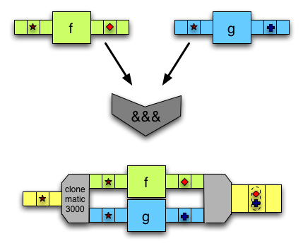
(&&&)takes one input, duplicates it and modifies each copy with a different arrow.


mean1 arrow from the tutorial. Rectangles are arrows, rounded rectangles are arrows made with arr, circles are other data flow split/merge points. Other combinators are left implicit. Corresponding code: (total &&& (const 1 ^>> total))
>>> arr (uncurry (/))It is worth mentioning that Control.Arrow defines returnA = arr id as a do-nothing arrow. One of the arrow laws says returnA must be equivalent to the id from the Category instance [6].
An ArrowChoice can be resolute
If Arrow makes multitasking possible, ArrowChoice forces a decision on what task to do.
class Arrow y => ArrowChoice y where
-- Minimal implementation: left
left :: y a b -> y (Either a c) (Either b c) -- maps over left choice
right :: y a b -> y (Either c a) (Either c b) -- maps over right choice
(+++) :: y a c -> y b d -> y (Either a b) (Either c d) -- left and right combined
(|||) :: y a c -> y b c -> y (Either a b) c -- (+++), then merge resultsEither provides a way to tag the values, so that different arrows can handle them depending on whether they are tagged with Left or Right. Note that these methods involving Either are entirely analogous to those involving pairs offered by Arrow.

getWord example of the tutorial. Blue indicates a Left tag and red indicates Right. Note that the if construct of proc notation sends True to Left and False to Right. Corresponding code:proc () -> do
firstTime <- oneShot -< ()
mPicked <- if firstTime
then do
picked <- pickWord rng -< ()
returnA -< Just picked
else returnA -< Nothing
accum' Nothing mplus -< mPickedAn ArrowApply is just boring
As the name suggests, ArrowApply makes it possible to apply arrows to values directly midway through an arrow computation. Ordinary Arrows do not allow that − we can just compose them on and on and on. Application only happens right at the end, once a run-arrow function of some sort is used to get a plain function from the arrow.
class Arrow y => ArrowApply y where
app :: y (y a b, a) b -- applies first component to second(For instance, app for functions is uncurry ($) = \(f, x) -> f x .)
app, however, comes at a steep price. Building an arrow as a value within an arrow computation and then eliminating it through application implies allowing the values within the computation to affect the context. That sounds a lot like what monadic binds do. It turns out that an ArrowApply is exactly equivalent to some Monad as long as the ArrowApply laws are followed. The ultimate consequence is that ArrowApply arrows cannot realise any of the interesting possibilities Arrow allows but Monad doesn't, such as having a partly static context.
The real flexibility with arrows comes with the ones that aren't monads, otherwise it's just a clunkier syntax.—Philippa Cowderoy
Arrow combinators crop up in unexpected places
Functions are the trivial example of arrows, and so all of the Control.Arrow functions shown above can be used with them. For that reason, it is quite common to see arrow combinators being used in code that otherwise has nothing to do with arrows. Here is a summary of what they do with plain functions, alongside with combinators in other modules that can be used in the same way (in case you prefer the alternative names, or just prefer using simple modules for simple tasks).
| Combinator | What it does (specialised to (->))
|
Alternatives |
|---|---|---|
(>>>) |
flip (.) |
|
first |
\f (x, y) -> (f x, y) |
first (Data.Bifunctor)
|
second |
\f (x, y) -> (x, f y) |
fmap; second (Data.Bifunctor)
|
(***) |
\f g (x, y) -> (f x, g y) |
bimap (Data.Bifunctor)
|
(&&&) |
\f g x -> (f x, g x) |
liftA2 (,) (Control.Applicative)
|
left |
Maps over Left case. |
first (Data.Bifunctor)
|
right |
Maps over Right case. |
fmap; second (Data.Bifunctor)
|
(+++) |
Maps over both cases. | bimap (Data.Bifunctor)
|
(|||) |
Eliminates Either. |
either (Data.Either)
|
app |
\(f, x) -> f x |
uncurry ($)
|
The Data.Bifunctor module provides the Bifunctor class, of which pairs and Either are instances. A Bifunctor is very much like a Functor, except that there are two independent ways of mapping functions over it, corresponding to the first and second methods [7].
| Exercises |
|---|
|
Using arrows
Avoiding leaks
Arrows were originally motivated by an efficient parser design found by Swierstra and Duponcheel[8]. In order to have a reference point for discussing the benefits of their design, let's begin with a very quick look at how monadic parsers work.
Here is a really bare-bones illustration of a monadic parser type:
newtype Parser s a = Parser { runParser :: [s] -> Maybe (a, [s]) }A Parser is a function that takes a stream of input (here, a list of type [s]), and, depending on what it finds in the input, returns either a result (of type [a]) and a stream (often, the input stream minus some of the input that is consumed by the parser), or Nothing. When we say a parser succeeded or failed, we refer to whether it produced a result. While real world parser types, such as ParsecT from Parsec [9], can be a lot more complex in order to provide various other features (notably, informative error messages upon failure), this simple Parser is good enough for our current purposes.
For instance, this is a parser for a single character in a string:
char :: Char -> Parser Char Char
char c = Parser $ \input -> case input of
[] -> Nothing
x : xs -> if x == c then Just (c, xs) else NothingIf the first character in the input string is c, char c succeeds, consuming the first character and giving c as a result; otherwise, it fails:
GHCi> runParser (char 'H') "Hello"
Just ('H',"ello")
GHCi> runParser (char 'G') "Hello"
NothingA second look at the Parser type shows it is essentially State [s] over Maybe. As such, it is not surprising we can make it an instance of Applicative, Monad, Alternative, and so forth (you might want to give it a try). That gives us a very flexible set of combinators for building more complex parsers out of simpler ones. Parsers can be run in sequence...
isHel :: Parser Char ()
isHel = char 'H' *> char 'e' *> char 'l' *> pure ()... have their results combined...
string :: String -> Parser Char String
string = traverse char... or be tried as alternatives to each other:
solfege :: Parser Char String
solfege = string "Do" <|> string "Re" <|> string "Mi"Through this last example, we can indicate which issue Swierstra and Duponcheel were trying to tackle. When solfege is run on the string "Fa", we can't detect the parser will fail until all of the three alternatives have failed. If we had more complex parsers in which one of the alternatives might fail only after attempting to consume a lot of the input stream, we would have to descend down the chain of parsers in the very same way. All of the input that can possibly be consumed by later parsers must be retained in memory in case one of them happens to be able to consume it. That can lead to much more space usage than you would naively expect − a situation often called a space leak.
Can it be done better?
Swierstra and Duponcheel (1996) noticed that, when dealing with some kinds of parsing tasks, a smarter parser could immediately fail upon seeing the very first character. For example, in the solfege parser above, the choice of first letter parsers was limited to letters 'D', 'R' and 'M', for "Do", "Re" and "Mi" respectively. This smarter parser would also be able to garbage collect input sooner because it could look ahead to see if any other parsers might be able to consume the input, and drop input that could not be consumed. This new parser is a lot like the monadic parsers with the major difference that it exports static information. It's like a monad, but it also tells you what it can parse.
There's one major problem. This doesn't fit into the Monad interface. Monadic composition works with (a -> m b) functions, and functions alone. There's no way to attach static information. You have only one choice, throw in some input, and see if it passes or fails.
Back when this issue first arose, the monadic interface was being touted as a completely general purpose tool in the functional programming community, so finding that there was some particularly useful code that just couldn't fit into that interface was something of a setback. This is where arrows come in. John Hughes's Generalising monads to arrows proposed the arrows abstraction as new, more flexible tool.
Static and dynamic parsers
Let us examine Swierstra and Duponcheel's parser in greater detail, from the perspective of arrows as presented by Hughes. The parser has two components: a fast, static parser which tells us if the input is worth trying to parse; and a slow, dynamic parser which does the actual parsing work.
import Control.Arrow
import qualified Control.Category as Cat
import Data.List (union)
data Parser s a b = P (StaticParser s) (DynamicParser s a b)
data StaticParser s = SP Bool [s]
newtype DynamicParser s a b = DP ((a, [s]) -> (b, [s]))The static parser consists of a flag, which tells us if the parser can accept the empty input, and a list of possible starting characters. For example, the static parser for a single character would be as follows:
spCharA :: Char -> StaticParser Char
spCharA c = SP False [c]It does not accept the empty string (False) and the list of possible starting characters consists only of c.
The dynamic parser needs a little more dissecting. What we see is a function that goes from (a, [s]) to (b, [s]). It is useful to think in terms of sequencing two parsers: each parser consumes the result of the previous parser (a), along with the remaining bits of input stream ([s]), it does something with a to produce its own result b, consumes a bit of string and returns that. So, as an example of this in action, consider a dynamic parser (Int, String) -> (Int, String), where the Int represents a count of the characters parsed so far. The table below shows what would happen if we sequence a few of them together and set them loose on the string "cake" :
| result | remaining | |
|---|---|---|
| before | 0 | cake |
| after first parser | 1 | ake |
| after second parser | 2 | ke |
| after third parser | 3 | e |
So the point here is that a dynamic parser has two jobs : it does something to the output of the previous parser (informally, a -> b), and it consumes a bit of the input string, (informally, [s] -> [s]), hence the type DP ((a,[s]) -> (b,[s])). Now, in the case of a dynamic parser for a single character (type (Char, String) -> (Char, String)), the first job is trivial. We ignore the output of the previous parser, return the character we have parsed and consume one character off the stream:
dpCharA :: Char -> DynamicParser Char a Char
dpCharA c = DP (\(_,_:xs) -> (c,xs))This might lead you to ask a few questions. For instance, what's the point of accepting the output of the previous parser if we're just going to ignore it? And shouldn't the dynamic parser be making sure that the current character off the stream matches the character to be parsed by testing x == c? The answer to the second question is no − and in fact, this is part of the point: the work is not necessary because the check would already have been performed by the static parser. Naturally, things are only so simple because we are testing just one character. If we were writing a parser for several characters in sequence we would need dynamic parsers that actually tested the second and further characters; and if we wanted to build an output string by chaining several parsers of characters then we would need the output of previous parsers.
Time to put both parsers together. Here is our S+D style parser for a single character:
charA :: Char -> Parser Char a Char
charA c = P (SP False [c]) (DP (\(_,_:xs) -> (c,xs)))In order to actually use the parser, we need a runParser function that runs the static tests and applies the dynamic parser to the input:
-- The Eq constraint on s is needed so that we can use elem.
runParser :: Eq s => Parser s a b -> a -> [s] -> Maybe (b, [s])
runParser (P (SP emp _) (DP p)) a []
| emp = Just (p (a, []))
| otherwise = Nothing
runParser (P (SP _ start) (DP p)) a input@(x:_)
| x `elem` start = Just (p (a, input))
| otherwise = NothingNote how runParser gives out a function with type [s] -> Maybe (b, [s]) function, which is essentially the same as the monadic parser we demonstrated earlier on. Now we can use charA much in the same way we used char back then. (The main difference is the () which we pass as a dummy argument. That makes sense here because charA doesn't actually use the initial value of type a. With other parsers, though, that need not be the case.)
GHCi> runParser (charA 'D') () "Do"
Just ('D',"o")
GHCi> runParser (charA 'D') () "Re"
NothingBringing the arrow combinators in
With the preliminary bit of exposition done, we are now going to implement the Arrow class for Parser s, and by doing so, give you a glimpse of what makes arrows useful. So let's get started:
instance Eq s => Arrow (Parser s) wherearr should convert an arbitrary function into a parsing arrow. In this case, we have to use "parse" in a very loose sense: the resulting arrow accepts the empty string, and only the empty string (its set of first characters is []). Its sole job is to take the output of the previous parsing arrow and do something with it. That being so, it does not consume any input.
arr f = P (SP True []) (DP (\(b,s) -> (f b,s)))Likewise, the first combinator is relatively straightforward. Given a parser, we want to produce a new parser that accepts a pair of inputs (b,d). The first component of the input b, is what we actually want to parse. The second part passes through untouched:
first (P sp (DP p)) = P sp (DP (\((b,d),s) ->
let (c, s') = p (b,s)
in ((c,d),s')))We also have to supply the Category instance. id is entirely obvious, as id = arr id must hold:
instance Eq s => Cat.Category (Parser s) where
id = P (SP True []) (DP (\(b,s) -> (b,s)))
-- Or simply: id = P (SP True []) (DP id)On the other hand, the implementation of (.) requires a little more thought. We want to take two parsers, and return a combined parser incorporating the static and dynamic parsers of both arguments:
-- The Eq s constraint is needed for using union here.
(P (SP empty1 start1) (DP p1)) .
(P (SP empty2 start2) (DP p2)) =
P (SP (empty1 && empty2)
(if not empty1 then start1 else start1 `union` start2))
(DP (p2.p1))Combining the dynamic parsers is easy enough; we just do function composition. Putting the static parsers together requires a little bit of thought. First of all, the combined parser can only accept the empty string if both parsers do. Fair enough, now how about the starting symbols? Well, the parsers are supposed to be in a sequence, so the starting symbols of the second parser shouldn't really matter. If life were simple, the starting symbols of the combined parser would only be start1. Alas, life is not simple, because parsers could very well accept the empty input. If the first parser accepts the empty input, then we have to account for this possibility by accepting the starting symbols from both the first and the second parsers
So what do arrows buy us?
If you look back at our Parser type and blank out the static parser section, you might notice that this looks a lot like the arrow instances for functions.
arr f = \(b, s) -> (f b, s)
first p = \((b, d), s) ->
let (c, s') = p (b, s)
in ((c, d), s'))
id = id
p2 . p1 = p2 . p1There's the odd s variable out for the ride, which makes the definitions look a little strange, but the outline of e.g. the simple first functions is there. Actually, what you see here is roughly the arrow instance for the State monad/Kleisli morphism (let f :: b -> c, p :: b -> State s c and (.) actually be (<=<) = flip (>=>)).
That's fine, but we could have easily done that with bind in classic monadic style, with first becoming just an odd helper function that could be easily written with a bit of pattern matching. But remember, our Parser type is not just the dynamic parser − it also contains the static parser.
arr f = SP True []
first sp = sp
(SP empty1 start1) >>> (SP empty2 start2) = (SP (empty1 && empty2)
(if not empty1 then start1 else start1 `union` start2))This is not at all a function, it's just pushing around some data types, and it cannot be expressed in a monadic way. But the Arrow interface can deal with just as well. And when we combine the two types, we get a two-for-one deal: the static parser data structure goes along for the ride along with the dynamic parser. The Arrow interface lets us transparently compose and manipulate the two parsers, static and dynamic, as a unit, which we can then run as a traditional, unified function.
Arrows in practice
Some examples of libraries using arrows:
- Opaleye (library documentation), a library for SQL generation.
- The Haskell XML Toolbox (project page and library documentation) uses arrows for processing XML. There is a Wiki page in the Haskell Wiki with a somewhat Gentle Introduction to HXT.
- Netwire (library documentation) is a library for functional reactive programming (FRP). FRP is a functional paradigm for handling events and time-varying values, with use cases including user interfaces, simulations and games. Netwire has an arrow interface as well as an applicative one.
- Yampa (Haskell Wiki page library documentation) is another arrow-based FRP library, and a predecessor to Netwire.
- Hughes' arrow-style parsers were first described in his 2000 paper, but a usable implementation wasn't available until May 2005, when Einar Karttunen released PArrows.
See also
Notes
- ↑ The paper that introduced arrows. It is freely accessible through its publisher.
- ↑ Those two concepts are usually known as static arrows and Kleisli arrows respectively. Since using the word "arrow" with two subtly different meanings would make this text horribly confusing, we opted for "morphism", which is a synonym for this alternative meaning.
- ↑ Incidentally, that is why they are called static: the effects are set in stone by the sequencing of computations; the generated values cannot affect them.
- ↑ For details, see Idioms are oblivious, arrows are meticulous, monads are promiscuous, by Sam Lindley, Philip Wadler and Jeremy Yallop.
- ↑ "Conveniently" is arguably too strong a word, though, given how confusing handling nested tuples can get. Ergo,
procnotation. - ↑
Arrowhas laws, and so do the other arrow classes we are discussing in these two chapters. We won't pause to pore over the laws here, but you can check them in the Control.Arrow documentation. - ↑
Data.Bifunctorwas only added to the core GHC libraries in version 7.10, so it might not be installed if you are using an older version. In that case, you can install thebifunctorspackage, which also includes several other bifunctor-related modules - ↑ Swierstra, Duponcheel. Deterministic, error correcting parser combinators. doi:10.1007/3-540-61628-4_7
- ↑ Parsec is a popular and powerful parsing library. See the parsec documentation on Hackage for more information.
Acknowledgements
This module uses text from An Introduction to Arrows by Shae Erisson, originally written for The Monad.Reader 4
Continuation passing style (CPS)
Continuation Passing Style (CPS for short) is a style of programming in which functions do not return values; rather, they pass control onto a continuation, which specifies what happens next. In this chapter, we are going to consider how that plays out in Haskell and, in particular, how CPS can be expressed with a monad.
What are continuations?
To dispel puzzlement, we will have a second look at an example from way back in the book, when we introduced the ($) operator:
> map ($ 2) [(2*), (4*), (8*)] [4,8,16]
There is nothing out of ordinary about the expression above, except that it is a little quaint to write that instead of map (*2) [2, 4, 8]. The ($) section makes the code appear backwards, as if we are applying a value to the functions rather than the other way around. And now, the catch: such an innocent-looking reversal is at heart of continuation passing style!
From a CPS perspective, ($ 2) is a suspended computation: a function with general type (a -> r) -> r which, given another function as argument, produces a final result. The a -> r argument is the continuation; it specifies how the computation will be brought to a conclusion. In the example, the functions in the list are supplied as continuations via map, producing three distinct results. Note that suspended computations are largely interchangeable with plain values: flip ($) [1] converts any value into a suspended computation, and passing id as its continuation gives back the original value.
What are they good for?
There is more to continuations than just a parlour trick to impress Haskell newbies. They make it possible to explicitly manipulate, and dramatically alter, the control flow of a program. For instance, returning early from a procedure can be implemented with continuations. Exceptions and failure can also be handled with continuations - pass in a continuation for success, another continuation for fail, and invoke the appropriate continuation. Other possibilities include "suspending" a computation and returning to it at another time, and implementing simple forms of concurrency (notably, one Haskell implementation, Hugs, uses continuations to implement cooperative concurrency).
In Haskell, continuations can be used in a similar fashion, for implementing interesting control flow in monads. Note that there usually are alternative techniques for such use cases, especially in tandem with laziness. In some circumstances, CPS can be used to improve performance by eliminating certain construction-pattern matching sequences (i.e. a function returns a complex structure which the caller will at some point deconstruct), though a sufficiently smart compiler should be able to do the elimination [2].
Passing continuations
An elementary way to take advantage of continuations is to modify our functions so that they return suspended computations rather than ordinary values. We will illustrate how that is done with two simple examples.
pythagoras
Example: A simple module, no continuations
-- We assume some primitives add and square for the example:
add :: Int -> Int -> Int
add x y = x + y
square :: Int -> Int
square x = x * x
pythagoras :: Int -> Int -> Int
pythagoras x y = add (square x) (square y)Modified to return a suspended computation, pythagoras looks like this:
Example: A simple module, using continuations
-- We assume CPS versions of the add and square primitives,
-- (note: the actual definitions of add_cps and square_cps are not
-- in CPS form, they just have the correct type)
add_cps :: Int -> Int -> ((Int -> r) -> r)
add_cps x y = \k -> k (add x y)
square_cps :: Int -> ((Int -> r) -> r)
square_cps x = \k -> k (square x)
pythagoras_cps :: Int -> Int -> ((Int -> r) -> r)
pythagoras_cps x y = \k ->
square_cps x $ \x_squared ->
square_cps y $ \y_squared ->
add_cps x_squared y_squared $ kHow the pythagoras_cps example works:
- square x and throw the result into the (\x_squared -> ...) continuation
- square y and throw the result into the (\y_squared -> ...) continuation
- add x_squared and y_squared and throw the result into the top level/program continuation
k.
We can try it out in GHCi by passing print as the program continuation:
*Main> pythagoras_cps 3 4 print 25
If we look at the type of pythagoras_cps without the optional parentheses around (Int -> r) -> r and compare it with the original type of pythagoras, we note that the continuation was in effect added as an extra argument, thus justifying the "continuation passing style" moniker.
thrice
Example: A simple higher order function, no continuations
thrice :: (a -> a) -> a -> a
thrice f x = f (f (f x))*Main> thrice tail "foobar" "bar"
A higher order function such as thrice, when converted to CPS, takes as arguments functions in CPS form as well. Therefore, f :: a -> a will become f_cps :: a -> ((a -> r) -> r), and the final type will be thrice_cps :: (a -> ((a -> r) -> r)) -> a -> ((a -> r) -> r). The rest of the definition follows quite naturally from the types - we replace f by the CPS version, passing along the continuation at hand.
Example: A simple higher order function, with continuations
thrice_cps :: (a -> ((a -> r) -> r)) -> a -> ((a -> r) -> r)
thrice_cps f_cps x = \k ->
f_cps x $ \fx ->
f_cps fx $ \ffx ->
f_cps ffx $ kThe Cont monad
Having continuation-passing functions, the next step is providing a neat way of composing them, preferably one which does not require the long chains of nested lambdas we have seen just above. A good start would be a combinator for applying a CPS function to a suspended computation. A possible type for it would be:
chainCPS :: ((a -> r) -> r) -> (a -> ((b -> r) -> r)) -> ((b -> r) -> r)(You may want to try implementing it before reading on. Hint: start by stating that the result is a function which takes a b -> r continuation; then, let the types guide you.)
And here is the implementation:
chainCPS s f = \k -> s $ \x -> f x $ kWe supply the original suspended computation s with a continuation which makes a new suspended computation (produced by f) and passes the final continuation k to it. Unsurprisingly, it mirrors closely the nested lambda pattern of the previous examples.
Doesn't the type of chainCPS look familiar? If we replace (a -> r) -> r with (Monad m) => m a and (b -> r) -> r with (Monad m) => m b we get the (>>=) signature. Furthermore, our old friend flip ($) plays a return-like role, in that it makes a suspended computation out of a value in a trivial way. Lo and behold, we have a monad! All we need now [3] is a Cont r a type to wrap suspended computations, with the usual wrapper and unwrapper functions.
cont :: ((a -> r) -> r) -> Cont r a
runCont :: Cont r a -> (a -> r) -> rThe monad instance for Cont follows directly from our presentation, the only difference being the wrapping and unwrapping cruft:
instance Monad (Cont r) where
return x = cont ($ x)
s >>= f = cont $ \c -> runCont s $ \x -> runCont (f x) cThe end result is that the monad instance makes the continuation passing (and thus the lambda chains) implicit. The monadic bind applies a CPS function to a suspended computation, and runCont is used to provide the final continuation. For a simple example, the Pythagoras example becomes:
Example: The pythagoras example, using the Cont monad
-- Using the Cont monad from the transformers package.
import Control.Monad.Trans.Cont
add_cont :: Int -> Int -> Cont r Int
add_cont x y = return (add x y)
square_cont :: Int -> Cont r Int
square_cont x = return (square x)
pythagoras_cont :: Int -> Int -> Cont r Int
pythagoras_cont x y = do
x_squared <- square_cont x
y_squared <- square_cont y
add_cont x_squared y_squaredcallCC
While it is always pleasant to see a monad coming forth naturally, a hint of disappointment might linger at this point. One of the promises of CPS was precise control flow manipulation through continuations. And yet, after converting our functions to CPS we promptly hid the continuations behind a monad. To rectify that, we shall introduce callCC, a function which gives us back explicit control of continuations - but only where we want it.
callCC is a very peculiar function; one that is best introduced with examples. Let us start with a trivial one:
Example: square using callCC
-- Without callCC
square :: Int -> Cont r Int
square n = return (n ^ 2)
-- With callCC
squareCCC :: Int -> Cont r Int
squareCCC n = callCC $ \k -> k (n ^ 2)The argument passed to callCC is a function, whose result is a suspended computation (general type Cont r a) which we will refer to as "the callCC computation". In principle, the callCC computation is what the whole callCC expression evaluates to. The caveat, and what makes callCC so special, is due to k, the argument to the argument. It is a function which acts as an eject button: calling it anywhere will lead to the value passed to it being made into a suspended computation, which then is inserted into control flow at the point of the callCC invocation. That happens unconditionally; in particular, whatever follows a k invocation in the callCC computation is summarily discarded. From another perspective, k captures the rest of the computation following the callCC; calling it throws a value into the continuation at that particular point ("callCC" stands for "call with current continuation"). While in this simple example the effect is merely that of a plain return, callCC opens up a number of possibilities, which we are now going to explore.
Deciding when to use k
callCC gives us extra power over what is thrown into a continuation, and when that is done. The following example begins to show how we can use this extra power.
Example: Our first proper callCC function
foo :: Int -> Cont r String
foo x = callCC $ \k -> do
let y = x ^ 2 + 3
when (y > 20) $ k "over twenty"
return (show $ y - 4)foo is a slightly pathological function that computes the square of its input and adds three; if the result of this computation is greater than 20, then we return from the callCC computation (and, in this case, from the whole function) immediately, throwing the string "over twenty" into the continuation that will be passed to foo. If not, then we subtract four from our previous computation, show it, and throw it into the continuation. Remarkably, k here is used just like the 'return' statement from an imperative language, that immediately exits the function. And yet, this being Haskell, k is just an ordinary first-class function, so you can pass it to other functions like when, store it in a Reader, etc.
Naturally, you can embed calls to callCC within do-blocks:
Example: More developed callCC example involving a do-block
bar :: Char -> String -> Cont r Int
bar c s = do
msg <- callCC $ \k -> do
let s0 = c : s
when (s0 == "hello") $ k "They say hello."
let s1 = show s0
return ("They appear to be saying " ++ s1)
return (length msg)When you call k with a value, the entire callCC call takes that value. In effect, that makes k a lot like an 'goto' statement in other languages: when we call k in our example, it pops the execution out to where you first called callCC, the msg <- callCC $ ... line. No more of the argument to callCC (the inner do-block) is executed. Hence the following example contains a useless line:
Example: Popping out a function, introducing a useless line
quux :: Cont r Int
quux = callCC $ \k -> do
let n = 5
k n
return 25quux will return 5, and not 25, because we pop out of quux before getting to the return 25 line.
Behind the scenes
We have deliberately broken a trend here: normally when we introduce a function we give its type straight away, but in this case we chose not to. The reason is simple: the type is pretty complex, and it does not immediately give insight into what the function does, or how it works. After the initial presentation of callCC, however, we are in a better position to tackle it. Take a deep breath...
callCC :: ((a -> Cont r b) -> Cont r a) -> Cont r aWe can make sense of that based on what we already know about callCC. The overall result type and the result type of the argument have to be the same (i.e. Cont r a), as in the absence of an invocation of k the corresponding result values are one and the same. Now, what about the type of k? As mentioned above, k's argument is made into a suspended computation inserted at the point of the callCC invocation; therefore, if the latter has type Cont r a k's argument must have type a. As for k's result type, interestingly enough it doesn't matter as long as it is wrapped in the same Cont r monad; in other words, the b stands for an arbitrary type. That happens because the suspended computation made out of the a argument will receive whatever continuation follows the callCC, and so the continuation taken by k's result is irrelevant.
Note
The arbitrariness of k's result type explains why the following variant of the useless line example leads to a type error:
quux :: Cont r Int
quux = callCC $ \k -> do
let n = 5
when True $ k n
k 25k's result type could be anything of form Cont r b; however, the when constrains it to Cont r (), and so the closing k 25 does not match the result type of quux. The solution is very simple: replace the final k by a plain old return.
To conclude this section, here is the implementation of callCC. Can you identify k in it?
callCC f = cont $ \h -> runCont (f (\a -> cont $ \_ -> h a)) hThough the code is far from obvious, an amazing fact is that the implementations of callCC, return and (>>=) for Cont can be produced automatically from their type signatures - Lennart Augustsson's Djinn [6] is a program that will do this for you. See Phil Gossett's Google tech talk: [7] for background on the theory behind Djinn; and Dan Piponi's article: [8] which uses Djinn in deriving continuation passing style.
Example: a complicated control structure
We will now look at some more realistic examples of control flow manipulation. The first one, presented below, was originally taken from "The Continuation monad" section of the All about monads tutorial, used with permission.
Example: Using Cont for a complicated control structure
{- We use the continuation monad to perform "escapes" from code blocks.
This function implements a complicated control structure to process
numbers:
Input (n) Output List Shown
========= ====== ==========
0-9 n none
10-199 number of digits in (n/2) digits of (n/2)
200-19999 n digits of (n/2)
20000-1999999 (n/2) backwards none
>= 2000000 sum of digits of (n/2) digits of (n/2)
-}
fun :: Int -> String
fun n = (`runCont` id) $ do
str <- callCC $ \exit1 -> do -- define "exit1"
when (n < 10) (exit1 (show n))
let ns = map digitToInt (show (n `div` 2))
n' <- callCC $ \exit2 -> do -- define "exit2"
when ((length ns) < 3) (exit2 (length ns))
when ((length ns) < 5) (exit2 n)
when ((length ns) < 7) $ do
let ns' = map intToDigit (reverse ns)
exit1 (dropWhile (=='0') ns') --escape 2 levels
return $ sum ns
return $ "(ns = " ++ (show ns) ++ ") " ++ (show n')
return $ "Answer: " ++ strfun is a function that takes an integer n. The implementation uses Cont and callCC to set up a control structure using Cont and callCC that does different things based on the range that n falls in, as stated by the comment at the top. Let us dissect it:
- Firstly, the
(`runCont` id)at the top just means that we run theContblock that follows with a final continuation ofid(or, in other words, we extract the value from the suspended computation unchanged). That is necessary as the result type offundoesn't mentionCont. - We bind
strto the result of the followingcallCCdo-block:- If
nis less than 10, we exit straight away, just showingn. - If not, we proceed. We construct a list,
ns, of digits ofn `div` 2. n'(anInt) gets bound to the result of the following innercallCCdo-block.- If
length ns < 3, i.e., ifn `div` 2has less than 3 digits, we pop out of this inner do-block with the number of digits as the result. - If
n `div` 2has less than 5 digits, we pop out of the inner do-block returning the originaln. - If
n `div` 2has less than 7 digits, we pop out of both the inner and outer do-blocks, with the result of the digits ofn `div` 2in reverse order (aString). - Otherwise, we end the inner do-block, returning the sum of the digits of
n `div` 2.
- If
- We end this do-block, returning the String
"(ns = X) Y", where X isns, the digits ofn `div` 2, and Y is the result from the inner do-block,n'.
- If
- Finally, we return out of the entire function, with our result being the string "Answer: Z", where Z is the string we got from the
callCCdo-block.
Example: exceptions
One use of continuations is to model exceptions. To do this, we hold on to two continuations: one that takes us out to the handler in case of an exception, and one that takes us to the post-handler code in case of a success. Here's a simple function that takes two numbers and does integer division on them, failing when the denominator is zero.
Example: An exception-throwing div
divExcpt :: Int -> Int -> (String -> Cont r Int) -> Cont r Int
divExcpt x y handler = callCC $ \ok -> do
err <- callCC $ \notOk -> do
when (y == 0) $ notOk "Denominator 0"
ok $ x `div` y
handler err
{- For example,
runCont (divExcpt 10 2 error) id --> 5
runCont (divExcpt 10 0 error) id --> *** Exception: Denominator 0
-}How does it work? We use two nested calls to callCC. The first labels a continuation that will be used when there's no problem. The second labels a continuation that will be used when we wish to throw an exception. If the denominator isn't 0, x `div` y is thrown into the ok continuation, so the execution pops right back out to the top level of divExcpt. If, however, we were passed a zero denominator, we throw an error message into the notOk continuation, which pops us out to the inner do-block, and that string gets assigned to err and given to handler.
A more general approach to handling exceptions can be seen with the following function. Pass a computation as the first parameter (more precisely, a function which takes an error-throwing function and results in the computation) and an error handler as the second parameter. This example takes advantage of the generic MonadCont class [4] which covers both Cont and the corresponding ContT transformer by default, as well as any other continuation monad which instantiates it.
Example: General try using continuations.
import Control.Monad.Cont
tryCont :: MonadCont m => ((err -> m a) -> m a) -> (err -> m a) -> m a
tryCont c h = callCC $ \ok -> do
err <- callCC $ \notOk -> do
x <- c notOk
ok x
h errAnd here is our try in action:
Example: Using try
data SqrtException = LessThanZero deriving (Show, Eq)
sqrtIO :: (SqrtException -> ContT r IO ()) -> ContT r IO ()
sqrtIO throw = do
ln <- lift (putStr "Enter a number to sqrt: " >> readLn)
when (ln < 0) (throw LessThanZero)
lift $ print (sqrt ln)
main = runContT (tryCont sqrtIO (lift . print)) returnIn this example, error throwing means escaping from an enclosing callCC. The throw in sqrtIO jumps out of tryCont's inner callCC.
Example: coroutines
In this section we make a CoroutineT monad that provides a monad with fork, which enqueues a new suspended coroutine, and yield, that suspends the current thread.
{-# LANGUAGE GeneralizedNewtypeDeriving #-}
-- We use GeneralizedNewtypeDeriving to avoid boilerplate. As of GHC 7.8, it is safe.
import Control.Applicative
import Control.Monad.Cont
import Control.Monad.State
-- The CoroutineT monad is just ContT stacked with a StateT containing the suspended coroutines.
newtype CoroutineT r m a = CoroutineT {runCoroutineT' :: ContT r (StateT [CoroutineT r m ()] m) a}
deriving (Functor,Applicative,Monad,MonadCont,MonadIO)
-- Used to manipulate the coroutine queue.
getCCs :: Monad m => CoroutineT r m [CoroutineT r m ()]
getCCs = CoroutineT $ lift get
putCCs :: Monad m => [CoroutineT r m ()] -> CoroutineT r m ()
putCCs = CoroutineT . lift . put
-- Pop and push coroutines to the queue.
dequeue :: Monad m => CoroutineT r m ()
dequeue = do
current_ccs <- getCCs
case current_ccs of
[] -> return ()
(p:ps) -> do
putCCs ps
p
queue :: Monad m => CoroutineT r m () -> CoroutineT r m ()
queue p = do
ccs <- getCCs
putCCs (ccs++[p])
-- The interface.
yield :: Monad m => CoroutineT r m ()
yield = callCC $ \k -> do
queue (k ())
dequeue
fork :: Monad m => CoroutineT r m () -> CoroutineT r m ()
fork p = callCC $ \k -> do
queue (k ())
p
dequeue
-- Exhaust passes control to suspended coroutines repeatedly until there isn't any left.
exhaust :: Monad m => CoroutineT r m ()
exhaust = do
exhausted <- null <$> getCCs
if not exhausted
then yield >> exhaust
else return ()
-- Runs the coroutines in the base monad.
runCoroutineT :: Monad m => CoroutineT r m r -> m r
runCoroutineT = flip evalStateT [] . flip runContT return . runCoroutineT' . (<* exhaust)Some example usage:
printOne n = do
liftIO (print n)
yield
example = runCoroutineT $ do
fork $ replicateM_ 3 (printOne 3)
fork $ replicateM_ 4 (printOne 4)
replicateM_ 2 (printOne 2)Outputting:
3 4 3 2 4 3 2 4 4
Example: Implementing pattern matching
An interesting usage of CPS functions is to implement our own pattern matching. We will illustrate how this can be done by some examples.
Example: Built-in pattern matching
check :: Bool -> String
check b = case b of
True -> "It's True"
False -> "It's False"Now we have learnt CPS, we can refactor the code like this.
Example: Pattern matching in CPS
type BoolCPS r = r -> r -> r
true :: BoolCPS r
true x _ = x
false :: BoolCPS r
false _ x = x
check :: BoolCPS String -> String
check b = b "It's True" "It's False"*Main> check true "It's True" *Main> check false "It's False"
What happens here is that, instead of plain values, we represent True and False by functions that would choose either the first or second argument they are passed. Since true and false behave differently, we can achieve the same effect as pattern matching. Furthermore, True, False and true, false can be converted back and forth by \b -> b True False and \b -> if b then true else false.
We should see how this is related to CPS in this more complicated example.
Example: More complicated pattern matching and its CPS equivalence
data Foobar = Zero | One Int | Two Int Int
type FoobarCPS r = r -> (Int -> r) -> (Int -> Int -> r) -> r
zero :: FoobarCPS r
zero x _ _ = x
one :: Int -> FoobarCPS r
one x _ f _ = f x
two :: Int -> Int -> FoobarCPS r
two x y _ _ f = f x y
fun :: Foobar -> Int
fun x = case x of
Zero -> 0
One a -> a + 1
Two a b -> a + b + 2
funCPS :: FoobarCPS Int -> Int
funCPS x = x 0 (+1) (\a b -> a + b + 2)*Main> fun Zero 0 *Main> fun $ One 3 4 *Main> fun $ Two 3 4 9 *Main> funCPS zero 0 *Main> funCPS $ one 3 4 *Main> funCPS $ two 3 4 9
Similar to former example, we represent values by functions. These function-values pick the corresponding (i.e. match) continuations they are passed to and pass to the latter the values stored in the former. An interesting thing is that this process involves in no comparison. As we know, pattern matching can work on types that are not instances of Eq: the function-values "know" what their patterns are and would automatically pick the right continuations. If this is done from outside, say, by an pattern_match :: [(pattern, result)] -> value -> result function, it would have to inspect and compare the patterns and the values to see if they match -- and thus would need Eq instances.
Notes
- ↑ That is,
\x -> ($ x), fully spelled out as\x -> \k -> k x - ↑ attoparsec is an example of performance-driven usage of CPS.
- ↑ Beyond verifying that the monad laws hold, which is left as an exercise to the reader.
- ↑ Found in the
mtlpackage, module Control.Monad.Cont.
Zippers
Theseus and the Zipper
The Labyrinth
"Theseus, we have to do something" said Homer, chief marketing officer of Ancient Geeks Inc.. Theseus put the Minotaur action figure™ back onto the shelf and nodded. "Today's children are no longer interested in the ancient myths, they prefer modern heroes like Spiderman or Sponge Bob." Heroes. Theseus knew well how much he had been a hero in the labyrinth back then on Crete[1]. But those "modern heroes" did not even try to appear realistic. What made them so successful? Anyway, if the pending sales problems could not be resolved, the shareholders would certainly arrange a passage over the Styx for Ancient Geeks Inc.
"Heureka! Theseus, I have an idea: we implement your story with the Minotaur as a computer game! What do you say?" Homer was right. There had been several books, epic (and chart breaking) songs, a mandatory movie trilogy and uncountable Theseus & the Minotaur™ gimmicks, but a computer game was missing. "Perfect, then. Now, Theseus, your task is to implement the game".
A true hero, Theseus chose Haskell as the language to implement the company's redeeming product in. Of course, exploring the labyrinth of the Minotaur was to become one of the game's highlights. He pondered: "We have a two-dimensional labyrinth whose corridors can point in many directions. Of course, we can abstract from the detailed lengths and angles: for the purpose of finding the way out, we only need to know how the path forks. To keep things easy, we model the labyrinth as a tree. This way, the two branches of a fork cannot join again when walking deeper and the player cannot go round in circles. But I think there is enough opportunity to get lost; and this way, if the player is patient enough, they can explore the entire labyrinth with the left-hand rule."
data Node a = DeadEnd a
| Passage a (Node a)
| Fork a (Node a) (Node a)

Theseus made the nodes of the labyrinth carry an extra parameter of type a. Later on, it may hold game relevant information like the coordinates of the spot a node designates, the ambience around it, a list of game items that lie on the floor, or a list of monsters wandering in that section of the labyrinth. We assume that two helper functions
get :: Node a -> a put :: a -> Node a -> Node a
retrieve and change the value of type a stored in the first argument of every constructor of Node a.
| Exercises |
|---|
|
"Mh, how to represent the player's current position in the labyrinth? The player can explore deeper by choosing left or right branches, like in"
turnRight :: Node a -> Maybe (Node a) turnRight (Fork _ l r) = Just r turnRight _ = Nothing
"But replacing the current top of the labyrinth with the corresponding sub-labyrinth this way is not an option, because the player cannot go back then." He pondered. "Ah, we can apply Ariadne's trick with the thread for going back. We simply represent the player's position by the list of branches their thread takes, the labyrinth always remains the same."
data Branch = KeepStraightOn
| TurnLeft
| TurnRight
type Thread = [Branch]

"For example, a thread [TurnRight,KeepStraightOn] means that the player took the right branch at the entrance and then went straight down a Passage to reach its current position. With the thread, the player can now explore the labyrinth by extending or shortening it. For instance, the function turnRight extends the thread by appending the TurnRight to it."
turnRight :: Thread -> Thread turnRight t = t ++ [TurnRight]
"To access the extra data, i.e. the game relevant items and such, we simply follow the thread into the labyrinth."
retrieve :: Thread -> Node a -> a retrieve [] n = get n retrieve (KeepStraightOn:bs) (Passage _ n) = retrieve bs n retrieve (TurnLeft :bs) (Fork _ l r) = retrieve bs l retrieve (TurnRight :bs) (Fork _ l r) = retrieve bs r
| Exercises |
|---|
Write a function update that applies a function of type a -> a to the extra data at the player's position. |
Theseus' satisfaction over this solution did not last long. "Unfortunately, if we want to extend the path or go back a step, we have to change the last element of the list. We could store the list in reverse, but even then, we have to follow the thread again and again to access the data in the labyrinth at the player's position. Both actions take time proportional to the length of the thread and for large labyrinths, this will be too long. Isn't there another way?"
Ariadne's Zipper
While Theseus was a skillful warrior, he did not train much in the art of programming and could not find a satisfying solution. After intense but fruitless cogitation, he decided to call his former love Ariadne to ask her for advice. After all, it was she who had the idea with the thread.
"Ariadne Consulting. What can I do for you?"
Our hero immediately recognized the voice.
"Hello Ariadne, it's Theseus."
An uneasy silence paused the conversation. Theseus remembered well that he had abandoned her on the island of Naxos and knew that she would not appreciate his call. But Ancient Geeks Inc. was on the road to Hades and he had no choice.
"Uhm, darling, ... how are you?"
Ariadne retorted an icy response, "Mr. Theseus, the times of darling are long over. What do you want?"
"Well, I uhm ... I need some help with a programming problem. I'm programming a new Theseus & the Minotaur™ computer game."
She jeered, "Yet another artifact to glorify your 'heroic being'? And you want me of all people to help you?"
"Ariadne, please, I beg of you, Ancient Geeks Inc. is on the brink of insolvency. The game is our last hope!"
After a pause, she came to a decision.
"Fine, I will help you. But only if you transfer a substantial part of Ancient Geeks Inc. to me. Let's say thirty percent."
Theseus turned pale. But what could he do? The situation was desperate enough, so he agreed but only after negotiating Ariadne's share to a tenth.
After Theseus told Ariadne of the labyrinth representation he had in mind, she could immediately give advice,
"You need a zipper."
"Huh? What does the problem have to do with my fly?"
"Nothing, it's a data structure first published by Gérard Huet[2]."
"Ah."
"More precisely, it's a purely functional way to augment tree-like data structures like lists or binary trees with a single focus or finger that points to a subtree inside the data structure and allows constant time updates and lookups at the spot it points to[3]. In our case, we want a focus on the player's position."
"I know for myself that I want fast updates, but how do I code it?"
"Don't get impatient, you cannot solve problems by coding, you can only solve them by thinking. The only place where we can get constant time updates in a purely functional data structure is the topmost node[4][5]. So, the focus necessarily has to be at the top. Currently, the topmost node in your labyrinth is always the entrance, but your previous idea of replacing the labyrinth by one of its sub-labyrinths ensures that the player's position is at the topmost node."
"But then, the problem is how to go back, because all those sub-labyrinths get lost that the player did not choose to branch into."
"Well, you can use my thread in order not to lose the sub-labyrinths."
Ariadne savored Theseus' puzzlement but quickly continued before he could complain that he already used Ariadne's thread,
"The key is to glue the lost sub-labyrinths to the thread so that they actually don't get lost at all. The intention is that the thread and the current sub-labyrinth complement one another to the whole labyrinth. With 'current' sub-labyrinth, I mean the one that the player stands on top of. The zipper simply consists of the thread and the current sub-labyrinth."
type Zipper a = (Thread a, Node a)

Theseus didn't say anything.
"You can also view the thread as a context in which the current sub-labyrinth resides. Now, let's find out how to define Thread a. By the way, Thread has to take the extra parameter a because it now stores sub-labyrinths. The thread is still a simple list of branches, but the branches are different from before."
data Branch a = KeepStraightOn a
| TurnLeft a (Node a)
| TurnRight a (Node a)
type Thread a = [Branch a]
"Most importantly, TurnLeft and TurnRight have a sub-labyrinth glued to them. When the player chooses say to turn right, we extend the thread with a TurnRight and now attach the untaken left branch to it, so that it doesn't get lost."
Theseus interrupts, "Wait, how would I implement this behavior as a function turnRight? And what about the first argument of type a for TurnRight? Ah, I see. We not only need to glue the branch that would get lost, but also the extra data of the Fork because it would otherwise get lost as well. So, we can generate a new branch by a preliminary"
branchRight (Fork x l r) = TurnRight x l
"Now, we have to somehow extend the existing thread with it."
"Indeed. The second point about the thread is that it is stored backwards. To extend it, you put a new branch in front of the list. To go back, you delete the topmost element."
"Aha, this makes extending and going back take only constant time, not time proportional to the length as in my previous version. So the final version of turnRight is"
turnRight :: Zipper a -> Maybe (Zipper a) turnRight (t, Fork x l r) = Just (TurnRight x l : t, r) turnRight _ = Nothing

"That was not too difficult. So let's continue with keepStraightOn for going down a passage. This is even easier than choosing a branch as we only need to keep the extra data:"
keepStraightOn :: Zipper a -> Maybe (Zipper a) keepStraightOn (t, Passage x n) = Just (KeepStraightOn x : t, n) keepStraightOn _ = Nothing

| Exercises |
|---|
Write the function turnLeft. |
Pleased, he continued, "But the interesting part is to go back, of course. Let's see..."
back :: Zipper a -> Maybe (Zipper a) back ([] , _) = Nothing back (KeepStraightOn x : t , n) = Just (t, Passage x n) back (TurnLeft x r : t , l) = Just (t, Fork x l r) back (TurnRight x l : t , r) = Just (t, Fork x l r)
"If the thread is empty, we're already at the entrance of the labyrinth and cannot go back. In all other cases, we have to wind up the thread. And thanks to the attachments to the thread, we can actually reconstruct the sub-labyrinth we came from."
Ariadne remarked, "Note that a partial test for correctness is to check that each bound variable like x, l and r on the left hand side appears exactly once at the right hands side as well. So, when walking up and down a zipper, we only redistribute data between the thread and the current sub-labyrinth."
| Exercises |
|---|
|
Heureka! That was the solution Theseus sought and Ancient Geeks Inc. should prevail, even if partially sold to Ariadne Consulting. But one question remained:
"Why is it called zipper?"
"Well, I would have called it 'Ariadne's pearl necklace'. But most likely, it's called zipper because the thread is in analogy to the open part and the sub-labyrinth is like the closed part of a zipper. Moving around in the data structure is analogous to zipping or unzipping the zipper."
"'Ariadne's pearl necklace'," he articulated disdainfully. "As if your thread was any help back then on Crete."
"As if the idea with the thread were yours," she replied.
"Bah, I need no thread," he defied the fact that he actually did need the thread to program the game.
Much to his surprise, she agreed, "Well, indeed you don't need a thread. Another view is to literally grab the tree at the focus with your finger and lift it up in the air. The focus will be at the top and all other branches of the tree hang down. You only have to assign the resulting tree a suitable algebraic data type, most likely that of the zipper."

"Ah." He didn't need Ariadne's thread but he needed Ariadne to tell him? That was too much.
"Thank you, Ariadne, good bye."
She did not hide her smirk as he could not see it anyway through the phone.
| Exercises |
|---|
| Take a list, fix one element in the middle with your finger and lift the list into the air. What type can you give to the resulting tree? |
Half a year later, Theseus stopped in front of a shop window, defying the cold rain that tried to creep under his buttoned up anorak. Blinking letters announced
- find your way through the labyrinth of threads -
the great computer game by Ancient Geeks Inc.
He cursed the day when he called Ariadne and sold her a part of the company. Was it she who contrived the unfriendly takeover by WineOS Corp., led by Ariadne's husband Dionysus? Theseus watched the raindrops finding their way down the glass window. After the production line was changed, nobody would produce Theseus and the Minotaur™ merchandise anymore. He sighed. His time, the time of heroes, was over. Now came the super-heroes.
Differentiation of data types
The previous section has presented the zipper, a way to augment a tree-like data structure Node a with a finger that can focus on the different subtrees. While we constructed a zipper for a particular data structure Node a, the construction can be easily adapted to different tree data structures by hand.
| Exercises |
|---|
|
Start with a ternary tree data Tree a = Leaf a | Node (Tree a) (Tree a) (Tree a)and derive the corresponding Thread a and Zipper a. |
Mechanical Differentiation
But there is also an entirely mechanical way to derive the zipper of any (suitably regular) data type. Surprisingly, 'derive' is to be taken literally, for the zipper can be obtained by the derivative of the data type, a discovery first described by Conor McBride[6]. The subsequent section is going to explicate this truly wonderful mathematical gem.
For a systematic construction, we need to calculate with types. The basics of structural calculations with types are outlined in a separate chapter Generic Programming and we will heavily rely on this material.
Let's look at some examples to see what their zippers have in common and how they hint differentiation. The type of binary tree is the fixed point of the recursive equation

When walking down the tree, we iteratively choose to enter the left or the right subtree and then glue the not-entered subtree to Ariadne's thread. Thus, the branches of our thread have the type

Similarly, the thread for a ternary tree

has branches of type

because at every step, we can choose between three subtrees and have to store the two subtrees we don't enter. Isn't this strikingly similar to the derivatives and ?


The key to the mystery is the notion of the one-hole context of a data structure. Imagine a data structure parameterised over a type , like the type of trees . If we were to remove one of the items of this type from the structure and somehow mark the now empty position, we obtain a structure with a marked hole. The result is called "one-hole context" and inserting an item of type into the hole gives back a completely filled . The hole acts as a distinguished position, a focus. The figures illustrate this.


 |
 |
Of course, we are interested in the type to give to a one-hole context, i.e. how to represent it in Haskell. The problem is how to efficiently mark the focus. But as we will see, finding a representation for one-hole contexts by induction on the structure of the type we want to take the one-hole context of automatically leads to an efficient data type[7]. So, given a data structure with a functor and an argument type , we want to calculate the type of one-hole contexts from the structure of . As our choice of notation already reveals, the rules for constructing one-hole contexts of sums, products and compositions are exactly Leibniz' rules for differentiation.


| One-hole context | Illustration | |
|---|---|---|
| There is no in , so the type of its one-hole contexts must be empty. | ||
| There is only one position for items in . Removing one leaves no in the result. And as there is only one position we can remove it from, there is exactly one one-hole context for . Thus, the type of one-hole contexts is the singleton type. | ||
| As an element of type is either of type or of type , a one-hole context is also either or . | ||
 The hole in a one-hole context of a pair is either in the first or in the second component. | ||
 Chain rule. The hole in a composition arises by making a hole in the enclosing structure and fitting the enclosed structure in. | ||


Of course, the function plug that fills a hole has the type .

So far, the syntax denotes the differentiation of functors, i.e. of a kind of type functions with one argument. But there is also a handy expression oriented notation slightly more suitable for calculation. The subscript indicates the variable with respect to which we want to differentiate. In general, we have


An example is

Of course, is just point-wise whereas is point-free style.
| Exercises |
|---|
|


Zippers via Differentiation
The above rules enable us to construct zippers for recursive data types where is a polynomial functor. A zipper is a focus on a particular subtree, i.e. substructure of type inside a large tree of the same type. As in the previous chapter, it can be represented by the subtree we want to focus at and the thread, that is the context in which the subtree resides


Now, the context is a series of steps each of which chooses a particular subtree among those in . Thus, the unchosen subtrees are collected together by the one-hole context . The hole of this context comes from removing the subtree we've chosen to enter. Putting things together, we have


or equivalently

To illustrate how a concrete calculation proceeds, let's systematically construct the zipper for our labyrinth data type
data Node a = DeadEnd a
| Passage a (Node a)
| Fork a (Node a) (Node a)
This recursive type is the fixed point

of the functor

In other words, we have

The derivative reads

and we get

Thus, the context reads

Comparing with
data Branch a = KeepStraightOn a
| TurnLeft a (Node a)
| TurnRight a (Node a)
type Thread a = [Branch a]
we see that both are exactly the same as expected!
| Exercises |
|---|
|
Differentiation of Fixed Point
There is more to data types than sums and products, we also have a fixed point operator with no direct correspondence in calculus. Consequently, the table is missing a rule of differentiation, namely how to differentiate fixed points :


As its formulation involves the chain rule in two variables, we delegate it to the exercises. Instead, we will calculate it for our concrete example type :


Of course, expanding further is of no use, but we can see this as a fixed point equation and arrive at


with the abbreviations

and

The recursive type is like a list with element types , only that the empty list is replaced by a base case of type . But given that the list is finite, we can replace the base case with and pull out of the list:


Comparing with the zipper we derived in the last paragraph, we see that the list type is our context

and that

In the end, we have

Thus, differentiating our concrete example with respect to yields the zipper up to an !

| Exercises |
|---|
|


Differentation with respect to functions of the argument
When finding the type of a one-hole context one does d f(x)/d x. It is entirely possible to solve expressions like d f(x)/d g(x). For example, solving d x^4 / d x^2 gives 2x^2 , a two-hole context of a 4-tuple. The derivation is as follows let u=x^2 d x^4 / d x^2 = d u^2 /d u = 2u = 2 x^2 .
Zippers vs Contexts
In general however, zippers and one-hole contexts denote different things. The zipper is a focus on arbitrary subtrees whereas a one-hole context can only focus on the argument of a type constructor. Take for example the data type
data Tree a = Leaf a | Bin (Tree a) (Tree a)
which is the fixed point

The zipper can focus on subtrees whose top is Bin or Leaf but the hole of one-hole context of may only focus a Leafs because this is where the items of type reside. The derivative of only turned out to be the zipper because every top of a subtree is always decorated with an .

| Exercises |
|---|
|


Conclusion
We close this section by asking how it may happen that rules from calculus appear in a discrete setting. Currently, nobody knows. But at least, there is a discrete notion of linear, namely in the sense of "exactly once". The key feature of the function that plugs an item of type into the hole of a one-hole context is the fact that the item is used exactly once, i.e. linearly. We may think of the plugging map as having type

where denotes a linear function, one that does not duplicate or ignore its argument, as in linear logic. In a sense, the one-hole context is a representation of the function space , which can be thought of being a linear approximation to .


Notes
- ↑ Ian Stewart. The true story of how Theseus found his way out of the labyrinth. Scientific American, February 1991, page 137.
- ↑ Gérard Huet. The Zipper. Journal of Functional Programming, 7 (5), Sept 1997, pp. 549--554. PDF
- ↑ Note the notion of zipper as coined by Gérard Huet also allows to replace whole subtrees even if there is no extra data associated with them. In the case of our labyrinth, this is irrelevant. We will come back to this in the section Differentiation of data types.
- ↑ Of course, the second topmost node or any other node at most a constant number of links away from the top will do as well.
- ↑ Note that changing the whole data structure as opposed to updating the data at a node can be achieved in amortized constant time even if more nodes than just the top node is affected. An example is incrementing a number in binary representation. While incrementing say
111..11must touch all digits to yield1000..00, the increment function nevertheless runs in constant amortized time (but not in constant worst case time). - ↑ Conor Mc Bride. The Derivative of a Regular Type is its Type of One-Hole Contexts. Available online. PDF
- ↑ This phenomenon already shows up with generic tries.
See also
Lenses and functional references
This chapter is about functional references. By "references", we mean they point at parts of values, allowing us to access and modify them. By "functional", we mean they do so in a way that provides the flexibility and composability we came to expect from functions. We will study functional references as implemented by the powerful lens library. lens is named after lenses, a particularly well known kind of functional reference. Beyond being very interesting from a conceptual point of view, lenses and other functional references allow for several convenient and increasingly common idioms, put into use by a number of useful libraries.
A taste of lenses
As a warm-up, we will demonstrate the simplest use case for lenses: as a nicer alternative to the vanilla Haskell records. There will be little in the way of explanations in this section; we will fill in the gaps through the remainder of the chapter.
Consider the following types, which are not unlike something you might find in a 2D drawing library:
-- A point in the plane.
data Point = Point
{ positionX :: Double
, positionY :: Double
} deriving (Show)
-- A line segment from one point to another.
data Segment = Segment
{ segmentStart :: Point
, segmentEnd :: Point
} deriving (Show)
-- Helpers to create points and segments.
makePoint :: (Double, Double) -> Point
makePoint (x, y) = Point x y
makeSegment :: (Double, Double) -> (Double, Double) -> Segment
makeSegment start end = Segment (makePoint start) (makePoint end)Record syntax gives us functions for accessing the fields. With them, getting the coordinates of the points that define a segment is easy enough:
GHCi> let testSeg = makeSegment (0, 1) (2, 4)
GHCi> positionY . segmentEnd $ testSeg
GHCi> 4.0Updates, however, are clunkier...
GHCi> testSeg { segmentEnd = makePoint (2, 3) }
Segment {segmentStart = Point {positionX = 0.0, positionY = 1.0}
, segmentEnd = Point {positionX = 2.0, positionY = 3.0}}... and get downright ugly when we need to reach a nested field. Here is what it takes to double the value of the y coordinate of the end point:
GHCi> :set +m -- Enabling multi-line input in GHCi.
GHCi> let end = segmentEnd testSeg
GHCi| in testSeg { segmentEnd = end { positionY = 2 * positionY end } }
Segment {segmentStart = Point {positionX = 0.0, positionY = 1.0}
, segmentEnd = Point {positionX = 2.0, positionY = 8.0}}Lenses allow us to avoid such nastiness, so let's start over with them:
-- Some of the examples in this chapter require a few GHC extensions:
-- TemplateHaskell is needed for makeLenses; RankNTypes is needed for
-- a few type signatures later on.
{-# LANGUAGE TemplateHaskell, RankNTypes #-}
import Control.Lens
data Point = Point
{ _positionX :: Double
, _positionY :: Double
} deriving (Show)
makeLenses ''Point
data Segment = Segment
{ _segmentStart :: Point
, _segmentEnd :: Point
} deriving (Show)
makeLenses ''Segment
makePoint :: (Double, Double) -> Point
makePoint (x, y) = Point x y
makeSegment :: (Double, Double) -> (Double, Double) -> Segment
makeSegment start end = Segment (makePoint start) (makePoint end)The only real change here is the use of makeLenses, which automatically generates lenses for the fields of Point and Segment (the extra underscores are required by the naming conventions of makeLenses). As we will see, writing lenses definitions by hand is not difficult at all; however, it can be tedious if there are lots of fields to make lenses for, and thus automatic generation is very convenient.
Thanks to makeLenses, we now have a lens for each field. Their names match that of the fields, except with the leading underscore removed:
GHCi> :info positionY
positionY :: Lens' Point Double
-- Defined at WikibookLenses.hs:9:1
GHCi> :info segmentEnd
segmentEnd :: Lens' Segment Point
-- Defined at WikibookLenses.hs:15:1The type positionY :: Lens' Point Double tells us that positionY is a reference to a Double within a Point. To work with such references, we use the combinators provided by the lens library. One of them is view, which gives us the value pointed at by a lens, just like a record accessor:
GHCi> let testSeg = makeSegment (0, 1) (2, 4)
GHCi> view segmentEnd testSeg
Point {_positionX = 2.0, _positionY = 4.0}Another one is set, which overwrites the value pointed at:
GHCi> set segmentEnd (makePoint (2, 3)) testSeg
Segment {_segmentStart = Point {_positionX = 0.0, _positionY = 1.0}
, _segmentEnd = Point {_positionX = 2.0, _positionY = 3.0}}One of the great things about lenses is that they are easy to compose:
GHCi> view (segmentEnd . positionY) testSeg
GHCi> 4.0Note that when writing composed lenses, such as segmentEnd . positionY, the order is from large to small. In this case, the lens that focuses on a point of the segment comes before the one that focuses on a coordinate of that point. While that might look a little surprising in contrast to how record accessors work (compare with the equivalent lens-less example at the beginning of this section), the (.) used here is just the function composition operator we know and love.
Composition of lenses provide a way out of the nested record update quagmire. Here is a translation of the coordinate-doubling example using over, through which we can apply a function to the value pointed at by a lens:
GHCi> over (segmentEnd . positionY) (2 *) testSeg
Segment {_segmentStart = Point {_positionX = 0.0, _positionY = 1.0}
, _segmentEnd = Point {_positionX = 2.0, _positionY = 8.0}}These initial examples might look a bit magical at first. What makes it possible to use one and the same lens to get, set and modify a value? How come composing lenses with (.) just works? Is it really so easy to write lenses without the help of makeLenses? We will answer such questions by going behind the curtains to find what lenses are made of.
The scenic route to lenses
There are many ways to make sense of lenses. We will follow a sinuous yet gentle path, one which avoids conceptual leaps. Along the way, we will introduce a few different kinds of functional references. Following lens terminology, from now on we will use the word "optics" to refer collectively to the various species of functional references. As we will see, the optics in lens are interrelated, forming a hierarchy. It is this hierarchy which we are now going to explore.
Traversals
We will begin not with lenses, but with a closely related optic: traversals. The Traversable chapter discussed how traverse makes it possible to walk across a structure while producing an overall effect:
traverse
:: (Applicative f, Traversable t) => (a -> f b) -> t a -> f (t b)With traverse, you can use any Applicative you like to produce the effect. In particular, we have seen how fmap can be obtained from traverse simply by picking Identity as the applicative functor, and that the same goes for foldMap and Const m, using Monoid m => Applicative (Const m):
fmap f = runIdentity . traverse (Identity . f)
foldMap f = getConst . traverse (Const . f)lens takes this idea and lets it blossom.
Manipulating values within a Traversable structure, as traverse allows us to, is an example of targeting parts of a whole. As flexible as it is, however, traverse only handles a rather limited range of targets. For one, we might want to walk across structures that are not Traversable functors. Here is an entirely reasonable function that does so with our Point type:
pointCoordinates
:: Applicative f => (Double -> f Double) -> Point -> f Point
pointCoordinates g (Point x y) = Point <$> g x <*> g ypointCoordinates is a traversal of Point. It looks a lot like a typical implementation of traverse, and can be used in pretty much the same way. The only difference is that Point has a fixed type inside (Double) instead of being a polymorphic type. Here is an adaptation of the rejectWithNegatives example from the Traversable chapter:
GHCi> let deleteIfNegative x = if x < 0 then Nothing else Just x
GHCi> pointCoordinates deleteIfNegative (makePoint (1, 2))
Just (Point {_positionX = 1.0, _positionY = 2.0})
GHCi> pointCoordinates deleteIfNegative (makePoint (-1, 2))
NothingThis generalised notion of a traversal that pointCoordinates exemplifies is captured by one of the core types of lens: Traversal.
type Traversal s t a b =
forall f. Applicative f => (a -> f b) -> s -> f tNote
The forall f. on the right side of the type declaration means that any Applicative can be used to replace f. That makes it unnecessary to mention f on the left side, or to specify which f to pick when using a Traversal.
With the Traversal synonym, the type of pointCoordinates can be expressed as:
Traversal Point Point Double DoubleLet's have a closer look at what became of each type variable in Traversal s t a b:
sbecomesPoint:pointCoordinatesis a traversal of aPoint.tbecomesPoint:pointCoordinatesproduces aPoint(in someApplicativecontext).abecomesDouble:pointCoordinatestargetsDoublevalues in aPoint(the X and Y coordinates of the points).bbecomesDouble: the targetedDoublevalues becomeDoublevalues (possibly different than the original ones).
In the case of pointCoordinates, s is the same as t, and a is the same as b. pointCoordinates does not change the type of the traversed structure, or that of the targets in it, but that need not be the case. One example is good old traverse, whose type can be expressed as:
Traversable t => Traversal (t a) (t b) a btraverse is able to change the types of the targeted values in the Traversable structure and, by extension, the type of the structure itself.
The Control.Lens.Traversal module includes generalisations of Data.Traversable functions and various other tools for working with traversals.
| Exercises |
|---|
|
Setters
Next in our programme comes the generalisation of the links between Traversable, Functor and Foldable. We shall begin with Functor.
To recover fmap from traverse, we picked Identity as the applicative functor. That choice allowed us to modify the targeted values without producing any extra effects. We can reach similar results by picking the definition of a Traversal...
forall f. Applicative f => (a -> f b) -> s -> f t... and specialising f to Identity:
(a -> Identity b) -> s -> Identity tIn lens parlance, that is how you get a Setter. For technical reasons, the definition of Setter in Control.Lens.Setter is a little different...
type Setter s t a b =
forall f. Settable f => (a -> f b) -> s -> f t... but if you dig into the documentation you will find that a Settable functor is either Identity or something very much like it, so the difference need not concern us.
When we take Traversal and restrict the choice of f we actually make the type more general. Given that a Traversal works with any Applicative functor, it will also work with Identity, and therefore any Traversal is a Setter and can be used as one. The reverse, however, is not true: not all setters are traversals.
over is the essential combinator for setters. It works a lot like fmap, except that you pass a setter as its first argument in order to specify which parts of the structure you want to target:
GHCi> over pointCoordinates negate (makePoint (1, 2))
Point {_positionX = -1.0, _positionY = -2.0}In fact, there is a Setter called mapped that allows us to recover fmap:
GHCi> over mapped negate [1..4]
[-1,-2,-3,-4]
GHCi> over mapped negate (Just 3)
Just (-3)Another very important combinator is set, which replaces all targeted values with a constant. set setter x = over setter (const x), analogously to how (x <$) = fmap (const x):
GHCi> set pointCoordinates 7 (makePoint (1, 2))
Point {_positionX = 7.0, _positionY = 7.0}| Exercises |
|---|
|
Folds
Having generalised the fmap-as-traversal trick, it is time to do the same with the foldMap-as-traversal one. We will use Const to go from...
forall f. Applicative f => (a -> f b) -> s -> f t... to:
forall r. Monoid r => (a -> Const r a) -> s -> Const r sSince the second parameter of Const is irrelevant, we replace b with a and t with s to make our life easier.
Just like we have seen for Setter and Identity, Control.Lens.Fold uses something slightly more general than Monoid r => Const r:
type Fold s a =
forall f. (Contravariant f, Applicative f) => (a -> f a) -> s -> f sNote
Contravariant is a type class for contravariant functors. The key Contravariant method is contramap...
contramap :: Contravariant f => (a -> b) -> f b -> f a... which looks a lot like fmap, except that it, so to say, turns the function arrow around on mapping. Types parametrised over function arguments are typical examples of Contravariant. For instance, Data.Functor.Contravariant defines a Predicate type for boolean tests on values of type a:
newtype Predicate a = Predicate { getPredicate :: a -> Bool }GHCi> :m +Data.Functor.Contravariant
GHCi> let largerThanFour = Predicate (> 4)
GHCi> getPredicate largerThanFour 6
TruePredicate is a Contravariant, and so you can use contramap to modify a Predicate so that the values are adjusted in some way before being submitted to the test:
GHCi> getPredicate (contramap length largerThanFour) "orange"
TrueContravariant has laws which are analogous to the Functor ones:
contramap id = id
contramap (g . f) = contramap f . contramap gMonoid r => Const r is both a Contravariant and an Applicative. Thanks to the functor and contravariant laws, anything that is both a Contravariant and a Functor is, just like Const r, a vacuous functor, with both fmap and contramap doing nothing. The additional Applicative constraint corresponds to the Monoid r; it allows us to actually perform the fold by combining the Const-like contexts created from the targets.
Every Traversal can be used as a Fold, given that a Traversal must work with any Applicative, including those that are also Contravariant. The situation parallels exactly what we have seen for Traversal and Setter.
Control.Lens.Fold offers analogues to everything in Data.Foldable. Two commonly seen combinators from that module are toListOf, which produces a list of the Fold targets...
GHCi> -- Using the solution to the exercise in the traversals subsection.
GHCi> toListOf extremityCoordinates (makeSegment (0, 1) (2, 3))
[0.0,1.0,2.0,3.0]... and preview, which extracts the first target of a Fold using the First monoid from Data.Monoid.
GHCi> preview traverse [1..10]
Just 1Getters
So far we have moved from Traversal to more general optics (Setter and Fold) by restricting the functors available for traversing. We can also go in the opposite direction, that is, making more specific optics by broadening the range of functors they have to deal with. For instance, if we take Fold...
type Fold s a =
forall f. (Contravariant f, Applicative f) => (a -> f a) -> s -> f s... and relax the Applicative constraint to merely Functor, we obtain Getter:
type Getter s a =
forall f. (Contravariant f, Functor f) => (a -> f a) -> s -> f sAs f still has to be both Contravariant and Functor, it remains being a Const-like vacuous functor. Without the Applicative constraint, however, we can't combine results from multiple targets. The upshot is that a Getter always has exactly one target, unlike a Fold (or, for that matter, a Setter, or a Traversal) which can have any number of targets, including zero.
The essence of Getter can be brought to light by specialising f to the obvious choice, Const r:
someGetter :: (a -> Const r a) -> s -> Const r sSince a Const r whatever value can be losslessly converted to a r value and back, the type above is equivalent to:
someGetter' :: (a -> r) -> s -> r
someGetter' k x = getConst (someGetter (Const . k) x)
someGetter g x = Const (someGetter' (getConst . g) x)An (a -> r) -> s -> r function, however, is just an s -> a function in disguise (the camouflage being continuation passing style):
someGetter'' :: s -> a
someGetter'' x = someGetter' id x
someGetter' k x = k (someGetter'' x)Thus we conclude that a Getter s a is equivalent to a s -> a function. From this point of view, it is only natural that it takes exactly one target to exactly one result. It is not surprising either that two basic combinators from Control.Lens.Getter are to, which makes a Getter out of an arbitrary function, and view, which converts a Getter back to an arbitrary function.
GHCi> -- The same as fst (4, 1)
GHCi> view (to fst) (4, 1)
4Note
Given what we have just said about Getter being less general than Fold, it may come as a surprise that view can work Folds and Traversals as well as with Getters:
GHCi> :m +Data.Monoid
GHCi> view traverse (fmap Sum [1..10])
Sum {getSum = 55}
GHCi> -- both traverses the components of a pair.
GHCi> view both ([1,2],[3,4,5])
[1,2,3,4,5]That is possible thanks to one of the many subtleties of the type signatures of lens. The first argument of view is not exactly a Getter, but a Getting:
type Getting r s a = (a -> Const r a) -> s -> Const r s
view :: MonadReader s m => Getting a s a -> m aGetting specialises the functor parameter to Const r, the obvious choice for Getter, but leaves it open whether there will be an Applicative instance for it (i.e. whether r will be a Monoid). Using view as an example, as long as a is a Monoid Getting a s a can be used as a Fold, and so Folds can be used with view as long as the fold targets are monoidal.
Many combinators in both Control.Lens.Getter and Control.Lens.Fold are defined in terms of Getting rather than Getter or Fold. One advantage of using Getting is that the resulting type signatures tell us more about the folds that might be performed. For instance, consider hasn't from Control.Lens.Fold:
hasn't :: Getting All s a -> s -> BoolIt is a generalised test for emptiness:
GHCi> hasn't traverse [1..4]
False
GHCi> hasn't traverse Nothing
TrueFold s a -> s -> Bool would work just as well as a signature for hasn't. However, the Getting All in the actual signature is quite informative, in that it strongly suggests what hasn't does: it converts all a targets in s to the All monoid (more precisely, to All False), folds them and extracts a Bool from the overall All result.
Lenses at last
If we go back to Traversal...
type Traversal s t a b =
forall f. Applicative f => (a -> f b) -> s -> f t... and relax the Applicative constraint to Functor, just as we did when going from Fold to Getter...
type Lens s t a b =
forall f. Functor f => (a -> f b) -> s -> f t... we finally reach the Lens type.
What changes when moving from Traversal to Lens? As before, relaxing the Applicative constraint costs us the ability to traverse multiple targets. Unlike a Traversal, a Lens always focuses on a single target. As usual in such cases, there is a bright side to the restriction: with a Lens, we can be sure that exactly one target will be found, while with a Traversal we might end up with many, or none at all.
The absence of the Applicative constraint and the uniqueness of targets point towards another key fact about lenses: they can be used as getters. Contravariant plus Functor is a strictly more specific constraint than just Functor, and so Getter is strictly more general than Lens. As every Lens is also a Traversal and therefore a Setter, we conclude that lenses can be used as both getters and setters. That explains why lenses can replace record labels.
Note
On close reading, our claim that every Lens can be used as a Getter might seem rash. Placing the types side by side...
type Lens s t a b =
forall f. Functor f => (a -> f b) -> s -> f t
type Getter s a =
forall f. (Contravariant f, Functor f) => (a -> f a) -> s -> f s... shows that going from Lens s t a b to Getter s a involves making s equal to t and a equal to b. How can we be sure that is possible for any lens? An analogous issue might be raised about the relationship between Traversal and Fold. For the moment, this question will be left suspended; we will return to it in the section about optic laws.
Here is a quick demonstration of the flexibility of lenses using _1, a lens that focuses on the first component of a tuple:
GHCi> _1 (\x -> [0..x]) (4, 1) -- Traversal
[(0,1),(1,1),(2,1),(3,1),(4,1)]
GHCi> set _1 7 (4, 1) -- Setter
(7,1)
GHCi> over _1 length ("orange", 1) -- Setter, changing the types
(6,1)
GHCi> toListOf _1 (4, 1) -- Fold
[4]
GHCi> view _1 (4, 1) -- Getter
4| Exercises |
|---|
|
Composition
The optics we have seen so far fit the shape...
(a -> f b) -> (s -> f t)... in which:
fis aFunctorof some sort;sis the type of the whole, that is, the full structure the optic works with;tis the type of what the whole becomes through the optic;ais the type of the parts, that is, the targets withinsthat the optic focuses on; andbis the type of what the parts becomes through the optic.
One key thing those optics have in common is that they are all functions. More specifically, they are mapping functions that turn a function acting on a part (a -> f b) into a function acting on the whole (s -> f t). Being functions, they can be composed in the usual manner. Let's have a second look at the lens composition example from the introduction:
GHCi> let testSeg = makeSegment (0, 1) (2, 4)
GHCi> view (segmentEnd . positionY) testSeg
GHCi> 4.0An optic modifies the function it receives as argument to make it act on a larger structure. Given that (.) composes functions from right to left, we find that, when reading code from left to right, the components of an optic assembled with (.) focus on progressively smaller parts of the original structure. The conventions used by the lens type synonyms match this large-to-small order, with s and t coming before a and b. The table below illustrates how we can look at what an optic does either a mapping (from small to large) or as a focusing (from large to small), using segmentEnd . positionY as an example:
| Lens | segmentEnd
|
positionY
|
segmentEnd . positionY
|
| Bare type | Functor f => (Point -> f Point) -> (Segment -> f Segment) |
Functor f => (Double -> f Double) -> (Point -> f Point) |
Functor f => (Double -> f Double) -> (Segment -> f Segment) |
| "Mapping" interpretation | From a function on Point to a function on Segment.
|
From a function on Double to a function on Point.
|
From a function on Double to a function on Segment.
|
Type with Lens |
Lens Segment Segment Point Point
|
Lens Point Point Double Double
|
Lens Segment Segment Double Double
|
Type with Lens' |
Lens' Segment Point
|
Lens' Point Double
|
Lens' Segment Double
|
| "Focusing" interpretation | Focuses on a Point within a Segment
|
Focuses on a Double within a Point
|
Focuses on a Double within a Segment
|
Note
The Lens' synonym is just convenient shorthand for lenses that do not change types (that is, lenses with s equal to t and a equal to b).
type Lens' s a = Lens s s a aThere are analogous Traversal' and Setter' synonyms as well.
The types behind synonyms such as Lens and Traversal only differ in which functors they allow in place of f. As a consequence, optics of different kinds can be freely mixed, as long as there is a type which all of them fit. Here are some examples:
GHCi> -- A Traversal on a Lens is a Traversal.
GHCi> (_2 . traverse) (\x -> [-x, x]) ("foo", [1,2])
[("foo",[-1,-2]),("foo",[-1,2]),("foo",[1,-2]),("foo",[1,2])]
GHCi> -- A Getter on a Lens is a Getter.
GHCi> view (positionX . to negate) (makePoint (2,4))
-2.0
GHCi> -- A Getter on a Traversal is a Fold.
GHCi> toListOf (both . to negate) (2,-3)
[-2,3]
GHCi> -- A Getter on a Setter does not exist (there is no unifying optic).
GHCi> set (mapped . to length) 3 ["orange", "apple"]
<interactive>:49:15:
No instance for (Contravariant Identity) arising from a use of ‘to’
In the second argument of ‘(.)’, namely ‘to length’
In the first argument of ‘set’, namely ‘(mapped . to length)’
In the expression: set (mapped . to length) 3 ["orange", "apple"]Operators
Several lens combinators have infix operator synonyms, or at least operators nearly equivalent to them. Here are the correspondences for some of the combinators we have already seen:
| Prefix | Infix |
|---|---|
view _1 (1,2) |
(1,2) ^. _1
|
set _1 7 (1,2) |
(_1 .~ 7) (1,2)
|
over _1 (2 *) (1,2) |
(_1 %~ (2 *)) (1,2)
|
toListOf traverse [1..4] |
[1..4] ^.. traverse
|
preview traverse [] |
[] ^? traverse
|
lens operators that extract values (e.g. (^.), (^..) and (^?)) are flipped with respect to the corresponding prefix combinators, so that they take the structure from which the result is extracted as the first argument. That improves readability of code using them, as writing the full structure before the optics targeting parts of it mirrors how composed optics are written in large-to-small order. With the help of the (&) operator, which is defined simply as flip ($), the structure can also be written first when using modifying operators (e.g. (.~) and (%~)). (&) is particularly convenient when there are many fields to modify:
sextupleTest = (0,1,0,1,0,1)
& _1 .~ 7
& _2 %~ (5 *)
& _3 .~ (-1)
& _4 .~ "orange"
& _5 %~ (2 +)
& _6 %~ (3 *)GHCi> sextupleTest
(7,5,-1,"orange",2,3)A Swiss army knife
Thus far we have covered enough of lens to introduce lenses and show that they aren't arcane magic. That, however, is only the tip of the iceberg. lens is a large library providing a rich assortment of tools, which in turn realise a colourful palette of concepts. The odds are that if you think of anything in the core libraries there will be a combinator somewhere in lens that works with it. It is no exaggeration to say that a book exploring every corner of lens might be made as long as this one you are reading. Unfortunately, we cannot undertake such an endeavour right here. What we can do is briefly discussing a few other general-purpose lens tools you are bound to encounter in the wild at some point.
State manipulation
There are quite a few combinators for working with state functors peppered over the lens modules. For instance:
usefromControl.Lens.Getteris an analogue ofgetsfromControl.Monad.Statethat takes a getter instead of a plain function.Control.Lens.Setterincludes suggestive-looking operators that modify parts of a state targeted a setter (e.g..=is analogous toset,%=tooverand(+= x)toover (+x)).- Control.Lens.Zoom offers the remarkably handy
zoomcombinator, which uses a traversal (or a lens) to zoom into a part of a state. It does so by lifiting a stateful computation into one that works with a larger state, of which the original state is a part.
Such combinators can be used to write highly intention-revealing code that transparently manipulates deep parts of a state:
import Control.Monad.State
stateExample :: State Segment ()
stateExample = do
segmentStart .= makePoint (0,0)
zoom segmentEnd $ do
positionX += 1
positionY *= 2
pointCoordinates %= negateGHCi> execState stateExample (makeSegment (1,2) (5,3))
Segment {_segmentStart = Point {_positionX = 0.0, _positionY = 0.0}
, _segmentEnd = Point {_positionX = -6.0, _positionY = -6.0}}Isos
In our series of Point and Segment examples, we have been using the makePoint function as a convenient way to make a Point out of (Double, Double) pair.
makePoint :: (Double, Double) -> Point
makePoint (x, y) = Point x yThe X and Y coordinates of the resulting Point correspond exactly to the two components of the original pair. That being so, we can define an unmakePoint function...
unmakePoint :: Point -> (Double, Double)
unmakePoint (Point x y) = (x,y)... so that makePoint and unmakePoint are a pair of inverses, that is, they undo each other:
unmakePoint . makePoint = id
makePoint . unmakePoint = idIn other words, makePoint and unmakePoint provide a way to losslessly convert a pair to a point and vice-versa. Using jargon, we can say that makePoint and unmakePoint form an isomorphism.
unmakePoint might be made into a Lens' Point (Double, Double). Symmetrically. makePoint would give rise to a Lens' (Double, Double) Point, and the two lenses would be a pair of inverses. Lenses with inverses have a type synonym of their own, Iso, as well as some extra tools defined in Control.Lens.Iso.
An Iso can be built from a pair of inverses through the iso function:
iso :: (s -> a) -> (b -> t) -> Iso s t a bpointPair :: Iso' Point (Double, Double)
pointPair = iso unmakePoint makePointIsos are Lenses, and so the familiar lens combinators work as usual:
GHCi> import Data.Tuple (swap)
GHCi> let testPoint = makePoint (2,3)
GHCi> view pointPair testPoint -- Equivalent to unmakePoint
(2.0,3.0)
GHCi> view (pointPair . _2) testPoint
3.0
GHCi> over pointPair swap testPoint
Point {_positionX = 3.0, _positionY = 2.0}Additionally, Isos can be inverted using from:
GHCi> :info from pointPair
from :: AnIso s t a b -> Iso b a t s
-- Defined in ‘Control.Lens.Iso’
pointPair :: Iso' Point (Double, Double)
-- Defined at WikibookLenses.hs:77:1
GHCi> view (from pointPair) (2,3) -- Equivalent to makePoint
Point {_positionX = 2.0, _positionY = 3.0}
GHCi> view (from pointPair . positionY) (2,3)
3.0Another interesting combinator is under. As the name suggests, it is just like over, except that it uses the inverted Iso that from would give us. We will demonstrate it by using the enum isomorphism to play with the Int representation of Chars without using chr and ord from Data.Char explicitly:
GHCi> :info enum
enum :: Enum a => Iso' Int a -- Defined in ‘Control.Lens.Iso’
GHCi> under enum (+7) 'a'
'h'newtypes and other single-constructor types give rise to isomorphisms. Control.Lens.Wrapped exploits that fact to provide Iso-based tools which, for instance, make it unnecessary to remember record label names for unwrapping newtypes...
GHCi> let testConst = Const "foo"
GHCi> -- getConst testConst
GHCi> op Const testConst
"foo"
GHCi> let testIdent = Identity "bar"
GHCi> -- runIdentity testIdent
GHCi> op Identity testIdent
"bar"... and that make newtype wrapping for instance selection less messy:
GHCi> :m +Data.Monoid
GHCi> -- getSum (foldMap Sum [1..10])
GHCi> ala Sum foldMap [1..10]
55
GHCi> -- getProduct (foldMap Product [1..10])
GHCi> ala Product foldMap [1..10]
3628800Prisms
With Iso, we have reached for the first time a rank below Lens in the hierarchy of optics: every Iso is a Lens, but not every Lens is an Iso. By going back to Traversal, we can observe how the optics get progressively less precise in what they point to:
- An
Isois an optic that has exactly one target and is invertible. - A
Lensalso has exactly one target but is not invertible. - A
Traversalcan have any number of targets and is not invertible.
Along the way, we first dropped invertibility and then the uniqueness of targets. If we follow a different path by dropping uniqueness before invertibility, we find a second kind of optic between isomorphisms and traversals: prisms. A Prism is an invertible optic that need not have exactly one target. As invertibility is incompatible with multiple targets, we can be more precise: a Prism can reach either no targets or exactly one target.
Aiming at a single target with the possibility of failure sounds a lot like pattern matching, and prisms are indeed able to capture that. If tuples and records provide natural examples of lenses, Maybe, Either and other types with multiple constructors play the same role for prisms.
Every Prism is a Traversal, and so the usual combinators for traversals, setters and folds all work with prisms:
GHCi> set _Just 5 (Just "orange")
Just 5
GHCi> set _Just 5 Nothing
Nothing
GHCi> over _Right (2 *) (Right 5)
Right 10
GHCi> over _Right (2 *) (Left 5)
Left 5
GHCi> toListOf _Left (Left 5)
[5]A Prism is not a Getter, though: the target might not be there. For that reason, we use preview rather than view to retrieve the target:
GHCi> preview _Right (Right 5)
Just 5
GHCi> preview _Right (Left 5)
NothingFor inverting a Prism, we use re and review from Control.Lens.Review. re is analogous to from, though it gives merely a Getter. review is equivalent to view with the inverted prism.
GHCi> view (re _Right) 3
Right 3
GHCi> review _Right 3
Right 3Just like there is more to lenses than reaching record fields, prisms are not limited to matching constructors. For instance, Control.Lens.Prism defines only, which encodes equality tests as a Prism:
GHCi> :info only
only :: Eq a => a -> Prism' a ()
-- Defined in ‘Control.Lens.Prism’
GHCi> preview (only 4) (2 + 2)
Just ()
GHCi> preview (only 5) (2 + 2)
NothingThe prism and prism' functions allow us to build our own prisms. Here is an example using stripPrefix from Data.List:
GHCi> :info prism
prism :: (b -> t) -> (s -> Either t a) -> Prism s t a b
-- Defined in ‘Control.Lens.Prism’
GHCi> :info prism'
prism' :: (b -> s) -> (s -> Maybe a) -> Prism s s a b
-- Defined in ‘Control.Lens.Prism’
GHCi> import Data.List (stripPrefix)
GHCi> :t stripPrefix
stripPrefix :: Eq a => [a] -> [a] -> Maybe [a]prefixed :: Eq a => [a] -> Prism' [a] [a]
prefixed prefix = prism' (prefix ++) (stripPrefix prefix)GHCi> preview (prefixed "tele") "telescope"
Just "scope"
GHCi> preview (prefixed "tele") "orange"
Nothing
GHCi> review (prefixed "tele") "graph"
"telegraph"prefixed is available from lens, in the Data.List.Lens module.
| Exercises |
|---|
|
Laws
There are laws specifying how sensible optics should behave. We will now survey those that apply to the optics that we covered here.
Starting from the top of the taxonomy, Fold does not have laws, just like the Foldable class. Getter does not have laws either, which is not surprising, given that any function can be made into a Getter via to.
Setter, however, does have laws. over is a generalisation of fmap, and is therefore subject to the functor laws:
over s id = id
over s g . over s f = over s (g . f)As set s x = over s (const x), a consequence of the second functor law is that:
set s y . set s x = set s yThat is, setting twice is the same as setting once.
Traversal laws, similarly, are generalisations of the Traversable laws:
t pure = pure
fmap (t g) . t f = getCompose . t (Compose . fmap g . f)The consequences discussed in the Traversable chapter follow as well: a traversal visits all of its targets exactly once, and must either preserve the surrounding structure or destroy it wholly.
Every Lens is a Traversal and a Setter, and so the laws above also hold for lenses. In addition, every Lens is also a Getter. Given that a lens is both a getter and a setter, it should get the same target that it sets. This common sense requirement is expressed by the following laws:
view l (set l x z) = x
set l (view l z) z = zTogether with the "setting twice" law of setters presented above, those laws are commonly referred to as the lens laws.
Analogous laws hold for Prisms, with preview instead of view and review instead of set:
preview p (review p x) = Just x
review p <$> preview p z = Just z -- If preview p z isn't Nothing.Isos are both lenses and prisms, so all of the laws above hold for them. The prism laws, however, can be simplified, given that for isomorphisms preview i = Just . view i (that is, preview never fails):
view i (review i x) = x
review i (view i z) = zPolymorphic updates
When we look at optic types such as Setter s t a b and Lens s t a b we see four independent type variables. However, if we take the various optic laws into account we find out that not all choices of s, t, a and b are reasonable. For instance, consider the "setting twice" law of setters:
set s y . set s x = set s yFor "setting twice is the same than setting once" to make sense, it must be possible to set twice using the same setter. As a consequence, the law can only hold for a Setter s t a b if t can somehow be specialised so that it becomes equal to s (otherwise the type of the whole would change on every set, leading to a type mismatch).
From considerations about the types involved in the laws such as the one above, it follows that the four type parameters in law-abiding Setters, Traversals, Prisms and Lenses are not fully independent from each other. We won't examine the interdependency in detail, but merely point out some of its consequences. Firstly, a and b are cut from the same cloth, in that even if an optic can change types there must be a way of specialising a and b to make them equal; furthermore, the same holds for s and t. Secondly, if a and b are equal then s and t must be equal as well.
In practice, those restrictions mean that valid optics that can change types usually have s and t parametrised in terms of a and b. Type-changing updates in this fashion are often referred to as polymorphic updates. For the sake of illustration, here are a few arbitrary examples taken from lens:
-- To avoid distracting details,
-- we specialised the types of argument and _1.
mapped :: Functor f => Setter (f a) (f b) a b
contramapped :: Contravariant f => Setter (f b) (f a) a b
argument :: Setter (b -> r) (a -> r) a b
traverse :: Traversable t => Traversal (t a) (t b) a b
both :: Bitraversable r => Traversal (r a a) (r b b) a b
_1 :: Lens (a, c) (b, c) a b
_Just :: Prism (Maybe a) (Maybe b) a bAt this point, we can return to the question left open when we presented the Lens type. Given that Lens and Traversal allow type changing while Getter and Fold do not, it would be indeed rash to say that every Lens is a Getter, or that every Traversal is a Fold. However, the interdependence of the type variables mean that every lawful Lens can be used as a Getter, and every lawful Traversal can be used as a Fold, as lawful lenses and traversals can always be used in non type-changing ways.
No strings attached
As we have seen, we can use lens to define optics through functions such as lens and auto-generation tools such as makeLenses. Strictly speaking, though, these are merely convenience helpers. Given that Lens, Traversal and so forth are just type synonyms, their definitions are not needed when writing optics − for instance, we can always write Functor f => (a -> f b) -> (s -> f t) instead of Lens s t a b. That means we can define optics compatible with lens without using lens at all! In fact, any Lens, Traversal, Setter or Getting can be defined with no dependencies other than the base package.
The ability to define optics without depending on the lens library provides considerable flexibility in how they can be leveraged. While there are libraries that do depend on lens, library authors are often wary of acquiring a dependency on large packages with several dependencies such as lens, especially when writing small, general-purpose libraries. Such concerns can be sidestepped by defining the optics without using the type synonyms or the helper tools in lens. Furthermore, the types being only synonyms makes it possible to have multiple optic frameworks (i.e. lens and similar libraries) that can be used interchangeably.
Further reading
- Several paragraphs above, we said that lens easily provides enough material for a full book. The closest thing to that we currently have is Artyom Kazak's "lens over tea" series of blog posts. It explores the implementation of functional references in lens and the concepts behind it in far more depth than what we are able to do here. Highly recommended reading.
- Useful information can be reached through lens' GitHub wiki, and of course lens' API documentation is well worth exploring.
- lens is a large and complex library. If you want to study its implementation but would rather begin with something simpler, a good place to start are minimalistic lens-compatible libraries such as microlens and lens-simple.
- Studying (and using!) optic-powered libraries is a good way to get the hang of how functional references are used. Some arbitrary examples:
- diagrams, a vector graphics library that uses lens extensively to deal with properties of graphic elements.
- wreq, a web client library with a lens-based interface.
- xml-lens, which provides optics for manipulating XML.
- formattable, a library for date, time and number formatting. Formattable.NumFormat is an example of a module that provides lens-compatible lenses without depending on the lens package.
Mutable objects
Functional purity is a defining characteristic of Haskell, one which leads to many of its strengths. As such, language and ecosystem encourage eschewing mutable state altogether. Thanks to tools such as the State monad, which allows us to keep track of state in a convenient and functionally pure way, and efficient immutable data structures like the ones provided by the containers and unordered-containers packages, Haskell programmers can get by perfectly fine with complete immutability in the vast majority of situations. However, under select circumstances using mutable state is just the most sensible option. One might, for instance, be interested in:
- From Haskell code, using a library written in another language which assumes mutable state everywhere. This situation often arises with event-callback GUI toolkits.
- Using Haskell to implement a language that provides imperative-style mutable variables.
- Implementing algorithms that inherently require destructive updates to variables.
- Dealing with volumes of bulk data massive enough to justify squeezing every drop of computational power available to make the problem at hand feasible.
Any general-purpose programming language worth its salt should be able to deal with such tasks. With Haskell, it is no different: there are not only ways to create mutable objects, but also to keep mutability under control, existing peacefully in a setting where immutability is the default.
IORefs
Let's begin with the simplest of those use cases above. A common way of structuring code for user interfaces is through the event-and-callback model. The event might be a button click or a key press, while the callback is just a piece of code meant to be called in response to the event. The client code (that is, your code, if you are using such a library) should set up the wiring that connects interface elements, events involving them, and the corresponding callbacks. A hypothetical function to arrange a callback might have the following type:
register :: (Element -> Event) -> Element -> IO () -> IO ()The IO () argument is the callback, while the result of register is an IO action which sets up the wiring. Running register click button1 (print "Hello") would lead to "Hello" being printed on the console following every click on button1.
Both register − with pervasive IO and lacking useful return values − and our exposition above have a marked imperative feel. That's because our hypothetical GUI library was written using a more imperative style in a wholly different language. Some good soul has written a facade so that we can use it from Haskell, but the facade is a very thin one, and so the style of the original library leaks into our code [1].
Using register to perform IO actions such as printing to the console or showing dialog boxes is easy enough. However, what if we want to add 1 to a counter every time a button is clicked? The type of register doesn't reveal any way to pass information to the callback, nor to get information back from it (the return types are ()). State doesn't help: even if there was a way to pass an initial state to the callback, run a State computation within it, what would we do with the results? We would need to pass the resulting state of the counter to the callback on the next time the button is clicked, and we would have no idea when that would happen, nor a place to keep the value in the meantime.
The obvious solution to this issue in many languages would be creating a mutable variable outside of the callback and then giving the callback a reference to it, so that its code can change the value of the variable at will. We need not worry, though, as Haskell allows us to do exactly that. In fact, there are several types of mutable variables available, the simplest of which is the IORef.IORefs are very simple; they are just boxes containing mutable values. We can create one as follows:
GHCi> import Data.IORef
GHCi> :t newIORef
newIORef :: a -> IO (IORef a)
GHCi> box <- newIORef (4 :: Int)newIORef takes a value and gives back, as the result of an IO action, an IORef initialised to that value. We can then use readIORef to retrieve the value in it...
GHCi> :t readIORef
readIORef :: IORef a -> IO a
GHCi> readIORef box >>= print
4... and modifyIORef and writeIORef to change it:
GHCi> modifyIORef box (2*)
GHCi> readIORef box >>= print
8
GHCi> writeIORef box 0
GHCi> readIORef box >>= print
0An IORef would be enough for implementing the counter, given that it would persist between button clicks. The code might look like this:
setupGUI :: IORef Int -> IO ()
setupGUI counter = do
-- However much other GUI preparation code we need.
register click button1 (modifyIORef counter (+1))
main :: IO ()
main = do
-- etc.
counter <- newIORef (0 :: Int)
setupGUI counter
-- Then just use the counter value wherever necessary.Note there is no point in using IORefs indiscriminately, without a good reason for it. Beyond the more fundamental concerns with mutable state, it just would not be very convenient to do so with all those explicit read/write/modify calls, not to mention the need to introduce IO in extra places to handle the IORef (in our hypothetical example that wouldn't be much of an issue, as the GUI code would have to live in IO anyway, and we presumably would keep it apart from the pure functions forming the core of our program, as good Haskell practice dictates). Still, IORefs are there for when you can't avoid them.
The pitfalls of concurrency
There is another very important use case for mutable variables that we didn't mention in the introduction: concurrency, that is, circumstances when simultaneous computations are being executed by the computer. Concurrency scenarios range from the simple (a progress bar displaying the status of a background task) to the extremely complex (server-side software handling thousands of requests at once). Given that in principle nothing guarantees that simultaneous computations will run in step with each other, any communication between them calls for mutable variables. That, however, introduces a complication: the issues with understandability and predictability of code using mutable state become much more serious in the presence of independent computations with unpredictable timings. For instance, computation A might need the result of computation B, but it might ask for that result earlier than predicted and thus acquire a bogus result. Writing correct concurrent code can be difficult, and subtle bugs are easy to introduce unless adequate measures are taken.
The only functions in Data.IORef that provide extra safety in concurrent code are atomicModifyIORef, atomicModifyIORef' and atomicWriteIORef, which are only of any help in very simple situations in which there is just one IORef meant to be used as a shared resource between computations. Concurrent Haskell code should take advantage of more sophisticated tools tailored for concurrency, such as MVars (mutable variables that a computation can make unavailable to the others for as long as necessary − see Control.Concurrent.MVar) and Control.Concurrent.STM from the stm package (an implementation of software transactional memory, a concurrency model which makes it possible to write safe concurrent code while avoiding the ugliness and complications of having to explicitly manage the availability of all shared variables) [2].
The ST monad
In the IORef example above, mutability was imposed upon our code by external demands. However, in the two final scenarios suggested by the introduction (algorithms that require mutability and extreme computational demands) the need for mutable state is internal − that is, it is not reflected in any way in the overall results. For instance, sorting a list does not require mutability in any essential way, and so a function that sorts a list and returns a new list should, in principle, be functionally pure even if the sorting algorithm uses destructive updates to swap the position of the elements. In such case, the mutability is just an implementation detail. The standard libraries provide a nifty tool for handling such situations while still ending up with pure functions: the ST monad, which can be found in Control.Monad.ST.
data ST s aST s a looks a lot like State s a, and indeed they are similar in spirit. An ST computation is one that uses an internal state to produce results, except that the state is mutable. For that purpose, Data.STRef provides STRefs. A STRef s a is exactly like an IORef a, but it lives in the ST s monad rather than in IO.
There is one major difference that sets apart ST from both State and IO. Control.Monad.ST offers a runST function with the following type:
runST :: (forall s. ST s a) -> aAt first, that is a shocking type signature. If ST involves mutability, how come we can simply extract a values from the monad? The answer lies in the forall s. part of the type. Having a forall s. enclosed within the type of an argument amounts to telling the type checker "s could be anything. Don't make any assumptions about it". Not making any assumptions, however, means that s cannot be matched with anything else − even with the s from another invocation of runST [3]:
GHCi> import Control.Monad.ST
GHCi> import Data.STRef
GHCi> -- Attempt to keep an STRef around to pass to pure code:
GHCi> let ref = runST $ newSTRef (4 :: Int)
<interactive>:125:19:
Couldn't match type ‘a’ with ‘STRef s Int’
because type variable ‘s’ would escape its scope
This (rigid, skolem) type variable is bound by
a type expected by the context: ST s a
at <interactive>:125:11-37
Expected type: ST s a
Actual type: ST s (STRef s Int)
Relevant bindings include ref :: a (bound at <interactive>:125:5)
In the second argument of ‘($)’, namely ‘newSTRef (4 :: Int)’
In the expression: runST $ newSTRef (4 :: Int)
GHCi> -- The error message is quite clear:
GHCi> -- "because type variable ‘s’ would escape its scope"
GHCi> -- Attempt to feed an STRef from one ST computation to another:
GHCi> let x = runST $ readSTRef =<< runST (newSTRef (4 :: Int))
<interactive>:129:38:
Couldn't match type ‘STRef s1 Int’ with ‘ST s (STRef s a)’
Expected type: ST s1 (ST s (STRef s a))
Actual type: ST s1 (STRef s1 Int)
Relevant bindings include x :: a (bound at <interactive>:129:5)
In the first argument of ‘runST’, namely ‘(newSTRef (4 :: Int))’
In the second argument of ‘(=<<)’, namely
‘runST (newSTRef (4 :: Int))’
GHCi> -- The 's' from each computation are necessarily not the same.The overall effect of this type trickery is to insulate the internal state and mutability within each ST computation, so that from the point of view of anything else in the program runST is a pure function.
As a trivial example of ST in action, here is a very imperative-looking version of sum for lists [4]:
import Control.Monad.ST
import Data.STRef
import Data.Foldable
sumST :: Num a => [a] -> a
sumST xs = runST $ do
n <- newSTRef 0
for_ xs $ \x ->
modifySTRef n (+x)
readSTRef nFor all intents and purposes, sumST is no less pure than the familiar sum. The fact that it destructively updates its accumulator n is a mere implementation detail, and there is no way information about n could leak other than through the final result. Looking at a simple example like this one makes it clear that the s type variable in ST s a does not correspond to anything in particular within the computation − it is just an artificial marker. Another detail worth noting is that even though for_ folds the list from the right the sums are done from the left, as the mutations are performed as applicative effects sequenced from left to right.
Mutable data structures
Mutable data structures can be found in the libraries for the exceptional use cases for which they prove necessary. For instance, mutable arrays (alongside with immutable ones) can be found in the vector package or the array package bundled with GHC [5]. There are also mutable hash tables, such as those from the hashtables package. In all cases mentioned, both ST and IO versions are provided.
Further reading
- The seventh chapter of Write Yourself a Scheme in 48 Hours provides an interesting example of
IORefsbeing used to implement mutable variables in a language.
- Lennart Augustsson's blog shows how a true quicksort (that is, one using the original algorithm which performs destructive updates to sort the list) can be implemented in Haskell, just like we assured that was possible way back in Haskell/Higher-order functions. His implementation is quite amusing thanks to the combinators used to handle mutability, which make Haskell look like C. Be sure to check the two posts before the one linked to see how that was done.
Notes
- ↑ The technical term for facades over libraries from other languages is bindings. Bindings can be thin, exposing transparently the constructs of the original library, or they can add extra layers of abstraction can be built on to achieve a more Haskell-like feel. The elementary tool for creating bindings in Haskell is the foreign function interface, which we cover in a chapter of Haskell in Practice.
- ↑ A future chapter of this book will introduce some of those features.
- ↑ This is an example of an existential type. "Existential" is meant in a precise technical sense, but we can get the gist of it by noting that the only thing we know about it is that it exists.
- ↑ Adapted from the HaskellWiki page on ST.
- ↑ For general observations on arrays, see the data structures primer.
Concurrency
| A reader has identified this chapter as an undeveloped draft or outline. You can help to develop the work, or you can ask for assistance in the project room. |
Concurrency
Concurrency in Haskell is mostly done with Haskell threads. Haskell threads are user-space threads that are implemented in the runtime. Haskell threads are much more efficient in terms of both time and space than Operating System threads. Apart from traditional synchronization primitives like semaphores, Haskell offers Software Transactional Memory which greatly simplifies concurrent access to shared memory.
The modules for concurrency are Control.Concurrent.* and Control.Monad.STM.
When do you need it?
Perhaps more important than when is when not. Concurrency in Haskell is not used to utilize multiple processor cores; you need another thing, "parallelism", for that. Instead, concurrency is used for when a single core must divide its attention between various things, typically IO.
For example, consider a simple "static" webserver (i.e. serves only static content such as images). Ideally, such a webserver should consume few processing resources; instead, it must be able to transfer data as fast as possible. The bottleneck should be I/O, where you can throw more hardware at the problem. So you must be able to efficiently utilize a single processor core among several connections.
In a C version of such a webserver, you'd use a big loop centered around select() on each connection and on the listening socket. Each open connection would have an attached data structure specifying the state of that connection (i.e. receiving the HTTP header, parsing it, sending the file). Such a big loop would be difficult and error-prone to code by hand. However, using Concurrent Haskell, you would be able to write a much smaller loop concentrating solely on the listening socket, which would spawn a new "thread" for each accepted connection. You can then write a new "thread" in the IO monad which, in sequence, receives the HTTP header, parses it, and sends the file.
Internally, the Haskell compiler will then convert the spawning of the thread to an allocation of a small structure specifying the state of the "thread", congruent to the data structure you would have defined in C. It will then convert the various threads into a single big loop. Thus, while you write as if each thread is independent, internally the compiler will convert it to a big loop centered around select() or whatever alternative is best on your system.
Example
Example: Downloading files in parallel
downloadFile :: URL -> IO () downloadFile = undefined downloadFiles :: [URL] -> IO () downloadFiles = mapM_ (forkIO . downloadFile)
Software Transactional Memory
Software Transactional Memory (STM) is a mechanism that allows transactions on memory similar to database transactions. It greatly simplifies access to shared resources when programming in a multithreaded environment. By using STM, you no longer have to rely on locking.
To use STM, you have to import Control.Concurrent.STM. To change into the STM monad the atomically function is used. STM offers different primitives (TVar, TMVar, TChan and TArray) that can be used for communication.
Fun with Types
Polymorphism basics
Parametric Polymorphism
Section goal = short, enables reader to read code (ParseP) with ∀ and use libraries (ST) without horror. Question Talk:Haskell/The_Curry-Howard_isomorphism#Polymorphic types would be solved by this section.
Link to the following paper: Luca Cardelli: On Understanding Types, Data Abstraction, and Polymorphism.
forall a
A polymorphic function is a function that works for many different types. For instance,
length :: [a] -> Intcan calculate the length of any list, be it a string String = [Char] or a list of integers [Int]. The type variable a indicates that length accepts any element type. Other examples of polymorphic functions are:
fst :: (a, b) -> a
snd :: (a, b) -> b
map :: (a -> b) -> [a] -> [b]Type variables always begin in lowercase whereas concrete types like Int or String always start with an uppercase letter. This allows us to tell them apart.
There is a more explicit way to indicate that a can be any type
length :: forall a. [a] -> IntIn other words, "for all types a, the function length takes a list of elements of type a and returns an integer". You should think of the old signature as an abbreviation for the new one with the forall keyword[1]. That is, the compiler will internally insert any missing forall for you. Another example: the types signature for fst is really a shorthand for:
fst :: forall a. forall b. (a,b) -> aor equivalently:
fst :: forall a b. (a,b) -> aSimilarly, the type of map is really:
map :: forall a b. (a -> b) -> [a] -> [b]This notion, that something is applicable to every type or holds for everything, is called universal quantification. In mathematical logic, the symbol ∀[2] (an upside-down A, read as "for all") is commonly used for that; it is called the universal quantifier.
Higher rank types
With explicit forall, it now becomes possible to write functions that expect polymorphic arguments, like for instance
foo :: (forall a. a -> a) -> (Char,Bool)
foo f = (f 'c', f True)Here, f is a polymorphic function, it can be applied to anything. In particular, foo can apply it to both the character 'c' and the boolean True.
It is not possible to write a function like foo in Haskell98, the type checker will complain that f may only be applied to values of either the type Char or the type Bool and reject the definition. The closest we could come to the type signature of foo would be
bar :: (a -> a) -> (Char, Bool)which is the same as
bar :: forall a. ((a -> a) -> (Char, Bool))But this is very different from foo. The forall at the outermost level means that bar promises to work with any argument f as long as f has the shape a -> a for some type a unknown to bar. Contrast this with foo, where it's the argument f which promises to be of shape a -> a for all types a at the same time , and it's foo which makes use of that promise by choosing both a = Char and a = Bool.
Concerning nomenclature, simple polymorphic functions like bar are said to have a rank-1 type while the type foo is classified as rank-2 type. In general, a rank-n type is a function that has at least one rank-(n-1) argument but no arguments of any higher rank.
The theoretical basis for higher rank types is System F, also known as the second-order lambda calculus. We will detail it in the section System F in order to better understand the meaning of forall and its placement like in foo and bar.
Haskell98 is based on the Hindley-Milner type system, which is a restricted version of System F and does not support forall and rank-2 types or types of even higher rank. You have to enable the RankNTypes[3] language extension to make use of the full power of System F.
There is a good reason that Haskell98 does not support higher rank types: type inference for the full System F is undecidable; the programmer would have to write down all type signatures. So, the early versions of Haskell have adopted the Hindley-Milner type system which only offers simple polymorphic functions but enables complete type inference in exchange. Recent advances in research have reduced the burden of writing type signatures and made rank-n types practical in current Haskell compilers.
runST
For the practical Haskell programmer, the ST monad is probably the first example of a rank-2 type in the wild. Similar to the IO monad, it offers mutable references
newSTRef :: a -> ST s (STRef s a)
readSTRef :: STRef s a -> ST s a
writeSTRef :: STRef s a -> a -> ST s ()and mutable arrays. The type variable s represents the state that is being manipulated. But unlike IO, these stateful computations can be used in pure code. In particular, the function
runST :: (forall s. ST s a) -> asets up the initial state, runs the computation, discards the state and returns the result. As you can see, it has a rank-2 type. Why?
The point is that mutable references should be local to one runST. For instance,
v = runST (newSTRef "abc")
foo = runST (readSTRef v)is wrong because a mutable reference created in the context of one runST is used again in a second runST. In other words, the result type a in (forall s. ST s a) -> a may not be a reference like STRef s String in the case of v. But the rank-2 type guarantees exactly that! Because the argument must be polymorphic in s, it has to return one and the same type a for all states s; the result a may not depend on the state. Thus, the unwanted code snippet above contains a type error and the compiler will reject it.
You can find a more detailed explanation of the ST monad in the original paper Lazy functional state threads[4].
Impredicativity
- predicative = type variables instantiated to monotypes. impredicative = also polytypes. Example:
length [id :: forall a . a -> a]orJust (id :: forall a. a -> a). Subtly different from higher-rank.
- relation of polymorphic types by their generality, i.e. `isInstanceOf`.
- haskell-cafe: RankNTypes short explanation.
Bounded parametric polymorphism
Type classes
TODO
System F
Section goal = a little bit lambda calculus foundation to prevent brain damage from implicit type parameter passing.
- System F = Basis for all this ∀-stuff.
- Explicit type applications i.e.
map Int (+1) [1,2,3]. ∀ similar to the function arrow ->. - Terms depend on types. Big Λ for type arguments, small λ for value arguments.
Examples
Section goal = enable reader to judge whether to use data structures with ∀ in his own code.
- Church numerals, Encoding of arbitrary recursive types (positivity conditions):
&forall x. (F x -> x) -> x - Continuations, Pattern-matching:
maybe,eitherandfoldr
I.e. ∀ can be put to good use for implementing data types in Haskell.
Other forms of Polymorphism
So far we talked about primarily parametric polymorphism. There are however two more forms of polymorphism that are predominantly employed in other programming languages:
- Ad-hoc polymorphism
- Subtype Polymorphism
Ad-hoc polymorphism
In C++, ad-hoc polymorphism can be seen as equivalent to function overloading:
int square(int x);
float square(float x);We can do something similar in Haskell using type classes:
class Square a where
square :: a -> a
instance Square Int where
square x = x * x
instance Square Float where
square x = x * xThe main thing to take away with ad-hoc polymorphism is there will always be types that the function cannot accept, though the number of types the function can accept may be infinite. Contrast this with parametric polymorphism, equivalent in C++ to template functions:
template <class T>
T id(T a) {
return a;
}
template <class A, class B>
A const_(A first, B second) {
return first;
}
template <class T>
int return10 (T a) {
return 10;
}Which is equivalent to the following in Haskell:
id :: a -> a
id a = a
const :: a -> b -> a
const a _ = a
return10 :: a -> Int
return10 _ = 10The main take-away with parametric polymorphism is that any type must be accepted as an input to the function, regardless of its return type.
Note, with both forms of polymorphism, it is not possible to have two identically named functions that differ only in their return type.
For example, the following C++ is not valid:
void square(int x);
int square(int x);Nor the Haskell version:
class Square a where
square :: a -> a
instance Square Int where
square x = x*x
instance Square Int where
square x = ()Since the compiler would have no way to determine which version to use given an arbitrary function call.
Subtype polymorphism
TODO = contrast polymorphism in OOP and stuff.
Free Theorems
Section goal = enable reader to come up with free theorems. no need to prove them, intuition is enough.
- free theorems for parametric polymorphism.
Notes
- ↑ Note that the keyword
forallis not part of the Haskell 98 standard, but any of the language extensionsScopedTypeVariables,Rank2TypesorRankNTypeswill enable it in the compiler. A future Haskell standard will incorporate one of these. - ↑ The
UnicodeSyntaxextension allows you to use the symbol ∀ instead of theforallkeyword in your Haskell source code. - ↑ Or enable just
Rank2Typesif you only want to use rank-2 types - ↑ John Launchbury (1994-??-??). "Lazy functional state threads". ACM Press": 24–35.
{{cite journal}}: Cite journal requires|journal=(help); Check date values in:|date=(help); Unknown parameter|coauthor=ignored (|author=suggested) (help)
See also
- Luca Cardelli. On Understanding Types, Data Abstraction, and Polymorphism.
| This page is a stub. You can help Haskell by expanding it. |
Existentially quantified types
Existential types, or 'existentials' for short, are a way of 'squashing' a group of types into one, single type.
Existentials are part of GHC's type system extensions. They aren't part of Haskell98, and as such you'll have to either compile any code that contains them with an extra command-line parameter of -XExistentialQuantification, or put {-# LANGUAGE ExistentialQuantification #-} at the top of your sources that use existentials.
The forall keyword
The forall keyword is used to explicitly bring fresh type variables into scope. For example, consider something you've innocuously seen written a hundred times so far:
Example: A polymorphic function
map :: (a -> b) -> [a] -> [b]
But what are these a and b? Well, they're type variables, you answer. The compiler sees that they begin with a lowercase letter and as such allows any type to fill that role. Another way of putting this is that those variables are 'universally quantified'. If you've studied formal logic, you will have undoubtedly come across the quantifiers: 'for all' (or ) and 'exists' (or ). They 'quantify' whatever comes after them: for example, means that whatever follows is true for at least one value of x. means that what follows is true for every possible value of x you can imagine. For example, and .


The forall keyword quantifies types in a similar way. We would rewrite map's type as follows:
Example: Explicitly quantifying the type variables
map :: forall a b. (a -> b) -> [a] -> [b]
So we see that for any combination of types a and b we can imagine, map takes the type (a -> b) -> [a] -> [b]. For example, we might choose a = Int and b = String. Then it's valid to say that map has the type (Int -> String) -> [Int] -> [String]. Here we are instantiating the general type of map to a more specific type.
However, in Haskell, any introduction of a lowercase type parameter implicitly begins with a forall keyword, so those two previous type declarations for map are equivalent, as are the declarations below:
Example: Two equivalent type statements
id :: a -> a id :: forall a . a -> a
What makes life really interesting and the forall so useful is that you can apply additional constraints on the type variables it introduces. Such constraints, , serve to guarantee certain properties of the type variable, , as a kind of ad-hoc interface restriction, (similar to or stipulations).


Let's dive right into the deep end of this by seeing an example of the power of existential types in action.
Example: heterogeneous lists
The premise behind Haskell's type class system is grouping types that all share a common property. So if you know a type that is a member of some class C, you know certain things about that type. For example, Int is a member of class Eq, so we know that elements of Int can be compared for equality.
Suppose we have a group of values. We don't know if they are all the same type, but we do know they are all members of some class (and, by extension, that all the values have a certain property). It might be useful to throw all these values into a list. We can't do this normally because lists elements must be of the same type (homogeneous with respect to types). However, existential types allow us to loosen this requirement by defining a 'type hider' or 'type box':
Example: Constructing a heterogeneous list
data ShowBox = forall s. Show s => SB s heteroList :: [ShowBox] heteroList = [SB (), SB 5, SB True]
We won't explain precisely what we mean by that data type definition, but its meaning should be clear to your intuition. The important thing is that we're calling the constructor on three values of different types, [SB (), SB 5, SB True], yet we are able to place them all into a single list, so we must somehow have the same type for each one. Essentially, yes. This is because our use of the forall keyword gives our constructor the type SB :: forall s. Show s => s -> ShowBox. If we were now writing a function to which we intend to pass heteroList, we couldn't apply a function such as not to the values inside the SB because their type might not be Bool. But we do know something about each of the elements: they can be converted to a string via show. In fact, that's pretty much the only thing we know about them.
Example: Using our heterogeneous list
instance Show ShowBox where show (SB s) = show s -- (*) see the comment in the text below f :: [ShowBox] -> IO () f xs = mapM_ print xs main = f heteroList
Let's expand on this a bit more. In the definition of show for ShowBox – the line marked with (*) see the comment in the text below – we don't know the type of s. But as we mentioned, we do know that the type is an instance of Show due to the constraint on the SB constructor. Therefore, it's legal to use the function show on s, as seen in the right-hand side of the function definition.
As for f, recall the type of print:
Example: Types of the functions involved
print :: Show s => s -> IO () -- print x = putStrLn (show x) mapM_ :: (a -> m b) -> [a] -> m () mapM_ print :: Show s => [s] -> IO ()
As we just declared ShowBox an instance of Show, we can print the values in the list.
A Further Explanation
One way to think about forall is to think about types as a set of possible values. For example, Bool is the set {True, False, ⊥} (remember that bottom, ⊥, is a member of every type!), Integer is the set of integers (and bottom), String is the set of all possible strings (and bottom), and so on. forall serves as a way to assert a commonality or intersection of the specified types (i.e. sets of values). For example, forall a. a is the intersection of all types. This subset turns out to be the set whose sole element is bottom, {⊥}, since it is an implicit value in every type. That is, the type whose only available value is bottom. However, since every Haskell type includes bottom, {⊥}, this quantification in fact stipulates all Haskell types. However, the only permissible operations on it are those available to a type whose only element is bottom.
A few more examples:
- The list,
[forall a. a], is the type of a list whose elements all have the typeforall a. a, i.e. a list of bottoms. - The list,
[forall a. Show a => a], is the type of a list whose elements all have the typeforall a. Show a => a. The Show class constraint requires the possible types to also be a member of the class, Show. However, ⊥ is still the only value common to all these types, so this too is a list of bottoms. - The list,
[forall a. Num a => a], requires each element to be a member of the class, Num. Consequently, the possible values include numeric literals, which have the specific type,forall a. Num a => a, as well as bottom. forall a. [a]is the type of the list whose elements all have the same typea. Since we cannot presume any particular type at all, this too is a list of bottoms.
We see that most intersections over types just lead to bottoms because types generally don't have any values in common and so presumptions cannot be made about a union of their values.
However, recall that in the last section, we developed a heterogeneous list using a 'type hider'. This 'type hider' functions as a wrapper type which guarantees certain facilities by implying a predicate or constraint on the permissible types. In that case it was that they must be a member of the type class Show. In general, that seems to be the purpose of forall, to impose type constraint on the permissible types within a type declaration and thereby guaranteeing certain facilities with such types.
Let's declare one.
Example: An existential datatype
data T = forall a. MkT a
This means that:
Example: This defines a polymorphic constructor, or a family of constructors for T
MkT :: forall a. (a -> T)
So we can pass any type, a, we want to MkT and it will create a T. So what happens when we deconstruct a T value with pattern matching...?
Example: Pattern matching on our existential constructor
foo (MkT x) = ... -- what is the type of x?
As we've just stated, x could be of any type. That means it's a member of some arbitrary type, so has the type forall a. a. In other words the set whose only available value is bottom, ⊥.
However, we can make a heterogeneous list:
Example: Constructing the hetereogeneous list
heteroList = [MkT 5, MkT (), MkT True, MkT map]
Of course, when we pattern match on heteroList we cannot presume any features about its elements[1]. So technically, we can't do anything useful with its elements, except reduce them to WHNF.[2] However, if we introduce class constraints:
Example: A new existential data type, with a class constraint
data T' = forall a. Show a => MkT' a
The class constraint serves to limit the types we are intersecting over, such that we now have values inside a T' which are elements of some arbitrary type that are members of Show. The implication of this is that we can apply show to a value of type a upon deconstruction. It doesn't matter exactly which type it turns out to be.
Example: Using our new heterogenous setup
heteroList' = [MkT' 5, MkT' (), MkT' True, MkT' "Sartre"]
main = mapM_ (\(MkT' x) -> print x) heteroList'
{- prints:
5
()
True
"Sartre"
-}
To summarize, the interaction of the universal quantifier with data types produces a qualified subset of types guaranteeing certain facilities as described by one or more class constraints.
Example: runST
One monad that you may not have come across so far is the ST monad. This is essentially a more powerful version of the State monad: it has a much more complicated structure and involves some more advanced topics. It was originally written to provide Haskell with IO. As we mentioned in the Understanding monads chapter, IO is basically just a State monad with an environment of all the information about the real world. In fact, inside GHC at least, ST is used, and the environment is a type called RealWorld.
To get out of the State monad, you can use runState. The analogous function for ST is called runST, and it has a rather particular type:
Example: The runST function
runST :: forall a. (forall s. ST s a) -> a
This is actually an example of a more complicated language feature called rank-2 polymorphism, which we don't go into detail here. It's important to notice that there is no parameter for the initial state. Indeed, ST uses a different notion of state to State; while State allows you to get and put the current state, ST provides an interface to references. You create references, which have type STRef, with newSTRef :: a -> ST s (STRef s a), providing an initial value, then you can use readSTRef :: STRef s a -> ST s a and writeSTRef :: STRef s a -> a -> ST s () to manipulate them. As such, the internal environment of a ST computation is not one specific value, but a mapping from references to values. Therefore, you don't need to provide an initial state to runST, as the initial state is just the empty mapping containing no references.
However, things aren't quite as simple as this. What stops you creating a reference in one ST computation, then using it in another? We don't want to allow this because (for reasons of thread-safety) no ST computation should be allowed to assume that the initial internal environment contains any specific references. More concretely, we want the following code to be invalid:
Example: Bad ST code
let v = runST (newSTRef True) in runST (readSTRef v)
What would prevent this? The effect of the rank-2 polymorphism in runST's type is to constrain the scope of the type variable s to be within the first parameter. In other words, if the type variable s appears in the first parameter it cannot also appear in the second. Let's take a look at how exactly this is done. Say we have some code like the following:
Example: Briefer bad ST code
... runST (newSTRef True) ...
The compiler tries to fit the types together:
Example: The compiler's typechecking stage
newSTRef True :: forall s. ST s (STRef s Bool) runST :: forall a. (forall s. ST s a) -> a together, (forall s. ST s (STRef s Bool)) -> STRef s Bool
The importance of the forall in the first bracket is that we can change the name of the s. That is, we could write:
Example: A type mismatch!
together, (forall s'. ST s' (STRef s' Bool)) -> STRef s Bool
This makes sense: in mathematics, saying is precisely the same as saying ; you're just giving the variable a different label. However, we have a problem with our above code. Notice that as the forall does not scope over the return type of runST, we don't rename the s there as well. But suddenly, we've got a type mismatch! The result type of the ST computation in the first parameter must match the result type of runST, but now it doesn't!


The key feature of the existential is that it allows the compiler to generalise the type of the state in the first parameter, and so the result type cannot depend on it. This neatly sidesteps our dependence problems, and 'compartmentalises' each call to runST into its own little heap, with references not being able to be shared between different calls.
Quantified Types as Products and Sums
A universally quantified type may be interpreted as an infinite product of types. For instance, a polymorphic function like:
Example: Identity function
id :: forall a. a -> a id a = a
can be understood as a product, or a tuple, of individual functions, one per every possible type a. To construct a value of such type, we have to provide all the components of the tuple at once. In case of function types, this is possible because of polymorphism -- one formula generating an infinity of functions.
In case of numeric types, one numeric constant may be used to initialize multiple types at once. For instance, in:
Example: Polymorphic value
x :: forall a. Num a => a x = 0
x may be conceptualized as a tuple consisting of an Int value, a Double value, etc.
Similarly, an existentially quantified type may be interpreted as an infinite sum. For instance,
Example: Existential type
data ShowBox = forall s. Show s => SB s
may be conceptualized as a sum:
Example: Sum type
data ShowBox = SBUnit | SBInt Int | SBBool Bool | SBIntList [Int] | ...
To construct a value of this type, we only have to pick one of the constructors. A polymorphic constructor SB combines all those constructors into one.
Quantification as a primitive
Universal quantification is useful for defining data types that aren't already defined. Suppose there was no such thing as pairs built into haskell. Quantification could be used to define them.
{-# LANGUAGE ExistentialQuantification, RankNTypes #-}
newtype Pair a b = Pair (forall c. (a -> b -> c) -> c)
makePair :: a -> b -> Pair a b
makePair a b = Pair $ \f -> f a b
In GHCi:
λ> :set -XExistentialQuantification
λ> :set -XRankNTypes
λ> newtype Pair a b = Pair {runPair :: forall c. (a -> b -> c) -> c}
λ> makePair a b = Pair $ \f -> f a b
λ> pair = makePair "a" 'b'
λ> :t pair
pair :: Pair [Char] Char
λ> runPair pair (\x y -> x)
"a"
λ> runPair pair (\x y -> y)
'b'
Notes
- ↑ However, we can apply them to functions whose type is
forall a. a -> R, for some arbitraryR, as these accept values of any type as a parameter. Examples of such functions:id,const kfor anyk,seq - ↑ because all we know is that they have some arbitrary type.
Further reading
- 24 Days of GHC Extensions: Existential Quantification
- GHC's user guide contains useful information on existentials, including the various limitations placed on them (which you should know about).
- Lazy Functional State Threads, by Simon Peyton-Jones and John Launchbury, is a paper which explains more fully the ideas behind ST.
Advanced type classes
Type classes may seem innocuous, but research on the subject has resulted in several advancements and generalisations which make them a very powerful tool.
Multi-parameter type classes
Multi-parameter type classes are a generalisation of the single parameter type classes, and are supported by some Haskell implementations.
Suppose we wanted to create a 'Collection' type class that could be used with a variety of concrete data types, and supports two operations -- 'insert' for adding elements, and 'member' for testing membership. A first attempt might look like this:
Example: The Collection type class (wrong)
class Collection c where
insert :: c -> e -> c
member :: c -> e -> Bool
-- Make lists an instance of Collection:
instance Collection [a] where
-- insert :: [a] -> e -> [a]
insert xs x = x:xs
-- member :: [a] -> e -> Bool
member = flip elem
This won't compile, however because the arguments to (:) must be of type [a] and a whereas we supply an e. The problem is that the 'e' type variable in the Collection operations comes from nowhere -- there is nothing in the type of an instance of Collection that will tell us what the 'e' actually is, so we can never define implementations of these methods. Multi-parameter type classes solve this by allowing us to put 'e' into the type of the class. Here is an example that compiles and can be used:
Example: The Collection type class (right)
{-# LANGUAGE FlexibleInstances #-}
{-# LANGUAGE MultiParamTypeClasses #-}
class Eq e => Collection c e where
insert :: c -> e -> c
member :: c -> e -> Bool
instance Eq a => Collection [a] a where
insert = flip (:)
member = flip elem
Functional dependencies
A problem with the above example is that, in this case, we have extra information that the compiler doesn't know, which can lead to false ambiguities and over-generalised function signatures. In this case, we can see intuitively that the type of the collection will always determine the type of the element it contains - so if c is [a], then e will be a. If c is Hashmap a, then e will be a. (The reverse is not true: many different collection types can hold the same element type, so knowing the element type was e.g. Int, would not tell you the collection type).
In order to tell the compiler this information, we add a functional dependency, changing the class declaration to
Example: A functional dependency
{-# LANGUAGE FunctionalDependencies #-}
class Eq e => Collection c e | c -> e where ...
A functional dependency is a constraint that we can place on type class parameters. Here, the extra | c -> e should be read 'c uniquely identifies e', meaning for a given c, there will only be one e. You can have more than one functional dependency in a class -- for example you could have c -> e, e -> c in the above case. And you can have more than two parameters in multi-parameter classes.
Examples
Matrices and vectors
Suppose you want to implement some code to perform simple linear algebra:
Example: The Vector and Matrix datatypes
data Vector = Vector Int Int deriving (Eq, Show) data Matrix = Matrix Vector Vector deriving (Eq, Show)
You want these to behave as much like numbers as possible. So you might start by overloading Haskell's Num class:
Example: Instance declarations for Vector and Matrix
instance Num Vector where
Vector a1 b1 + Vector a2 b2 = Vector (a1+a2) (b1+b2)
Vector a1 b1 - Vector a2 b2 = Vector (a1-a2) (b1-b2)
{- ... and so on ... -}
instance Num Matrix where
Matrix a1 b1 + Matrix a2 b2 = Matrix (a1+a2) (b1+b2)
Matrix a1 b1 - Matrix a2 b2 = Matrix (a1-a2) (b1-b2)
{- ... and so on ... -}
The problem comes when you want to start multiplying quantities. You really need a multiplication function which overloads to different types:
Example: What we need
(*) :: Matrix -> Matrix -> Matrix
(*) :: Matrix -> Vector -> Vector
(*) :: Matrix -> Int -> Matrix
(*) :: Int -> Matrix -> Matrix
{- ... and so on ... -}
How do we specify a type class which allows all these possibilities?
We could try this:
Example: An ineffective attempt (too general)
class Mult a b c where
(*) :: a -> b -> c
instance Mult Matrix Matrix Matrix where
{- ... -}
instance Mult Matrix Vector Vector where
{- ... -}
That, however, isn't really what we want. As it stands, even a simple expression like this has an ambiguous type unless you supply an additional type declaration on the intermediate expression:
Example: Ambiguities lead to more verbose code
m1, m2, m3 :: Matrix (m1 * m2) * m3 -- type error; type of (m1*m2) is ambiguous (m1 * m2) :: Matrix * m3 -- this is ok
After all, nothing is stopping someone from coming along later and adding another instance:
Example: A nonsensical instance of Mult
instance Mult Matrix Matrix (Maybe Char) where
{- whatever -}
The problem is that c shouldn't really be a free type variable. When you know the types of the things that you're multiplying, the result type should be determined from that information alone.
You can express this by specifying a functional dependency:
Example: The correct definition of Mult
class Mult a b c | a b -> c where (*) :: a -> b -> c
This tells Haskell that c is uniquely determined from a and b.
At least part of this page was imported from the Haskell wiki article Functional dependencies, in accordance to its Simple Permissive License. If you wish to modify this page and if your changes will also be useful on that wiki, you might consider modifying that source page instead of this one, as changes from that page may propagate here, but not the other way around. Alternately, you can explicitly dual license your contributions under the Simple Permissive License. |
Phantom types
Phantom types are a way to embed a language with a stronger type system than Haskell's.
Phantom types
An ordinary type
data T = TI Int | TS String
plus :: T -> T -> T
concat :: T -> T -> Tits phantom type version
data T a = TI Int | TS StringNothing's changed - just a new argument a that we don't touch. But magic!
plus :: T Int -> T Int -> T Int
concat :: T String -> T String -> T StringNow we can enforce a little bit more!
This is useful if you want to increase the type-safety of your code, but not impose additional runtime overhead:
-- Peano numbers at the type level.
data Zero = Zero
data Succ a = Succ a
-- Example: 3 can be modeled as the type
-- Succ (Succ (Succ Zero)))
type D2 = Succ (Succ Zero)
type D3 = Succ (Succ (Succ Zero))
data Vector n a = Vector [a] deriving (Eq, Show)
vector2d :: Vector D2 Int
vector2d = Vector [1,2]
vector3d :: Vector D3 Int
vector3d = Vector [1,2,3]
-- vector2d == vector3d raises a type error
-- at compile-time:
-- Couldn't match expected type `Zero'
-- with actual type `Succ Zero'
-- Expected type: Vector D2 Int
-- Actual type: Vector D3 Int
-- In the second argument of `(==)', namely `vector3d'
-- In the expression: vector2d == vector3d
-- while vector2d == Vector [1,2,3] works| This page is a stub. You can help Haskell by expanding it. |
Generalised algebraic data-types (GADT)
Generalized algebraic datatypes, or simply GADTs, are a generalization of the algebraic data types that you are familiar with. Basically, they allow you to explicitly write down the types of the constructors. In this chapter, you'll learn why this is useful and how to declare your own.
We begin with an example of building a simple embedded domain specific language (EDSL) for simple arithmetical expressions, which is put on a sounder footing with GADTs. This is followed by a review of the syntax for GADTs, with simpler illustrations, and a different application to construct a safe list type for which the equivalent of head [] fails to typecheck and thus does not give the usual runtime error: *** Exception: Prelude.head: empty list.
Understanding GADTs
So, what are GADTs and what are they useful for? GADTs are mainly used to implement domain specific languages, and so this section will introduce them with a corresponding example.
Arithmetic expressions
Let's consider a small language for arithmetic expressions, given by the data type
data Expr = I Int -- integer constants
| Add Expr Expr -- add two expressions
| Mul Expr Expr -- multiply two expressionsIn other words, this data type corresponds to the abstract syntax tree, an arithmetic term like (5+1)*7 would be represented as (I 5 `Add` I 1) `Mul` I 7 :: Expr.
Given the abstract syntax tree, we would like to do something with it; we want to compile it, optimize it and so on. For starters, let's write an evaluation function that takes an expression and calculates the integer value it represents. The definition is straightforward:
eval :: Expr -> Int
eval (I n) = n
eval (Add e1 e2) = eval e1 + eval e2
eval (Mul e1 e2) = eval e1 * eval e2Extending the language
Now, imagine that we would like to extend our language with other types than just integers. For instance, let's say we want to represent equality tests, so we need booleans as well. We augment the `Expr` type to become
data Expr = I Int
| B Bool -- boolean constants
| Add Expr Expr
| Mul Expr Expr
| Eq Expr Expr -- equality testThe term 5+1 == 7 would be represented as (I 5 `Add` I 1) `Eq` I 7.
As before, we want to write a function eval to evaluate expressions. But this time, expressions can now represent either integers or booleans and we have to capture that in the return type
eval :: Expr -> Either Int BoolThe first two cases are straightforward
eval (I n) = Left n
eval (B b) = Right bbut now we get in trouble. We would like to write
eval (Add e1 e2) = eval e1 + eval e2 -- ???but this doesn't type check: the addition function + expects two integer arguments, but eval e1 is of type Either Int Bool and we'd have to extract the Int from that.
Even worse, what happens if e1 actually represents a boolean? The following is a valid expression
B True `Add` I 5 :: Exprbut clearly, it doesn't make any sense; we can't add booleans to integers! In other words, evaluation may return integers or booleans, but it may also fail because the expression makes no sense. We have to incorporate that in the return type:
eval :: Expr -> Maybe (Either Int Bool)Now, we could write this function just fine, but that would still be unsatisfactory, because what we really want to do is to have Haskell's type system rule out any invalid expressions; we don't want to check types ourselves while deconstructing the abstract syntax tree.
Exercise: Despite our goal, it may still be instructional to implement the eval function; do this.
Starting point:
data Expr = I Int
| B Bool -- boolean constants
| Add Expr Expr
| Mul Expr Expr
| Eq Expr Expr -- equality test
eval :: Expr -> Maybe (Either Int Bool)
-- Your implementation here.Phantom types
The so-called phantom types are the first step towards our goal. The technique is to augment the Expr with a type variable, so that it becomes
data Expr a = I Int
| B Bool
| Add (Expr a) (Expr a)
| Mul (Expr a) (Expr a)
| Eq (Expr a) (Expr a)Note that an expression Expr a does not contain a value a at all; that's why a is called a phantom type, it's just a dummy variable. Compare that with, say, a list [a] which does contain a bunch of as.
The key idea is that we're going to use a to track the type of the expression for us. Instead of making the constructor
Add :: Expr a -> Expr a -> Expr aavailable to users of our small language, we are only going to provide a smart constructor with a more restricted type
add :: Expr Int -> Expr Int -> Expr Int
add = AddThe implementation is the same, but the types are different. Doing this with the other constructors as well,
i :: Int -> Expr Int
i = I
b :: Bool -> Expr Bool
b = Bthe previously problematic expression
b True `add` i 5no longer type checks! After all, the first argument has the type Expr Bool while add expects an Expr Int. In other words, the phantom type a marks the intended type of the expression. By only exporting the smart constructors, the user cannot create expressions with incorrect types.
As before, we want to implement an evaluation function. With our new marker a, we might hope to give it the type
eval :: Expr a -> aand implement the first case like this
eval (I n) = nBut alas, this does not work: how would the compiler know that encountering the constructor I means that a = Int? Granted, this will be the case for all expressions that were created by users of our language because they are only allowed to use the smart constructors. But internally, an expression like
I 5 :: Expr Stringis still valid. In fact, as you can see, a doesn't even have to be Int or Bool, it could be anything.
What we need is a way to restrict the return types of the constructors themselves, and that's exactly what generalized data types do.
GADTs
To enable this language feature, add {-# LANGUAGE GADTs #-} to the beginning of the file.
The obvious notation for restricting the type of a constructor is to write down its type, and that's exactly how GADTs are defined:
data Expr a where
I :: Int -> Expr Int
B :: Bool -> Expr Bool
Add :: Expr Int -> Expr Int -> Expr Int
Mul :: Expr Int -> Expr Int -> Expr Int
Eq :: Eq a => Expr a -> Expr a -> Expr BoolIn other words, we simply list the type signatures of all the constructors. In particular, the marker type a is specialised to Int or Bool according to our needs, just like we would have done with smart constructors.
And the great thing about GADTs is that we now can implement an evaluation function that takes advantage of the type marker:
eval :: Expr a -> a
eval (I n) = n
eval (B b) = b
eval (Add e1 e2) = eval e1 + eval e2
eval (Mul e1 e2) = eval e1 * eval e2
eval (Eq e1 e2) = eval e1 == eval e2In particular, in the first case
eval (I n) = nthe compiler is now able to infer that a=Int when we encounter a constructor I and that it is legal to return the n :: Int; similarly for the other cases.
To summarise, GADTs allows us to restrict the return types of constructors and thus enable us to take advantage of Haskell's type system for our domain specific languages. Thus, we can implement more languages and their implementation becomes simpler.
Summary
Syntax
Here's a quick summary of how the syntax for declaring GADTs works.
First, consider the following ordinary algebraic datatypes: the familiar List and Maybe types, and a simple tree type, RoseTree:
| Maybe | List | Rose Tree |
|---|---|---|
data Maybe a =
Nothing |
Just a |
data List a =
Nil |
Cons a (List a) |
data RoseTree a =
RoseTree a [RoseTree a] |
Remember that the constructors introduced by these declarations can be used both for pattern matches to deconstruct values and as functions to construct values. (Nothing and Nil are functions with "zero arguments".) We can ask what the types of the latter are:
| Maybe | List | Rose Tree |
|---|---|---|
> :t Nothing Nothing :: Maybe a > :t Just Just :: a -> Maybe a |
> :t Nil Nil :: List a > :t Cons Cons :: a -> List a -> List a |
> :t RoseTree RoseTree :: a -> [RoseTree a] -> RoseTree a |
It is clear that this type information about the constructors for Maybe, List and RoseTree respectively is equivalent to the information we gave to the compiler when declaring the datatype in the first place. In other words, it's also conceivable to declare a datatype by simply listing the types of all of its constructors, and that's exactly what the GADT syntax does:
| Maybe | List | Rose Tree |
|---|---|---|
data Maybe a where
Nothing :: Maybe a
Just :: a -> Maybe a |
data List a where
Nil :: List a
Cons :: a -> List a -> List a |
data RoseTree a where
RoseTree ::
a -> [RoseTree a] -> RoseTree a |
This syntax is made available by the language option {-#LANGUAGE GADTs #-}. It should be familiar to you in that it closely resembles the syntax of type class declarations. It's also easy to remember if you already like to think of constructors as just being functions. Each constructor is just defined by a type signature.
New possibilities
Note that when we asked the GHCi for the types of Nothing and Just it returned Maybe a and a -> Maybe a as the types. In these and the other cases, the type of the final output of the function associated with a constructor is the type we were initially defining - Maybe a, List a or RoseTree a. In general, in standard Haskell, the constructor functions for Foo a have Foo a as their final return type. If the new syntax were to be strictly equivalent to the old, we would have to place this restriction on its use for valid type declarations.
So what do GADTs add for us? The ability to control exactly what kind of Foo you return. With GADTs, a constructor for Foo a is not obliged to return Foo a; it can return any Foo blah that you can think of. In the code sample below, for instance, the MkTrueGadtFoo constructor returns a TrueGadtFoo Int even though it is for the type TrueGadtFoo a.
Example: GADT gives you more control:
data FooInGadtClothing a where
MkFooInGadtClothing :: a -> FooInGadtClothing a
--which is no different from: data Haskell98Foo a = MkHaskell98Foo a ,
--by contrast, consider:
data TrueGadtFoo a where
MkTrueGadtFoo :: a -> TrueGadtFoo Int
--This has no Haskell 98 equivalent.But note that you can only push the generalization so far... if the datatype you are declaring is a Foo, the constructor functions must return some kind of Foo or another. Returning anything else simply wouldn't work.
Example: Try this out. It doesn't work:
data Bar where
BarNone :: Bar -- This is ok
data Foo where
MkFoo :: Bar Int-- This will not typecheckExamples
Safe Lists
- Prerequisite: We assume in this section that you know how a List tends to be represented in functional languages
- Note: The examples in this section additionally require the extensions EmptyDataDecls and KindSignatures to be enabled
We've now gotten a glimpse of the extra control given to us by the GADT syntax. The only thing new is that you can control exactly what kind of data structure you return. Now, what can we use it for? Consider the humble Haskell list. What happens when you invoke head []? Haskell blows up. Have you ever wished you could have a magical version of head that only accepts lists with at least one element, lists on which it will never blow up?
To begin with, let's define a new type, SafeList x y. The idea is to have something similar to normal Haskell lists [x], but with a little extra information in the type. This extra information (the type variable y) tells us whether or not the list is empty. Empty lists are represented as SafeList x Empty, whereas non-empty lists are represented as SafeList x NonEmpty.
-- we have to define these types
data Empty
data NonEmpty
-- the idea is that you can have either
-- SafeList a Empty
-- or SafeList a NonEmpty
data SafeList a b where
-- to be implementedSince we have this extra information, we can now define a function safeHead on only the non-empty lists! Calling safeHead on an empty list would simply refuse to type-check.
safeHead :: SafeList a NonEmpty -> aSo now that we know what we want, safeHead, how do we actually go about getting it? The answer is GADT. The key is that we take advantage of the GADT feature to return two different list-of-a types, SafeList a Empty for the Nil constructor, and SafeList a NonEmpty for the Cons constructor:
data SafeList a b where
Nil :: SafeList a Empty
Cons :: a -> SafeList a b -> SafeList a NonEmptyThis wouldn't have been possible without GADT, because all of our constructors would have been required to return the same type of list; whereas with GADT we can now return different types of lists with different constructors. Anyway, let's put this all together, along with the actual definition of SafeHead:
Example: safe lists via GADT
{-#LANGUAGE GADTs, EmptyDataDecls #-}
-- (the EmptyDataDecls pragma must also appear at the very top of the module,
-- in order to allow the Empty and NonEmpty datatype declarations.)
data Empty
data NonEmpty
data SafeList a b where
Nil :: SafeList a Empty
Cons:: a -> SafeList a b -> SafeList a NonEmpty
safeHead :: SafeList a NonEmpty -> a
safeHead (Cons x _) = xCopy this listing into a file and load in ghci -fglasgow-exts. You should notice the following difference, calling safeHead on a non-empty and an empty-list respectively:
Example: safeHead is... safe
Prelude Main> safeHead (Cons "hi" Nil)
"hi"
Prelude Main> safeHead Nil
<interactive>:1:9:
Couldn't match `NonEmpty' against `Empty'
Expected type: SafeList a NonEmpty
Inferred type: SafeList a Empty
In the first argument of `safeHead', namely `Nil'
In the definition of `it': it = safeHead Nil
The complaint is a good thing: it means that we can now ensure during compile-time if we're calling safeHead on an appropriate list. However, that also sets up a pitfall in potential. Consider the following function. What do you think its type is?
Example: Trouble with GADTs
silly False = Nil
silly True = Cons () NilNow try loading the example up in GHCi. You'll notice the following complaint:
Example: Trouble with GADTs - the complaint
Couldn't match `Empty' against `NonEmpty'
Expected type: SafeList () Empty
Inferred type: SafeList () NonEmpty
In the application `Cons () Nil'
In the definition of `silly': silly True = Cons () Nil
The cases in the definition of silly evaluate to marked lists of different types, leading to a type error. The extra constraints imposed through the GADT make it impossible for a function to produce both empty and non-empty lists.
If we are really keen on defining silly, we can do so by liberalizing the type of Cons, so that it can construct both safe and unsafe lists.
Example: A different approach
{-#LANGUAGE GADTs, EmptyDataDecls, KindSignatures #-}
-- here we add the KindSignatures pragma,
-- which makes the GADT declaration a bit more elegant.
-- Note the subtle yet revealing change in the phantom type names.
data NotSafe
data Safe
data MarkedList :: * -> * -> * where
Nil :: MarkedList t NotSafe
Cons :: a -> MarkedList a b -> MarkedList a c
safeHead :: MarkedList a Safe -> a
safeHead (Cons x _) = x
-- This function will never produce anything that can be consumed by safeHead,
-- no matter that the resulting list is not necessarily empty.
silly :: Bool -> MarkedList () NotSafe
silly False = Nil
silly True = Cons () NilThere is a cost to the fix above: by relaxing the constraint on Cons we throw away the knowledge that it cannot produce an empty list. Based on our first version of the safe list we could, for instance, define a function which took a SafeList a Empty argument and be sure anything produced by Cons would not be accepted by it. That does not hold for the analogous MarkedList a NotSafe; arguably, the type is less useful exactly because it is less restrictive. While in this example the issue may seem minor, given that not much can be done with an empty list, in general it is worth considering.
| Exercises |
|---|
|
A simple expression evaluator
- Insert the example used in Wobbly Types paper... I thought that was quite pedagogical
- This is already covered in the first part of the tutorial.
Discussion
- More examples, thoughts
- From FOSDEM 2006, I vaguely recall that there is some relationship between GADT and the below... what?
Phantom types
See Phantom types.
Existential types
If you like Existentially quantified types, you'd probably want to notice that they are now subsumed by GADTs. As the GHC manual says, the following two type declarations give you the same thing.
data TE a = forall b. MkTE b (b->a)
data TG a where { MkTG :: b -> (b->a) -> TG a }Witness types
| This page is a stub. You can help Haskell by expanding it. |
At least part of this page was imported from the Haskell wiki article Generalised algebraic datatype, in accordance to its Simple Permissive License. If you wish to modify this page and if your changes will also be useful on that wiki, you might consider modifying that source page instead of this one, as changes from that page may propagate here, but not the other way around. Alternately, you can explicitly dual license your contributions under the Simple Permissive License. |
Datatype algebra
Type constructors & Kinds
Kinds for C++ users
- * is any concrete type, including functions. These all have kind *:
type MyType = Int
type MyFuncType = Int -> Int
myFunc :: Int -> Int typedef int MyType;
typedef int (*MyFuncType)(int);
int MyFunc(int a);- * -> * is a template that takes one type argument. It is like a function from types to types: you plug a type in and the result is a type. Confusion can arise from the two uses of MyData (although you can give them different names if you wish) - the first is a type constructor, the second is a data constructor. These are equivalent to a class template and a constructor respectively in C++. Context resolves the ambiguity - where Haskell expects a type (e.g. in a type signature) MyData is a type constructor, where a value, it is a data constructor.
data MyData t -- type constructor with kind * -> *
= MyData t -- data constructor with type a -> MyData a
*Main> :k MyData
MyData :: * -> *
*Main> :t MyData
MyData :: a -> MyData a template <typename t> class MyData
{
t member;
};- * -> * -> * is a template that takes two type arguments
data MyData t1 t2 = MyData t1 t2 template <typename t1, typename t2> class MyData
{
t1 member1;
t2 member2;
MyData(t1 m1, t2 m2) : member1(m1), member2(m2) { }
};- (* -> *) -> * is a template that takes one template argument of kind (* -> *)
data MyData tmpl = MyData (tmpl Int) template <template <typename t> class tmpl> class MyData
{
tmpl<int> member1;
MyData(tmpl<int> m) : member1(m) { }
};Wider Theory
Denotational semantics
New readers: Please report stumbling blocks! While the material on this page is intended to explain clearly, there are always mental traps that innocent readers new to the subject fall in but that the authors are not aware of. Please report any tricky passages to the Talk page or the #haskell IRC channel so that the style of exposition can be improved. |
Introduction
This chapter explains how to formalize the meaning of Haskell programs, the denotational semantics. It may seem to be nit-picking to formally specify that the program square x = x*x means the same as the mathematical square function that maps each number to its square, but what about the meaning of a program like f x = f (x+1) that loops forever? In the following, we will exemplify the approach first taken by Scott and Strachey to this question and obtain a foundation to reason about the correctness of functional programs in general and recursive definitions in particular. Of course, we will concentrate on those topics needed to understand Haskell programs.[1]
Another aim of this chapter is to illustrate the notions strict and lazy that capture the idea that a function needs or needs not to evaluate its argument. This is a basic ingredient to predict the course of evaluation of Haskell programs and hence of primary interest to the programmer. Interestingly, these notions can be formulated concisely with denotational semantics alone, no reference to an execution model is necessary. They will be put to good use in Graph Reduction, but it is this chapter that will familiarize the reader with the denotational definition and involved notions such as ⊥ ("Bottom"). The reader only interested in strictness may wish to poke around in section Bottom and Partial Functions and quickly head over to Strict and Non-Strict Semantics.
What is Denotational Semantics and what is it for?
What does a Haskell program mean? This question is answered by the denotational semantics of Haskell. In general, the denotational semantics of a programming language maps each of its programs to a mathematical object (denotation), that represents the meaning of the program in question. As an example, the mathematical object for the Haskell programs 10, 9+1, 2*5 and sum [1..4] can be represented by the integer 10. We say that all those programs denote the integer 10. The collection of such mathematical objects is called the semantic domain.
The mapping from program code to a semantic domain is commonly written down with double square brackets ("Oxford brackets") around program code. For example,
![{\displaystyle [\![{\texttt {2*5}}]\!]=10.}](https://wikimedia.org/api/rest_v1/media/math/render/svg/8c542f46c716d61146c2df7d71245123aab43130)
Denotations are compositional, i.e. the meaning of a program like 1+9 only depends on the meaning of its constituents:
![{\displaystyle [\![{\texttt {a+b}}]\!]=[\![{\texttt {a}}]\!]+[\![{\texttt {b}}]\!].}](https://wikimedia.org/api/rest_v1/media/math/render/svg/548b7880469c10fbb22f07a185d737b18d42e9dc)
The same notation is used for types, i.e.
![{\displaystyle [\![{\texttt {Integer}}]\!]=\mathbb {Z} .}](https://wikimedia.org/api/rest_v1/media/math/render/svg/4d0d3f41a01f6763aae80cd5960a1ec56a1401f4)
For simplicity however, we will silently identify expressions with their semantic objects in subsequent chapters and use this notation only when clarification is needed.
It is one of the key properties of purely functional languages like Haskell that a direct mathematical interpretation like "1+9 denotes 10" carries over to functions, too: in essence, the denotation of a program of type Integer -> Integer is a mathematical function between integers. While we will see that this expression needs refinement generally, to include non-termination, the situation for imperative languages is clearly worse: a procedure with that type denotes something that changes the state of a machine in possibly unintended ways. Imperative languages are tightly tied to operational semantics which describes their way of execution on a machine. It is possible to define a denotational semantics for imperative programs and to use it to reason about such programs, but the semantics often has operational nature and sometimes must be extended in comparison to the denotational semantics for functional languages.[2] In contrast, the meaning of purely functional languages is by default completely independent from their way of execution. The Haskell98 standard even goes as far as to specify only Haskell's non-strict denotational semantics, leaving open how to implement them.

In the end, denotational semantics enables us to develop formal proofs that programs indeed do what we want them to do mathematically. Ironically, for proving program properties in day-to-day Haskell, one can use Equational reasoning, which transforms programs into equivalent ones without seeing much of the underlying mathematical objects we are concentrating on in this chapter. But the denotational semantics actually show up whenever we have to reason about non-terminating programs, for instance in Infinite Lists.
Of course, because they only state what a program is, denotational semantics cannot answer questions about how long a program takes or how much memory it eats; this is governed by the evaluation strategy which dictates how the computer calculates the normal form of an expression. On the other hand, the implementation has to respect the semantics, and to a certain extent, it is the semantics that determines how Haskell programs must be evaluated on a machine. We will elaborate on this in Strict and Non-Strict Semantics.
What to choose as Semantic Domain?
We are now looking for suitable mathematical objects that we can attribute to every Haskell program. In case of the example 10, 2*5 and sum [1..4], it is clear that all expressions should denote the integer 10. Generalizing, every value x of type Integer is likely to denote an element of the set . The same can be done with values of type Bool. For functions like f :: Integer -> Integer, we can appeal to the mathematical definition of "function" as a set of (argument,value)-pairs, its graph.

But interpreting functions as their graph was too quick, because it does not work well with recursive definitions. Consider the definition
shaves :: Integer -> Integer -> Bool 1 `shaves` 1 = True 2 `shaves` 2 = False 0 `shaves` x = not (x `shaves` x) _ `shaves` _ = False
We can think of 0,1 and 2 as being male persons with long beards and the question is who shaves whom. Person 1 shaves himself, but 2 gets shaved by the barber 0 because evaluating the third equation yields 0 `shaves` 2 == True. In general, the third line says that the barber 0 shaves all persons that do not shave themselves.
What about the barber himself, is 0 `shaves` 0 true or not? If it is, then the third equation says that it is not. If it is not, then the third equation says that it is. Puzzled, we see that we just cannot attribute True or False to 0 `shaves` 0; the graph we use as interpretation for the function shaves must have an empty spot. We realize that our semantic objects must be able to incorporate partial functions, functions that are undefined for some values of their arguments (..that is otherwise permitted by the arguments' types).
It is well known that this famous example gave rise to serious foundational problems in set theory. It's an example of an impredicative definition, a definition which uses itself, a logical circle. Unfortunately for recursive definitions, the circle is not the problem but the feature.
Bottom and Partial Functions
⊥ Bottom
To define partial functions, we introduce a special value ⊥, named bottom and commonly written _|_ in typewriter font. We say that ⊥ is the completely "undefined" value or function. Every basic data type like Integer or () contains one ⊥ besides their usual elements. So the possible values of type Integer are

Adding ⊥ to the set of values is also called lifting. This is often depicted by a subscript like in . While this is the correct notation for the mathematical set "lifted integers", we prefer to talk about "values of type Integer". We do this because suggests that there are "real" integers , but inside Haskell, the "integers" are Integer.

As another example, the type () with only one element actually has two inhabitants:

For now, we will stick to programming with Integers. Arbitrary algebraic data types will be treated in section Algebraic Data Types since strict and non-strict languages diverge on how these include ⊥.
In Haskell, the expression undefined denotes ⊥. With its help, one can indeed verify some semantic properties of actual Haskell programs. undefined has the polymorphic type forall a . a which of course can be specialized to undefined :: Integer, undefined :: (), undefined :: Integer -> Integer and so on. In the Haskell Prelude, it is defined as
undefined = error "Prelude.undefined"As a side note, it follows from the Curry-Howard isomorphism that any value of the polymorphic type forall a . a must denote ⊥.
Partial Functions and the Semantic Approximation Order
Now, gives us the possibility to have partial functions:


Here, yields well defined values for and but gives for all other .


The type Integer -> Integer has its too, and it is defined with the help of the from Integer this way:

where the on the left hand side is of type Integer -> Integer, and the one on the
right hand side is of type Integer.
To formalize, partial functions say, of type Integer -> Integer are at least mathematical mappings from the lifted integers to the lifted integers. But this is not enough, since it does not acknowledge the special role of . For example, the definition


is a function that turns infinite loops into terminating programs and vice versa, which is solving the halting problem. How can yield a defined value when is undefined? The intuition is that every partial function should yield more defined answers for more defined arguments. To formalize, we can say that every concrete number is more defined than :


Here, denotes that is more defined than . Likewise, will denote that either is more defined than or both are equal (and so have the same definedness). is also called the semantic approximation order because we can approximate defined values by less defined ones thus interpreting "more defined" as "approximating better". Of course, is designed to be the least element of a data type, we always have that for all , except the case when happens to denote itself:


As no number is more defined than another, the mathematical relation is false for any pair of numbers:


This is contrasted to ordinary order predicate , which can compare any two numbers. A quick way to remember this is the sentence: " and are different in terms of information content but are equal in terms of information quantity". That's another reason why we use a different symbol: .


One says that specifies a partial order and that the values of type Integer form a partially ordered set (poset for short). A partial order is characterized by the following three laws
- Reflexivity, everything is just as defined as itself: for all
- Transitivity: if and , then
- Antisymmetry: if both and hold, then and must be equal: .


| Exercises |
|---|
| Do the integers form a poset with respect to the order ? |
We can depict the order on the values of type Integer by the following graph

where every link between two nodes specifies that the one above is more defined than the one below. Because there is only one level (excluding ), one says that Integer is a flat domain. The picture also explains the name of : it's called bottom because it always sits at the bottom.
Monotonicity
Our intuition about partial functions now can be formulated as following: every partial function is a monotone mapping between partially ordered sets. More defined arguments will yield more defined values:


In particular, a monotone function with is constant: for all . Note that here it is crucial that etc. don't hold.


Translated to Haskell, monotonicity means that we cannot use as a condition, i.e. we cannot pattern match on , or its equivalent undefined. Otherwise, the example from above could be expressed as a Haskell program. As we shall see later, also denotes non-terminating programs, so that the inability to observe inside Haskell is related to the halting problem.
Of course, the notion of more defined than can be extended to partial functions by saying that a function is more defined than another if it is so at every possible argument:

Thus, the partial functions also form a poset, with the undefined function being the least element.

Recursive Definitions as Fixed Point Iterations
Approximations of the Factorial Function
Now that we have the means to describe partial functions, we can give an interpretation to recursive definitions. Let's take the prominent example of the factorial function whose recursive definition is


Although we saw that interpreting this recursive function directly as a set description may lead to problems, we intuitively know that in order to calculate for every given we have to iterate the right hand side. This iteration can be formalized as follows: we calculate a sequence of functions with the property that each function consists of the right hand side applied to the previous function, that is


We start with the undefined function , and the resulting sequence of partial functions reads:


and so on. Clearly,

and we expect that the sequence converges to the factorial function.
The iteration follows the well known scheme of a fixed point iteration

In our case, is a function and is a functional, a mapping between functions. We have


If we start with , the iteration will yield increasingly defined approximations to the factorial function

(Proof that the sequence increases: The first inequality follows from the fact that is less defined than anything else. The second inequality follows from the first one by applying to both sides and noting that is monotone. The third follows from the second in the same fashion and so on.)

It is very illustrative to formulate this iteration scheme in Haskell. As functionals are just ordinary higher order functions, we have
g :: (Integer -> Integer) -> (Integer -> Integer) g x = \n -> if n == 0 then 1 else n * x (n-1) x0 :: Integer -> Integer x0 = undefined (f0:f1:f2:f3:f4:fs) = iterate g x0
We can now evaluate the functions f0,f1,... at sample arguments and see whether they yield undefined or not:
> f3 0 1 > f3 1 1 > f3 2 2 > f3 5 *** Exception: Prelude.undefined > map f3 [0..] [1,1,2,*** Exception: Prelude.undefined > map f4 [0..] [1,1,2,6,*** Exception: Prelude.undefined > map f1 [0..] [1,*** Exception: Prelude.undefined
Of course, we cannot use this to check whether f4 is really undefined for all arguments.
Convergence
To the mathematician, the question whether this sequence of approximations converges is still to be answered. For that, we say that a poset is a directed complete partial order (dcpo) iff every monotone sequence (also called chain) has a least upper bound (supremum)


If that's the case for the semantic approximation order, we clearly can be sure that monotone sequence of functions approximating the factorial function indeed has a limit. For our denotational semantics, we will only meet dcpos which have a least element which are called complete partial orders (cpo).
The Integers clearly form a (d)cpo, because the monotone sequences consisting of more than one element must be of the form

where is an ordinary number. Thus, is already the least upper bound.
For functions Integer -> Integer, this argument fails because monotone sequences may be of infinite length. But because Integer is a (d)cpo, we know that for every point , there is a least upper bound

As the semantic approximation order is defined point-wise, the function is the supremum we looked for.
These have been the last touches for our aim to transform the impredicative definition of the factorial function into a well defined construction. Of course, it remains to be shown that actually yields a defined value for every , but this is not hard and far more reasonable than a completely ill-formed definition.
Bottom includes Non-Termination
It is instructive to try our newly gained insight into recursive definitions on an example that does not terminate:

The approximating sequence reads

and consists only of . Clearly, the resulting limit is again. From an operational point of view, a machine executing this program will loop indefinitely. We thus see that may also denote a non-terminating function or value. Hence, given the halting problem, pattern matching on in Haskell is impossible.
Interpretation as Least Fixed Point
Earlier, we called the approximating sequence an example of the well known "fixed point iteration" scheme. And of course, the definition of the factorial function can also be thought as the specification of a fixed point of the functional :

However, there might be multiple fixed points. For instance, there are several which fulfill the specification

Of course, when executing such a program, the machine will loop forever on or and thus not produce any valuable information about the value of . This corresponds to choosing the least defined fixed point as semantic object and this is indeed a canonical choice. Thus, we say that


defines the least fixed point of . Clearly, least is with respect to our semantic approximation order .
The existence of a least fixed point is guaranteed by our iterative construction if we add the condition that must be continuous (sometimes also called "chain continuous"). That simply means that respects suprema of monotone sequences:

We can then argue that with

we have

and the iteration limit is indeed a fixed point of . You may also want to convince yourself that the fixed point iteration yields the least fixed point possible.
| Exercises |
|---|
| Prove that the fixed point obtained by fixed point iteration starting with is also the least one, that it is smaller than any other fixed point. (Hint: is the least element of our cpo and is monotone) |
By the way, how do we know that each Haskell function we write down indeed is continuous? Just as with monotonicity, this has to be enforced by the programming language. Admittedly, these properties can somewhat be enforced or broken at will, so the question feels a bit void. But intuitively, monotonicity is guaranteed by not allowing pattern matches on . For continuity, we note that for an arbitrary type a, every simple function a -> Integer is automatically continuous because the monotone sequences of Integers are of finite length. Any infinite chain of values of type a gets mapped to a finite chain of Integers and respect for suprema becomes a consequence of monotonicity. Thus, all functions of the special case Integer -> Integer must be continuous. For functionals like ::(Integer -> Integer) -> (Integer -> Integer), the continuity then materializes due to currying, as the type is isomorphic to ::((Integer -> Integer), Integer) -> Integer and we can take a=((Integer -> Integer), Integer).
In Haskell, the fixed interpretation of the factorial function can be coded as
factorial = fix gwith the help of the fixed point combinator
fix :: (a -> a) -> a.We can define it by
fix f = let x = f x in xwhich leaves us somewhat puzzled because when expanding , the result is not anything different from how we would have defined the factorial function in Haskell in the first place. But of course, the construction this whole section was about is not at all present when running a real Haskell program. It's just a means to put the mathematical interpretation of Haskell programs on a firm ground. Yet it is very nice that we can explore these semantics in Haskell itself with the help of undefined.

Strict and Non-Strict Semantics
After having elaborated on the denotational semantics of Haskell programs, we will drop the mathematical function notation for semantic objects in favor of their now equivalent Haskell notation f n.
Strict Functions
A function f with one argument is called strict, if and only if
f ⊥ = ⊥.Here are some examples of strict functions
id x = x succ x = x + 1 power2 0 = 1 power2 n = 2 * power2 (n-1)
and there is nothing unexpected about them. But why are they strict? It is instructive to prove that these functions are indeed strict. For id, this follows from the definition. For succ, we have to ponder whether ⊥ + 1 is ⊥ or not. If it was not, then we should for example have ⊥ + 1 = 2 or more general ⊥ + 1 = k for some concrete number k. We remember that every function is monotone, so we should have for example
2 = ⊥ + 1 ⊑ 4 + 1 = 5as ⊥ ⊑ 4. But neither of 2 ⊑ 5, 2 = 5 nor 2 ⊒ 5 is valid so that k cannot be 2. In general, we obtain the contradiction
k = ⊥ + 1 ⊑ k + 1 = k + 1.and thus the only possible choice is
succ ⊥ = ⊥ + 1 = ⊥and succ is strict.
| Exercises |
|---|
Prove that power2 is strict. While one can base the proof on the "obvious" fact that power2 n is , the latter is preferably proven using fixed point iteration. |

Non-Strict and Strict Languages
Searching for non-strict functions, it happens that there is only one prototype of a non-strict function of type Integer -> Integer:
one x = 1
Its variants are const k x = k for every concrete number k. Why are these the only ones possible? Remember that one n can be no less defined than one ⊥. As Integer is a flat domain, both must be equal.
Why is one non-strict? To see that it is, we use a Haskell interpreter and try
> one (undefined :: Integer) 1
which is not ⊥. This is reasonable as one completely ignores its argument. When interpreting ⊥ in an operational sense as "non-termination", one may say that the non-strictness of one means that it does not force its argument to be evaluated and therefore avoids the infinite loop when evaluating the argument ⊥. But one might as well say that every function must evaluate its arguments before computing the result which means that one ⊥ should be ⊥, too. That is, if the program computing the argument does not halt, one should not halt as well.[3] It shows up that one can choose freely this or the other design for a functional programming language. One says that the language is strict or non-strict depending on whether functions are strict or non-strict by default. The choice for Haskell is non-strict. In contrast, the functional languages ML and Lisp choose strict semantics.
Functions with several Arguments
The notion of strictness extends to functions with several variables. For example, a function f of two arguments is strict in the second argument if and only if
f x ⊥ = ⊥for every x. But for multiple arguments, mixed forms where the strictness depends on the given value of the other arguments, are much more common. An example is the conditional
cond b x y = if b then x else y
We see that it is strict in y depending on whether the test b is True or False:
cond True x ⊥ = x cond False x ⊥ = ⊥
and likewise for x. Apparently, cond is certainly ⊥ if both x and y are, but not necessarily when at least one of them is defined. This behavior is called joint strictness.
Clearly, cond behaves like the if-then-else statement where it is crucial not to evaluate both the then and the else branches:
if null xs then 'a' else head xs if n == 0 then 1 else 5 / n
Here, the else part is ⊥ when the condition is met. Thus, in a non-strict language, we have the possibility to wrap primitive control statements such as if-then-else into functions like cond. This way, we can define our own control operators. In a strict language, this is not possible as both branches will be evaluated when calling cond which makes it rather useless. This is a glimpse of the general observation that non-strictness offers more flexibility for code reuse than strictness. See the chapter Laziness[4] for more on this subject.
Algebraic Data Types
After treating the motivation case of partial functions between Integers, we now want to extend the scope of denotational semantics to arbitrary algebraic data types in Haskell.
A word about nomenclature: the collection of semantic objects for a particular type is usually called a domain. This term is more a generic name than a particular definition and we decide that our domains are cpos (complete partial orders), that is sets of values together with a relation more defined that obeys some conditions to allow fixed point iteration. Usually, one adds additional conditions to the cpos that ensure that the values of our domains can be represented in some finite way on a computer and thereby avoiding to ponder the twisted ways of uncountable infinite sets. But as we are not going to prove general domain theoretic theorems, the conditions will just happen to hold by construction.
Constructors
Let's take the example types
data Bool = True | False data Maybe a = Just a | Nothing
Here, True, False and Nothing are nullary constructors whereas Just is a unary constructor. The inhabitants of Bool form the following domain:

Remember that ⊥ is added as least element to the set of values True and False, we say that the type is lifted[5]. A domain whose poset diagram consists of only one level is called a flat domain. We already know that is a flat domain as well, it's just that the level above ⊥ has an infinite number of elements.

What are the possible inhabitants of Maybe Bool? They are
⊥, Nothing, Just ⊥, Just True, Just False
So the general rule is to insert all possible values into the unary (binary, ternary, ...) constructors as usual but without forgetting ⊥. Concerning the partial order, we remember the condition that the constructors should be monotone just as any other functions. Hence, the partial order looks as follows

But there is something to ponder: why isn't Just ⊥ = ⊥? I mean "Just undefined" is just as undefined as "undefined"! The answer is that this depends on whether the language is strict or non-strict. In a strict language, all constructors are strict by default, i.e. Just ⊥ = ⊥ and the diagram would reduce to

As a consequence, all domains of a strict language are flat.
But in a non-strict language like Haskell, constructors are non-strict by default and Just ⊥ is a new element different from ⊥, because we can write a function that reacts differently to them:
f (Just _) = 4 f Nothing = 7
As f ignores the contents of the Just constructor, f (Just ⊥) is 4 but f ⊥ is ⊥ (intuitively, if f is passed ⊥,
it will not be possible to tell whether to take the Just branch or the
Nothing branch, and so ⊥ will be returned).
This gives rise to non-flat domains as depicted in the former graph. What should these be of use for? In the context of Graph Reduction, we may also think of ⊥ as an unevaluated expression. Thus, a value x = Just ⊥ may tell us that a computation (say a lookup) succeeded and is not Nothing, but that the true value has not been evaluated yet. If we are only interested in whether x succeeded or not, this actually saves us from the unnecessary work to calculate whether x is Just True or Just False as would be the case in a flat domain. The full impact of non-flat domains will be explored in the chapter Laziness, but one prominent example are infinite lists treated in section Recursive Data Types and Infinite Lists.
Pattern Matching
In the section Strict Functions, we proved that some functions are strict by inspecting their results on different inputs and insisting on monotonicity. However, in the light of algebraic data types, there can only be one source of strictness in real life Haskell: pattern matching, i.e. case expressions. The general rule is that pattern matching on a constructor of a data-type will force the function to be strict, i.e. matching ⊥ against a constructor always gives ⊥. For illustration, consider
const1 _ = 1
const1' True = 1 const1' False = 1
The first function const1 is non-strict whereas the const1' is strict because it decides whether the argument is True or False although its result doesn't depend on that. Pattern matching in function arguments is equivalent to case-expressions
const1' x = case x of True -> 1 False -> 1
which similarly impose strictness on x: if the argument to the case expression denotes ⊥ the whole case will denote ⊥, too. However, the argument for case expressions may be more involved as in
foo k table = case lookup ("Foo." ++ k) table of
Nothing -> ...
Just x -> ...
and it can be difficult to track what this means for the strictness of foo.
An example for multiple pattern matches in the equational style is the logical or:
or True _ = True or _ True = True or _ _ = False
Note that equations are matched from top to bottom. The first equation for or matches the first argument against True, so or is strict in its first argument. The same equation also tells us that or True x is non-strict in x. If the first argument is False, then the second will be matched against True and or False x is strict in x. Note that while wildcards are a general sign of non-strictness, this depends on their position with respect to the pattern matches against constructors.
| Exercises |
|---|
|
There is another form of pattern matching, namely irrefutable patterns marked with a tilde ~. Their use is demonstrated by
f ~(Just x) = 1 f Nothing = 2
An irrefutable pattern always succeeds (hence the name) resulting in f ⊥ = 1. But when changing the definition of f to
f ~(Just x) = x + 1 f Nothing = 2 -- this line may as well be left away
we have
f ⊥ = ⊥ + 1 = ⊥ f (Just 1) = 1 + 1 = 2
If the argument matches the pattern, x will be bound to the corresponding value. Otherwise, any variable like x will be bound to ⊥.
By default, let and where bindings are non-strict, too:
foo key map = let Just x = lookup key map in ...
is equivalent to
foo key map = case (lookup key map) of ~(Just x) -> ...
| Exercises |
|---|
|
Recursive Data Types and Infinite Lists
The case of recursive data structures is not very different from the base case. Consider a list of unit values
data List = [] | () : List
Though this seems like a simple type, there is a surprisingly complicated number of ways you can fit in here and there, and therefore the corresponding graph is complicated. The bottom of this graph is shown below. An ellipsis indicates that the graph continues along this direction. A red ellipse behind an element indicates that this is the end of a chain; the element is in normal form.

and so on. But now, there are also chains of infinite length like
⊥ ():⊥ ():():⊥ ...This causes us some trouble as we noted in section Convergence that every monotone sequence must have a least upper bound. This is only possible if we allow for infinite lists. Infinite lists (sometimes also called streams) turn out to be very useful and their manifold use cases are treated in full detail in chapter Laziness. Here, we will show what their denotational semantics should be and how to reason about them. Note that while the following discussion is restricted to lists only, it easily generalizes to arbitrary recursive data structures like trees.
In the following, we will switch back to the standard list type
data [a] = [] | a : [a]
to close the syntactic gap to practical programming with infinite lists in Haskell.
| Exercises |
|---|
|
Calculating with infinite lists is best shown by example. For that, we need an infinite list
ones :: [Integer] ones = 1 : ones
When applying the fixed point iteration to this recursive definition, we see that ones ought to be the supremum of
⊥ 1:⊥ 1:1:⊥ 1:1:1:⊥ ...,that is an infinite list of 1. Let's try to understand what take 2 ones should be. With the definition of take
take 0 _ = [] take n (x:xs) = x : take (n-1) xs take n [] = []
we can apply take to elements of the approximating sequence of ones:
take 2 ⊥ ==> ⊥
take 2 (1:⊥) ==> 1 : take 1 ⊥ ==> 1 : ⊥
take 2 (1:1:⊥) ==> 1 : take 1 (1:⊥) ==> 1 : 1 : take 0 ⊥
==> 1 : 1 : []
We see that take 2 (1:1:1:⊥) and so on must be the same as take 2 (1:1:⊥) = 1:1:[] because 1:1:[] is fully defined. Taking the supremum on both the sequence of input lists and the resulting sequence of output lists, we can conclude
take 2 ones = 1:1:[]
Thus, taking the first two elements of ones behaves exactly as expected.
Generalizing from the example, we see that reasoning about infinite lists involves considering the approximating sequence and passing to the supremum, the truly infinite list. Still, we did not give it a firm ground. The solution is to identify the infinite list with the whole chain itself and to formally add it as a new element to our domain: the infinite list is the sequence of its approximations. Of course, any infinite list like ones can be compactly depicted as
ones = 1 : 1 : 1 : 1 : ...
what simply means that
ones = (⊥ 1:⊥ 1:1:⊥ ...)
| Exercises |
|---|
|
What about the puzzle of how a computer can calculate with infinite lists? It takes an infinite amount of time, after all? Well, this is true. But the trick is that the computer may well finish in a finite amount of time if it only considers a finite part of the infinite list. So, infinite lists should be thought of as potentially infinite lists. In general, intermediate results take the form of infinite lists whereas the final value is finite. It is one of the benefits of denotational semantics that one can treat the intermediate infinite data structures as truly infinite when reasoning about program correctness.
| Exercises |
|---|
|
As a last note, the construction of a recursive domain can be done by a fixed point iteration similar to recursive definition for functions. Yet, the problem of infinite chains has to be tackled explicitly. See the literature in External Links for a formal construction.
Haskell specialities: Strictness Annotations and Newtypes
Haskell offers a way to change the default non-strict behavior of data type constructors by strictness annotations. In a data declaration like
data Maybe' a = Just' !a | Nothing'
an exclamation point ! before an argument of the constructor specifies that it should be strict in this argument. Hence we have Just' ⊥ = ⊥ in our example. Further information may be found in chapter Strictness.
In some cases, one wants to rename a data type, like in
data Couldbe a = Couldbe (Maybe a)
However, Couldbe a contains both the elements ⊥ and Couldbe ⊥. With the help of a newtype definition
newtype Couldbe a = Couldbe (Maybe a)
we can arrange that Couldbe a is semantically equal to Maybe a, but different during type checking. In particular, the constructor Couldbe is strict. Yet, this definition is subtly different from
data Couldbe' a = Couldbe' !(Maybe a)
To explain how, consider the functions
f (Couldbe m) = 42 f' (Couldbe' m) = 42
Here, f' ⊥ will cause the pattern match on the constructor Couldbe' to fail with the effect that f' ⊥ = ⊥. But for the newtype, the match on Couldbe will never fail, we get f ⊥ = 42. In a sense, the difference can be stated as:
- for the strict case,
Couldbe' ⊥is a synonym for ⊥ - for the newtype, ⊥ is a synonym for
Couldbe ⊥
with the agreement that a pattern match on ⊥ fails and that a match on Constructor ⊥ does not.
Newtypes may also be used to define recursive types. An example is the alternate definition of the list type [a]
newtype List a = In (Maybe (a, List a))
Again, the point is that the constructor In does not introduce an additional lifting with ⊥.
Here are a few more examples to differentiate between newtype and non-strict and strict data declarations (in the interactive prompt):
Prelude> data D = D Int Prelude> data SD = SD !Int Prelude> newtype NT = NT Int Prelude> (\(D _) -> 42) (D undefined) 42 Prelude> (\(SD _) -> 42) (SD undefined) *** Exception: Prelude.undefined [...] Prelude> (\(NT _) -> 42) (NT undefined) 42 Prelude> (\(D _) -> 42) undefined *** Exception: Prelude.undefined [...] Prelude> (\(SD _) -> 42) undefined *** Exception: Prelude.undefined [...] Prelude> (\(NT _) -> 42) undefined 42
Other Selected Topics
Abstract Interpretation and Strictness Analysis
As lazy evaluation means a constant computational overhead, a Haskell compiler may want to discover where inherent non-strictness is not needed at all which allows it to drop the overhead at these particular places. To that extent, the compiler performs strictness analysis just like we proved in some functions to be strict section Strict Functions. Of course, details of strictness depending on the exact values of arguments like in our example cond are out of scope (this is in general undecidable). But the compiler may try to find approximate strictness information and this works in many common cases like power2.
Now, abstract interpretation is a formidable idea to reason about strictness: ...

For more about strictness analysis, see the research papers about strictness analysis on the Haskell wiki.
Interpretation as Powersets
So far, we have introduced ⊥ and the semantic approximation order abstractly by specifying their properties. However, both as well as any inhabitants of a data type like Just ⊥ can be interpreted as ordinary sets. This is called the powerset construction.
NOTE: i'm not sure whether this is really true. Someone who knows, please correct this. |
|---|
| Possible correction to my correction below, your notation for bottom isn't a powerset, its just a set which led to my correction. Having read more, I have to retract the correction but I suspect `undefined = { {}, {()} }` in the first example and I'm not sure that has any meaning in terms of Haskell notation so I guess it would be correct to call it ⊥
Original correction: This isn't true, consider {()}
\
\
⊥ = {()}
Furthermore: {Just True} {Just False}
\ /
\ /
{Nothing} {Just True, Just False}
\ /
\ /
⊥ = {Nothing, Just True, Just False}
excludes but perhaps we'd be benefited if we could say data powerset Writer a b = Writer a b and get: ∀x y.Writer x y
/ \
/ \
∀x.Writer x ⊥ ∀y.Writer ⊥ y
\ /
\ /
Writer ⊥ ⊥
where |
The idea is to think of ⊥ as the set of all possible values and that a computation retrieves more information this by choosing a subset. In a sense, the denotation of a value starts its life as the set of all values which will be reduced by computations until there remains a set with a single element only.
As an example, consider Bool where the domain looks like
{True} {False}
\ /
\ /
⊥ = {True, False}
The values True and False are encoded as the singleton sets {True} and {False} and ⊥ is the set of all possible values.
Another example is Maybe Bool:
{Just True} {Just False}
\ /
\ /
{Nothing} {Just True, Just False}
\ /
\ /
⊥ = {Nothing, Just True, Just False}
We see that the semantic approximation order is equivalent to set inclusion, but with arguments switched:

This approach can be used to give a semantics to exceptions in Haskell[6].
Naïve Sets are unsuited for Recursive Data Types
In the section What to choose as Semantic Domain?, we argued that taking simple sets as denotation for types doesn't work well with partial functions. In the light of recursive data types, things become even worse as John C. Reynolds showed in his paper Polymorphism is not set-theoretic[7].
Reynolds actually considers the recursive type
newtype U = In ((U -> Bool) -> Bool)
Interpreting Bool as the set {True,False} and the function type A -> B as the set of functions from A to B, the type U cannot denote a set. This is because (A -> Bool) is the set of subsets (powerset) of A which, due to a diagonal argument analogous to Cantor's argument that there are "more" real numbers than natural ones, always has a bigger cardinality than A. Thus, (U -> Bool) -> Bool has an even bigger cardinality than U and there is no way for it to be isomorphic to U. Hence, the set U must not exist, a contradiction.
In our world of partial functions, this argument fails. Here, an element of U is given by a sequence of approximations taken from the sequence of domains
⊥, (⊥ -> Bool) -> Bool, (((⊥ -> Bool) -> Bool) -> Bool) -> Bool and so onwhere ⊥ denotes the domain with the single inhabitant ⊥. While the author of this text admittedly has no clue on what such a thing should mean, the constructor gives a perfectly well defined object for U. We see that the type (U -> Bool) -> Bool merely consists of shifted approximating sequences which means that it is isomorphic to U.
As a last note, Reynolds actually constructs an equivalent of U in the second order polymorphic lambda calculus. There, it happens that all terms have a normal form, i.e. there are only total functions when we do not include a primitive recursion operator fix :: (a -> a) -> a. Thus, there is no true need for partial functions and ⊥, yet a naïve set theoretic semantics fails. We can only speculate that this has to do with the fact that not every mathematical function is computable. In particular, the set of computable functions Nat -> Bool should not have a bigger cardinality than Nat.
Notes
- ↑ In fact, there are no written down and complete denotational semantics of Haskell. This would be a tedious task void of additional insight and we happily embrace the folklore and common sense semantics.
- ↑ Monads are one of the most successful ways to give denotational semantics to imperative programs. See also Haskell/Advanced monads.
- ↑ Strictness as premature evaluation of function arguments is elaborated in the chapter Graph Reduction.
- ↑ The term Laziness comes from the fact that the prevalent implementation technique for non-strict languages is called lazy evaluation
- ↑ The term lifted is somewhat overloaded, see also Unboxed Types.
- ↑ S. Peyton Jones, A. Reid, T. Hoare, S. Marlow, and F. Henderson. A semantics for imprecise exceptions. In Programming Languages Design and Implementation. ACM press, May 1999.
- ↑ John C. Reynolds. Polymorphism is not set-theoretic. INRIA Rapports de Recherche No. 296. May 1984.
External Links
Online books about Denotational Semantics
- Schmidt, David A. (1986). Denotational Semantics. A Methodology for Language Development. Allyn and Bacon.
Equational reasoning
Program derivation
Category theory
This article attempts to give an overview of category theory, in so far as it applies to Haskell. To this end, Haskell code will be given alongside the mathematical definitions. Absolute rigour is not followed; in its place, we seek to give the reader an intuitive feel for what the concepts of category theory are and how they relate to Haskell.
Introduction to categories


A category is, in essence, a simple collection. It has three components:
- A collection of objects.
- A collection of morphisms, each of which ties two objects (a source object and a target object) together. (These are sometimes called arrows, but we avoid that term here as it has other connotations in Haskell.) If f is a morphism with source object C and target object B, we write .
- A notion of composition of these morphisms. If and are two morphisms, they can be composed, resulting in a morphism .


Lots of things form categories. For example, Set is the category of all sets with morphisms as standard functions and composition being standard function composition. (Category names are often typeset in bold face.) Grp is the category of all groups with morphisms as functions that preserve group operations (the group homomorphisms), i.e. for any two groups, G with operation * and H with operation ·, a function is a morphism in Grp if:


It may seem that morphisms are always functions, but this needn't be the case. For example, any partial order (P, ) defines a category where the objects are the elements of P, and there is a morphism between any two objects A and B iff . Moreover, there are allowed to be multiple morphisms with the same source and target objects; using the Set example, and are both functions with source object (the set of real numbers) and target object , but they’re most certainly not the same morphism!


![{\displaystyle [-1,1]}](https://wikimedia.org/api/rest_v1/media/math/render/svg/51e3b7f14a6f70e614728c583409a0b9a8b9de01)
Category laws
There are three laws that categories need to follow. Firstly, and most simply, the composition of morphisms needs to be associative. Symbolically,

Morphisms are applied right to left in Haskell and most commonly in mathematics, so with first g is applied, then f.

Secondly, the category needs to be closed under the composition operation. So if and , then there must be some morphism in the category such that . We can see how this works using the following category:


f and g are both morphisms so we must be able to compose them and get another morphism in the category. So which is the morphism ? The only option is . Similarly, we see that .

Lastly, given a category C there needs to be for every object an identity morphism, that is an identity of composition with other morphisms. Put precisely, for every morphism :


Hask, the Haskell category
The main category we'll be concerning ourselves with in this article is Hask, which treats Haskell types as objects and Haskell functions as morphisms and uses (.) for composition: a function f :: A -> B for types A and B is a morphism in Hask. We can check the first and second law easily: we know (.) is an associative function, and clearly, for any f and g, f . g is another function. In Hask, the identity morphism is id, and we have trivially:
id . f = f . id = f
[1] This isn't an exact translation of the law above, though; we're missing subscripts. The function id in Haskell is polymorphic — it can take many different types for its domain and range, or, in category-speak, can have many different source and target objects. But morphisms in category theory are by definition monomorphic — each morphism has one specific source object and one specific target object (note: monomorphic here is not being used in the category theoretic sense). A polymorphic Haskell function can be made monomorphic by specifying its type (instantiating with a monomorphic type), so it would be more precise if we said that the identity morphism from Hask on a type A is (id :: A -> A). With this in mind, the above law would be rewritten as:
(id :: B -> B) . f = f . (id :: A -> A) = f
However, for simplicity, we will ignore this distinction when the meaning is clear.
| Exercises |
|---|
 |
Functors


So we have some categories which have objects and morphisms that relate our objects together. The next Big Topic in category theory is the functor, which relates categories together. A functor is essentially a transformation between categories, so given categories C and D, a functor :

- Maps any object A in C to , in D.
- Maps morphisms in C to in D.


One of the canonical examples of a functor is the forgetful functor which maps groups to their underlying sets and group morphisms to the functions which behave the same but are defined on sets instead of groups. Another example is the power set functor which maps sets to their power sets and maps functions to functions which take inputs and return , the image of U under f, defined by . For any category C, we can define a functor known as the identity functor on C, or , that just maps objects to themselves and morphisms to themselves. This will turn out to be useful in the monad laws section later on.


Once again there are a few axioms that functors have to obey. Firstly, given an identity morphism on an object A, must be the identity morphism on , i.e.:


Secondly functors must distribute over morphism composition, i.e.

| Exercises |
|---|
| For the diagram given on the right, check these functor laws. |
Functors on Hask
The Functor typeclass you have probably seen in Haskell does in fact tie in with the categorical notion of a functor. Remember that a functor has two parts: it maps objects in one category to objects in another and morphisms in the first category to morphisms in the second. Functors in Haskell are from Hask to func, where func is the subcategory of Hask defined on just that functor's types. E.g. the list functor goes from Hask to Lst, where Lst is the category containing only list types, that is, [T] for any type T. The morphisms in Lst are functions defined on list types, that is, functions [T] -> [U] for types T, U. How does this tie into the Haskell typeclass Functor? Recall its definition:
class Functor (f :: * -> *) where fmap :: (a -> b) -> f a -> f b
Let's have a sample instance, too:
instance Functor Maybe where fmap f (Just x) = Just (f x) fmap _ Nothing = Nothing
Here's the key part: the type constructor Maybe takes any type T to a new type, Maybe T. Also, fmap restricted to Maybe types takes a function a -> b to a function Maybe a -> Maybe b. But that's it! We've defined two parts, something that takes objects in Hask to objects in another category (that of Maybe types and functions defined on Maybe types), and something that takes morphisms in Hask to morphisms in this category. So Maybe is a functor.
A useful intuition regarding Haskell functors is that they represent types that can be mapped over. This could be a list or a Maybe, but also more complicated structures like trees. A function that does some mapping could be written using fmap, then any functor structure could be passed into this function. E.g. you could write a generic function that covers all of Data.List.map, Data.Map.map, Data.Array.IArray.amap, and so on.
What about the functor axioms? The polymorphic function id takes the place of for any A, so the first law states:
fmap id = id
With our above intuition in mind, this states that mapping over a structure doing nothing to each element is equivalent to doing nothing overall. Secondly, morphism composition is just (.), so
fmap (f . g) = fmap f . fmap g
This second law is very useful in practice. Picturing the functor as a list or similar container, the right-hand side is a two-pass algorithm: we map over the structure, performing g, then map over it again, performing f. The functor axioms guarantee we can transform this into a single-pass algorithm that performs f . g. This is a process known as fusion.
| Exercises |
|---|
| Check the laws for the Maybe and list functors. |
Translating categorical concepts into Haskell
Functors provide a good example of how category theory gets translated into Haskell. The key points to remember are that:
- We work in the category Hask and its subcategories.
- Objects are types.
- Morphisms are functions.
- Things that take a type and return another type are type constructors.
- Things that take a function and return another function are higher-order functions.
- Typeclasses, along with the polymorphism they provide, make a nice way of capturing the fact that in category theory things are often defined over a number of objects at once.
Monads

Monads are obviously an extremely important concept in Haskell, and in fact they originally came from category theory. A monad is a special type of functor, from a category to that same category, that supports some additional structure. So, down to definitions. A monad is a functor , along with two morphisms[2] for every object X in C:


When the monad under discussion is obvious, we’ll leave out the M superscript for these functions and just talk about and for some X.


Let’s see how this translates to the Haskell typeclass Monad, then.
class Functor m => Monad m where return :: a -> m a (>>=) :: m a -> (a -> m b) -> m b
The class constraint of Functor m ensures that we already have the functor structure: a mapping of objects and of morphisms. return is the (polymorphic) analogue to for any X. But we have a problem. Although return’s type looks quite similar to that of unit; the other function, (>>=), often called bind, bears no resemblance to join. There is however another monad function, join :: Monad m => m (m a) -> m a, that looks quite similar. Indeed, we can recover join and (>>=) from each other:
join :: Monad m => m (m a) -> m a join x = x >>= id (>>=) :: Monad m => m a -> (a -> m b) -> m b x >>= f = join (fmap f x)
So specifying a monad’s return, fmap, and join is equivalent to specifying its return and (>>=). It just turns out that the normal way of defining a monad in category theory is to give unit and join, whereas Haskell programmers like to give return and (>>=).[3] Often, the categorical way makes more sense. Any time you have some kind of structure and a natural way of taking any object into , as well as a way of taking into , you probably have a monad. We can see this in the following example section.


Example: the powerset functor is also a monad
The power set functor described above forms a monad. For any set S you have a , mapping elements to their singleton set. Note that each of these singleton sets are trivially a subset of S, so returns elements of the powerset of S, as is required. Also, you can define a function as follows: we receive an input . This is:


- A member of the powerset of the powerset of S.
- So a member of the set of all subsets of the set of all subsets of S.
- So a set of subsets of S
We then return the union of these subsets, giving another subset of S. Symbolically,
- .

Hence P is a monad [4].
In fact, P is almost equivalent to the list monad; with the exception that we're talking lists instead of sets, they're almost the same. Compare:
| Power set functor on Set | |
|---|---|
| Function type | Definition |
| Given a set S and a morphism : | |
| List monad from Haskell | |
| Function type | Definition |
Given a type T and a function f :: A -> B
| |
fmap f :: [A] -> [B]
|
fmap f xs = [ f a | a <- xs ]
|
return :: T -> [T]
|
return x = [x]
|
join :: [[T]] -> [T]
|
join xs = concat xs
|


The monad laws and their importance
Just as functors had to obey certain axioms in order to be called functors, monads have a few of their own. We'll first list them, then translate to Haskell, then see why they’re important.
Given a monad and a morphism for ,


By now, the Haskell translations should be hopefully self-explanatory:
join . fmap join = join . joinjoin . fmap return = join . return = idreturn . f = fmap f . returnjoin . fmap (fmap f) = fmap f . join
(Remember that fmap is the part of a functor that acts on morphisms.) These laws seem a bit impenetrable at first, though. What on earth do these laws mean, and why should they be true for monads? Let’s explore the laws.
The first law
join . fmap join = join . join

join is concat and fmap is map in the list monad.In order to understand this law, we'll first use the example of lists. The first law mentions two functions, join . fmap join (the left-hand side) and join . join (the right-hand side). What will the types of these functions be? Remembering that join’s type is [[a]] -> [a] (we’re talking just about lists for now), the types are both [[[a]]] -> [a] (the fact that they’re the same is handy; after all, we’re trying to show they’re completely the same function!). So we have a list of lists of lists. The left-hand side, then, performs fmap join on this 3-layered list, then uses join on the result. fmap is just the familiar map for lists, so we first map across each of the list of lists inside the top-level list, concatenating them down into a list each. So afterward, we have a list of lists, which we then run through join. In summary, we 'enter' the top level, collapse the second and third levels down, then collapse this new level with the top level.
What about the right-hand side? We first run join on our list of list of lists. Although this is three layers, and you normally apply a two-layered list to join, this will still work, because a [[[a]]] is just [[b]], where b = [a], so in a sense, a three-layered list is just a two layered list, but rather than the last layer being 'flat', it is composed of another list. So if we apply our list of lists (of lists) to join, it will flatten those outer two layers into one. As the second layer wasn't flat but instead contained a third layer, we will still end up with a list of lists, which the other join flattens. Summing up, the left-hand side will flatten the inner two layers into a new layer, then flatten this with the outermost layer. The right-hand side will flatten the outer two layers, then flatten this with the innermost layer. These two operations should be equivalent. It’s sort of like a law of associativity for join.
Maybe is also a monad, with
return :: a -> Maybe a return x = Just x join :: Maybe (Maybe a) -> Maybe a join Nothing = Nothing join (Just Nothing) = Nothing join (Just (Just x)) = Just x
So if we had a three-layered Maybe (i.e., it could be Nothing, Just Nothing, Just (Just Nothing) or Just (Just (Just x))), the first law says that collapsing the inner two layers first, then that with the outer layer is exactly the same as collapsing the outer layers first, then that with the innermost layer.
| Exercises |
|---|
| Verify that the list and Maybe monads do in fact obey this law with some examples to see precisely how the layer flattening works. |
The second law
join . fmap return = join . return = id
What about the second law, then? Again, we'll start with the example of lists. Both functions mentioned in the second law are functions [a] -> [a]. The left-hand side expresses a function that maps over the list, turning each element x into its singleton list [x], so that at the end we’re left with a list of singleton lists. This two-layered list is flattened down into a single-layer list again using the join. The right hand side, however, takes the entire list [x, y, z, ...], turns it into the singleton list of lists [[x, y, z, ...]], then flattens the two layers down into one again. This law is less obvious to state quickly, but it essentially says that applying return to a monadic value, then joining the result should have the same effect whether you perform the return from inside the top layer or from outside it.
| Exercises |
|---|
| Prove this second law for the Maybe monad. |
The third and fourth laws
return . f = fmap f . return
join . fmap (fmap f) = fmap f . join
The last two laws express more self-evident facts about how we expect monads to behave. The easiest way to see how they are true is to expand them to use the expanded form:
\x -> return (f x) = \x -> fmap f (return x)\x -> join (fmap (fmap f) x) = \x -> fmap f (join x)
| Exercises |
|---|
| Convince yourself that these laws should hold true for any monad by exploring what they mean, in a similar style to how we explained the first and second laws. |
Application to do-blocks
Well, we have intuitive statements about the laws that a monad must support, but why is that important? The answer becomes obvious when we consider do-blocks. Recall that a do-block is just syntactic sugar for a combination of statements involving (>>=) as witnessed by the usual translation:
do { x } --> x
do { let { y = v }; x } --> let y = v in do { x }
do { v <- y; x } --> y >>= \v -> do { x }
do { y; x } --> y >>= \_ -> do { x }
Also notice that we can prove what are normally quoted as the monad laws using return and (>>=) from our above laws (the proofs are a little heavy in some cases, feel free to skip them if you want to):
-
return x >>= f = f x. Proof:return x >>= f = join (fmap f (return x)) -- By the definition of (>>=) = join (return (f x)) -- By law 3 = (join . return) (f x) = id (f x) -- By law 2 = f x
-
m >>= return = m. Proof:m >>= return = join (fmap return m) -- By the definition of (>>=) = (join . fmap return) m = id m -- By law 2 = m
-
(m >>= f) >>= g = m >>= (\x -> f x >>= g). Proof (recall thatfmap f . fmap g = fmap (f . g)):(m >>= f) >>= g = (join (fmap f m)) >>= g -- By the definition of (>>=) = join (fmap g (join (fmap f m))) -- By the definition of (>>=) = (join . fmap g) (join (fmap f m)) = (join . fmap g . join) (fmap f m) = (join . join . fmap (fmap g)) (fmap f m) -- By law 4 = (join . join . fmap (fmap g) . fmap f) m = (join . join . fmap (fmap g . f)) m -- By the distributive law of functors = (join . join . fmap (\x -> fmap g (f x))) m = (join . fmap join . fmap (\x -> fmap g (f x))) m -- By law 1 = (join . fmap (join . (\x -> fmap g (f x)))) m -- By the distributive law of functors = (join . fmap (\x -> join (fmap g (f x)))) m = (join . fmap (\x -> f x >>= g)) m -- By the definition of (>>=) = join (fmap (\x -> f x >>= g) m) = m >>= (\x -> f x >>= g) -- By the definition of (>>=)
These new monad laws, using return and (>>=), can be translated into do-block notation.
| Points-free style | Do-block style |
|---|---|
return x >>= f = f x
|
do { v <- return x; f v } = do { f x }
|
m >>= return = m
|
do { v <- m; return v } = do { m }
|
(m >>= f) >>= g = m >>= (\x -> f x >>= g)
|
do { y <- do { x <- m; f x };
g y }
=
do { x <- m;
y <- f x;
g y }
|
The monad laws are now common-sense statements about how do-blocks should function. If one of these laws were invalidated, users would become confused, as you couldn't be able to manipulate things within the do-blocks as would be expected. The monad laws are, in essence, usability guidelines.
| Exercises |
|---|
|
In fact, the two versions of the laws we gave: -- Categorical: join . fmap join = join . join join . fmap return = join . return = id return . f = fmap f . return join . fmap (fmap f) = fmap f . join -- Functional: m >>= return = m return m >>= f = f m (m >>= f) >>= g = m >>= (\x -> f x >>= g) are entirely equivalent. We showed that we can recover the functional laws from the categorical ones. Go the other way; show that starting from the functional laws, the categorical laws hold. It may be useful to remember the following definitions: join m = m >>= id fmap f m = m >>= return . fThanks to Yitzchak Gale for suggesting this exercise. |
Summary
We've come a long way in this chapter. We've looked at what categories are and how they apply to Haskell. We've introduced the basic concepts of category theory including functors, as well as some more advanced topics like monads, and seen how they're crucial to idiomatic Haskell. We haven't covered some of the basic category theory that wasn't needed for our aims, like natural transformations, but have instead provided an intuitive feel for the categorical grounding behind Haskell's structures.
Notes
- ↑ Actually, there is a subtlety here: because
(.)is a lazy function, iffisundefined, we have thatid . f = \_ -> ⊥. Now, while this may seem equivalent to⊥for all intents and purposes, you can actually tell them apart using the strictifying functionseq, meaning that the last category law is broken. We can define a new strict composition function,f .! g = ((.) $! f) $! g, that makes Hask a category. We proceed by using the normal(.), though, and attribute any discrepancies to the fact thatseqbreaks an awful lot of the nice language properties anyway. - ↑ Experienced category theorists will notice that we're simplifying things a bit here; instead of presenting unit and join as natural transformations, we treat them explicitly as morphisms, and require naturality as extra axioms alongside the standard monad laws (laws 3 and 4). The reasoning is simplicity; we are not trying to teach category theory as a whole, simply give a categorical background to some of the structures in Haskell. You may also notice that we are giving these morphisms names suggestive of their Haskell analogues, because the names and don’t provide much intuition.
- ↑ This is perhaps due to the fact that Haskell programmers like to think of monads as a way of sequencing computations with a common feature, whereas in category theory the container aspect of the various structures is emphasised.
joinpertains naturally to containers (squashing two layers of a container down into one), but(>>=)is the natural sequencing operation (do something, feeding its results into something else). - ↑ If you can prove that certain laws hold, which we'll explore in the next section.

The Curry-Howard isomorphism
The Curry–Howard isomorphism is a striking relationship connecting two seemingly unrelated areas of mathematics — type theory and structural logic.
Introduction
The Curry–Howard isomorphism, hereafter referred to as simply CH, tells us that in order to prove any mathematical theorem, all we have to do is construct a certain type which reflects the nature of that theorem, then find a value that has that type. This seems extremely weird at first: what do types have to do with theorems? However, as we shall see, the two are very closely related. A quick note before we begin: for these introductory paragraphs, we ignore the existence of expressions like error and undefined whose denotational semantics are ⊥. These have an extremely important role, but we will consider them separately in due time. We also ignore functions that bypass the type system like unsafeCoerce#.
We can build incredibly complicated types using Haskell's higher-order functions feature. We might want to ask the question: given an arbitrary type, under what conditions does there exist a value with that type (we say the type is inhabited)? A first guess might be 'all the time', but this quickly breaks down under examples. For example, there is no function with type a -> b, because we have no way of turning something of type a into something of a completely different type b (unless we know in advance which types a and b are, in which case we're talking about a monomorphic function, such as ord :: Char -> Int).
Incredibly, it turns out that a type is only inhabited when it corresponds to a true theorem in mathematical logic. But what is the nature of this correspondence? What does a type like a -> b mean in the context of logic?
A crash course in formal logic
We need some background on formal logic before we can begin to explore its relationship to type theory. This is a very brief introduction; for a wider grounding we recommend you consult an introductory textbook on the subject matter.
In everyday language we use a lot of 'If... then...' sentences. For example, 'If the weather is nice today, then we'll walk into town'. These kinds of statements also crop up in mathematics; we can say things like 'If x is positive, then it has a (real) square-root'. Formal logic is a way of representing statements which approximate English meanings with a Boolean logic on which we can do computations. We use the A→B sign (read as 'A implies B') to indicate that B is true whenever A is true. For example, our earlier statement could be recast as ' x is positive → x has a real square-root ', meaning the number's positivity implies the existence of the desired kind of root. We'll often use letters to stand for entire statements, so for example if W is the statement 'the weather is nice', and T is the statement 'we'll walk into town', then we could say W → T.
Our definition of P→Q has some flaws. If Q is some statement that is always true, no matter what the circumstances — like 'the sun is hot' — then it doesn't matter what P is. P could even be a false statement, Q would still be true if P were true, so the implication P → Q is not considered to be proved wrong. P → Q is defined to be true whenever P is false and whenever Q is true. So → doesn't really represent any kind of cause-effect relationship; things like 'the sky is pink → the sun is hot' are defined to be true. There are other logical algebras besides Boolean logic which try to fix these "problems"[1] and we can also construct them in Haskell.
Other things that crop up lots in both everyday language and mathematics are things called conjunctions and disjunctions. The former represent statements involving an 'and', the latter statements involving an 'or'. We could represent the statement 'I will buy this magazine if it's in stock and I have enough money' by the symbolism , where M = 'I have enough money', S = 'The magazine is in stock', B = 'I will buy the magazine'. Essentially, one can just read the symbol as 'and'. Similarly, one can read the symbol as 'or', so that the statement 'I will either walk or get the train to work or both' could be represented as , where W = 'I will walk to work', and T = 'I will get the train to work'.


Using these symbols, and a few more which will be introduced as we go, we can produce arbitrarily complicated symbol strings. There are two classes of these symbol strings: those that represent true statements, often called the theorems; and those which represent false statements, called the nontheorems. Note that whether a symbol string is a theorem or nontheorem depends on what the letters stand for, so is a theorem if, for example, P represents the statement 'It is daytime' and Q represents the statement 'It is night time' (ignoring exceptions like twilight), but it would be a nontheorem if P were 'Trees are blue' and Q were 'All birds can fly'. We'll often call a symbol string a proposition if we don't know whether it's a theorem or not.

There are many more subtleties to the subject of logic (including the fact that when we say 'If you eat your dinner you'll get dessert' we actually mean 'Only if you eat your dinner will you get dessert'). If this is a subject that interests you, there are many textbooks around that comprehensively cover the subject.
Propositions are types
So, given a type a -> b, what does that mean in terms of symbolistic logic? Handily, it simply means that a → b. Of course, this only makes sense if a and b are types which can further be interpreted in our symbolistic logic. This is the essence of CH. Furthermore, as we mentioned before, a → b is a theorem if and only if a -> b is an inhabited type.
Let's see this using one of the simplest of Haskell functions. const has the type a -> b -> a. Translated into logic, we have that a → b → a. This must be a theorem, as the type a -> b -> a is inhabited by the value const. Now, another way of expressing a → b is that 'If we assume a is true, then b must be true.' So a → b → a means that if we assume a is true, then if we further assume that b is true, then we can conclude a. This is of course a theorem; we assumed a, so a is true under our assumptions.
The problem with ⊥
We've mentioned that a type corresponds to a theorem if that type is inhabited. However, in Haskell, every type is inhabited by the value undefined. Indeed, more generally, anything with type forall a. a, a value with denotational semantics of ⊥, is a problem. ⊥ in type theory corresponds to inconsistency in logic; we can prove any theorem using Haskell types because every type is inhabited. Therefore, Haskell's type system actually corresponds to an inconsistent logic system. However, if we work with a limited subset of Haskell's type system, and in particular disallow polymorphic types, we have a consistent logic system we can do some cool stuff in. Hereafter it is assumed we are working in such a type system.
Now that we have the basics of CH, we can begin to unpack a little more the relationship between types and propositions.
Logical operations and their equivalents
The essence of symbolic logic is a set of propositions, such as P and Q, and different ways of combining these propositions such as Q → P or . These ways of combining propositions can be thought of as operations on propositions. By CH, propositions correspond to types, so we should have that the CH equivalents of these proposition combinators are type operations, more normally known as type constructors. We've already seen an example of this: the implication operator → in logic corresponds to the type constructor (->). The rest of this section proceeds to explore the rest of the proposition combinators and explain their correspondence.
Conjunction and Disjunction
In order for to be a theorem, both A and B must be theorems. So a proof for amounts to proving both A and B. Remember that to prove a proposition A we find a value of type A, where A and A are CH correspondents. So in this instance we wish to find a value that contains two sub-values: the first whose type corresponds to A, and the second whose type corresponds to B. This sounds remarkably like a pair. Indeed, we represent the symbol string by (a, b), where a corresponds to A and b corresponds to B.

Disjunction is opposite to conjunction. In order for to be a theorem, either A or B must be a theorem. Again, we search for a value which contains either a value of type A or a value of type B. This is Either. Either A B is the type which corresponds to the proposition .

Falsity
It is occasionally useful to represent a false statement in our logic system. By definition, a false statement is one that can't be proven. So we're looking for a type which isn't inhabited. Although none of these types exist in the default libraries (don't get confused with the () type, which has precisely one value), we can define one (or for older versions of GHC that does not support Haskell2010, we turn on the -XEmptyDataDecls flag):
data Void
The effect of omitting the constructors means that Void is an uninhabited type. So the Void type corresponds to a nontheorem in our logic. There are a few handy corollaries here:
-
(Void, A)and(A, Void)are both uninhabited types for any typeA, corresponding to the fact that and are both nontheorems if F is a nontheorem. -
Either Void AandEither A Voidare essentially the same asAfor any typeA, [2] corresponding to the fact that and , where F is a nontheorem, are theorems only if A is a theorem. -
Any type that corresponds to a nontheorem can be replaced with
Void. This is because any nontheorem-type must be uninhabited, so replacing it withVoideverywhere doesn't change anything.Voidis really equivalent to any nontheorem type[3]. -
As we remarked in the first section, the implication P → Q is true if Q is true, regardless of the truth value of P. So we should be able to find a term with type
Void -> a. In fact one does exist, but it's somewhat complicated to explain: the answer is the empty function. We can define a functionf :: A -> Bas a (probably infinite) set of pairs whose first element is an element ofA(the domain) and second element isf's output on this term, an element ofB(the codomain). For example, the successor function on the naturals is represented as{(0,1), (1,2), (2,3), ...}. Note that in order to be a (total and well-defined) function, we must have precisely one pair(a, f a)for each termawith typeA.The empty function, let's call it
emptyis represented in this way by the empty set. But as we must have a pair for each element of the domain, and there no pairs in our representation, the domain type must be empty, i.e.Void. What about the range type?emptynever produces any output, so there are no restrictions placed on the range type. Thus, it is valid to assume that the range type has any type, so we can sayempty :: forall a. Void -> a. Unfortunately, it's not possible to write this function in Haskell; we'd ideally like to write something like:empty :: Void -> a
And stop there, but this is illegal Haskell. The closest we can come is the following:
empty :: Void -> a empty _ = undefined
Alternatively:
empty :: Void -> a empty = empty
Another reasonable way would be to write (valid in GHC with EmptyCase extension):
empty x = case x of { }The case statement is perfectly well formed since it handles every possible value of
x.Note that this is perfectly safe, since the right-hand side of this function can never be reached (since we have nothing to pass it). So, the conclusion of all this is that
Void -> ais an inhabited type, just as P → Q is true if P is false.


Negation
The ¬ operation in logic turns theorems into nontheorems and vice versa: if A is a theorem then ¬A is a nontheorem; if A is a nontheorem then ¬A is a theorem. How can we represent this in Haskell? The answer's a sneaky one. We define a type synonym:
type Not a = a -> Void
So for a type A, Not A is just A -> Void. How does this work? Well, if A was a theorem-type, then A -> Void must be uninhabited: there's no way any function could return any value, because the return type, Void has no values (The function has to provide values for all inhabitants of A)! On the other hand, if A was a nontheorem, then A can be replaced with Void as we explored in the last section. Then the function id :: Void -> Void is an inhabitant of Not A, so Not A is a theorem as required (The function doesn't have to provide any values, since there are no inhabitants in its domain. Nevertheless it's a function — with an empty graph).
Axiomatic logic and the combinatory calculus
So far we've only used some very basic features from Haskell's type system. Indeed, most of the features of logic we've mentioned can be explored using a very basic 'programming language', the combinator calculus. To fully appreciate how closely CH ties together these two areas of mathematics, we need to axiomatise both our discussion of formal logic and our discussion of programming languages.
Axiomatic logic
We start with two axioms about how the → operation should behave (from now on, we assume that → is a right-associative function, i.e. A → B → C means A → (B → C)):
- A → B → A
- (A → B → C) → (A → B) → A → C
The first axiom says that given any two propositions A and B, if we assume both A and B, we know that A is true. The second says that if A implies that B implies C (or equivalently, if C is true whenever A and B are true), and A itself implies B, then knowing A is true would be enough to conclude that C is true. This may seem complicated, but a bit of thought reveals it to be common sense. Imagine we have a collection of boxes of various colours, some with wheels, some with lids, such that all the red boxes with wheels also have lids, and all the red boxes have wheels. Pick one box. Let A = 'The box under consideration is red', B = 'The box under consideration has wheels', C = 'The box under consideration has a lid'. Then the second law tells us that, as A → B → C (all red boxes with wheels also have lids), and A → B (all red boxes have wheels), then if A (if the box is red), then C must be true (the box has a lid).
We also allow one inference law, called modus ponens:
- If A → B, and A, then B.
This law allows us to create new theorems given old one. It should be fairly obvious; it is essentially the definition of what → means. This small basis provides a simple enough logic system which is expressive enough to cover most of our discussions. Here's a sample proof of the law A → A in our system:
Firstly, we know the two axioms to be theorems:
- A → B → A
- (A → B → C) → (A → B) → A → C
You'll notice that the left-hand side of the second axiom looks a bit like the first axiom. The second axiom guarantees that if we know that A → B → C, then we can conclude (A → B) → A → C. In this case, if we let C be the same proposition as A, then we have that if A → B → A, then (A → B) → A → A. But we already know A → B → A, that was the first axiom. Therefore, we have that (A → B) → A → A is a theorem. If we further let B be the proposition C → A, for some other proposition C, then we have that if A → C → A, then A → A. But, again, we know that A → C → A (it's the first axiom again), so A → A, as we wanted.
This example demonstrates that given some simple axioms and a simple way to make new theorems from old, we can derive more complicated theorems. It may take a while to get there — here we had several lines of reasoning to prove just that the obvious statement A → A is a theorem! — but we get there in the end. This kind of formalisation is attractive because we have essentially defined a very simple system, and it is very easy to study how that system works.
Combinator calculus
The lambda calculus is a way of defining a simple programming language from a very simple basis. If you haven't already read the chapter that was just linked to, we recommend you read at least the introductory sections on the untyped version of the calculus. Here's a refresher in case you're feeling dusty. A lambda term is one of three things:
- A value, v.
- A lambda abstraction , where t is another lambda term.
- An application , where and are lambda terms.


There is one reduction law, too, called beta-reduction:
- → , where means with all the free occurrences of x replaced with .

![{\displaystyle t_{1}[x:=t_{2}]}](https://wikimedia.org/api/rest_v1/media/math/render/svg/3041c6201f54e848c049c17b1d43eb2737693e18)
As mentioned in the lambda calculus article, the difficulty comes when trying to pin down the notion of a free occurrence of an identifier. The combinator calculus was invented by the American mathematician Haskell Curry (after whom a certain programming language is named) because of these difficulties. There are many variants on the basic combinator calculus, but we consider one of the simplest here. We start with two so-called combinators:
- K takes two values and returns the first. In the lambda calculus, .
- S takes a binary function, a unary function and a value, and applies that value and the value passed into the unary function to the binary function. again, in the lambda calculus: .


The first function you should recognise as const. The second is more complicated, it is the monadic function ap in the ((->) e) monad (which is essentially Reader). These two combinators form a complete basis for the entire lambda calculus. Every lambda calculus program can be written using just these two functions.
Sample proofs
Intuitionistic vs classical logic
So far, all of the results we have proved are theorems of intuitionistic logic. Let's see what happens when we try to prove the basic theorem of classical logic, Not Not A -> A . Recall that this translates as ((A -> Void) -> Void) -> A . So, given a function of type (A -> Void) -> Void we need a function of type A. Now a function of type (A -> Void) -> Void exists precisely if type A -> Void is uninhabited, or in other words if type A is inhabited. So we need a function which takes any inhabited type, and returns an element of that type. Although it is simple enough to do this on a computer - we need only find the "simplest" or "first" inhabitant of each type - there is no way to do this using standard lambda-calculus or combinator techniques. So we see that this result cannot be proved using these two techniques, and hence that the underlying logic is intuitionistic rather than classical.
Instead, consider a traditional error handling function which calls throw when an error occurs, transferring computation to catch. The throw function cancels any return value from the original function, so it has type A -> Void, where A is the type of its arguments. The catch function then takes the throw function as its argument, and, if the throw triggers (i.e. returns a Void) will return the argument of the throw function. So the type of catch is ((A -> Void) -> Void) -> A . [4]
Notes
- ↑ Another way of looking at this is that we're trying to define our logical operator → such that it captures our intuition of the "if… then" construct in natural language. So we want statements like for all naturals , " is even" → " is odd" to be true. I.e. that implication must hold when we substitute for any natural including, say, 5. But "5 is even" and "6 is odd" are both false, so we must have that False → False is true. Similarly by considering the statement for all naturals , " is prime" → " is not prime", we must have that False → True is true. And obviously True → True must be true, and True → False is false. So we have that unless is true and false.
- ↑ Technically, the types
Either Void AandAare isomorphic. Seeing as you can't have a value of typeVoid, every value inEither Void Amust be aRight-tagged value, so the transformation just strips theRightconstructors. - ↑ Again, the technical statement is that
Voidis isomorphic to any type which is a nontheorem. - ↑ This argument is taken from Dan Piponi. "Adventures in Classical Land". The Monad Reader (6).


fix and recursion
At first glance, the fix function may appear odd and useless . However, there is a theoretical reason for its existence: introducing it into the (typed) lambda calculus as a primitive allows you to define recursive functions.
Introducing fix
fix is simply defined as:
fix :: (a -> a) -> a
fix f = let {x = f x} in x
Doesn't that seem ... magical? You might be wondering: surely fix f will cause an infinite series of nested applications of fs: x = f x = f (f x) = f (f (f ( ... )))? The resolution here is lazy evaluation. Essentially, this infinite sequence of applications of f will be avoided if (and only if) f is a lazy function. Let's see some examples:
Example: fix examples
Prelude> :m Control.Monad.Fix Prelude Control.Monad.Fix> fix (2+) -- Example 1 *** Exception: stack overflow Prelude Control.Monad.Fix> fix (const "hello") -- Example 2 "hello" Prelude Control.Monad.Fix> fix (1:) -- Example 3 [1,1,1,1,1,1,1,1,1,1,1,1,1,1,1,1,1,1,1,1,1,1,1,1,1,1,1,1,1,1,1,1,1,1,1,1,1,...
We first import the Control.Monad.Fix module to bring fix (which is also exported by the Data.Function module) into scope. Then we try three examples. Let us try to see what actually happens in the first example:
-- fix f = let {x = f x} in x
fix (2+)
= let {x = 2 + x} in x
= let {x = 2 + x} in 2 + x
= let {x = 2 + x} in 2 + (2 + x)
= let {x = 2 + x} in 2 + (2 + (2 + x))
= let {x = 2 + x} in 2 + (2 + (2 + (2 + x)))
= ...
The first example uses (+) which is an eager function; it needs the value of x before it can compute ... the value of x. Therefore this calculation will never stop. Let us now look at the second example:
fix (const "hello")
= let {x = const "hello" x} in x
= let {x = const "hello" x} in const "hello" x
= let {x = const "hello" x} in "hello"
= "hello"
This is quite different: we note that after a single expansion of fix, the evaluation quickly terminates, because const ignores its second argument. The evaluation for the last example is a little different, but we can proceed similarly:
fix (1:)
= let {x = 1 : x} in x
= let {x = 1 : x} in 1 : x
Here 1 : x is already in weak head normal form ((:) is a lazy data constructor), so the expansion stops. This actually creates a cyclic structure. Each time new element of this list is requested by a consumer function, x's definition is consulted, and it is already known to be 1 : x.
Thus, requesting elements from this list one by one will return 1s one after another while requested, without limit. So take 10 (fix (1:)) will produce a list of ten 1s, but trying to print them all by typing fix (1:) into GHCi causes the infinite stream of 1s to be printed.
Well actually it causes the evaluation of show (fix (1:)) = "[" ++ intercalate "," (map show (fix (1:))) ++ "]", and although the map show (fix (1:)) will never complete its work in full, it does produce its output incrementally, piece by piece, one "1" at a time:
"[" ++ intercalate "," (map show (fix (1:))) ++ "]"
= "[" ++ intercalate "," (map show (let {x = 1 : x} in x)) ++ "]"
= "[" ++ intercalate "," (map show (let {x = 1 : x} in 1 : x)) ++ "]"
= "[" ++ "1" ++ "," ++ intercalate "," (map show (let {x = 1 : x} in x)) ++ "]"
= "[1," ++ intercalate "," (map show (let {x = 1 : x} in 1 : x)) ++ "]"
= "[1," ++ "1" ++ "," ++ intercalate "," (map show (let {x = 1 : x} in x)) ++ "]"
= "[1,1," ++ intercalate "," (map show (let {x = 1 : x} in 1 : x)) ++ "]"
= "[1,1," ++ "1" ++ "," ++ intercalate "," (map show (let {x = 1 : x} in x)) ++ "]"
= "[1,1,1," ++ intercalate "," (map show (let {x = 1 : x} in 1 : x)) ++ "]"
= ...
This is lazy evaluation at work: the printing function doesn't need to consume its entire input string before beginning to print, it starts printing as soon as it can.
Lastly, iteratively calculating an approximation of a square root of a number,
-- fix f = let {x = f x} in x
fix (\next guess tol val -> if abs(guess^2-val) < tol then guess else
next ((guess + val / guess) / 2.0) tol val)
2.0 0.0001 25.0
= (let {rec = (\next guess tol val -> if abs(guess^2-val) < tol then guess else
next ((guess + val / guess) / 2.0) tol val) rec}
in rec) 2.0 0.0001 25.0
= let {rec guess tol val = if abs(guess^2-val) < tol then guess else
rec ((guess + val / guess) / 2.0) tol val}
in rec 2.0 0.0001 25.0
= 5.000000000016778
| Exercises |
|---|
|
What, if anything, will the following expressions converge to?
|
fix and fixed points
fix can also be defined in a way that does not introduce structural sharing:
fix :: (a -> a) -> a
fix f = -- x where {x = f x}
-- f x where {x = fix f}
f (fix f)
A fixed point of a function f is a value a such that f a == a. For example, 0 is a fixed point of the function (* 3) since 0 * 3 == 0. This is where the name of fix comes from: it finds the least-defined fixed point of a function. (We'll come to what "least defined" means in a minute.) For the two aforementioned examples that converge, this is readily seen:
const "hello" "hello" = "hello" (1:) [1,1,..] = [1,1,...]
And since there's no number x such that 2+x == x, it also makes sense that fix (2+) diverges.
| Exercises |
|---|
For each of the functions f in the above exercises for which you decided that fix f converges, verify that fix f finds a fixed point. |
In fact, it's obvious from the definition of fix that it finds a fixed point. All we need to do is write the equation for fix the other way around:
f (fix f) = fix f
Which is precisely the definition of a fixed point! So it seems that fix should always find a fixed point. But sometimes fix seems to fail at this, as sometimes it diverges. We can repair this property, however, if we bring in some denotational semantics. Every Haskell type actually includes a special value called bottom, written ⊥. So the values with type, for example, Int include, in fact, ⊥ as well as 1, 2, 3 etc.. Divergent computations are denoted by a value of ⊥, i.e., we have that fix (2+) = ⊥.
The special value undefined is also denoted by this ⊥. Now we can understand how fix finds fixed points of functions like (2+):
Example: Fixed points of (2+)
Prelude> (2+) undefined *** Exception: Prelude.undefined
So feeding undefined (i.e., ⊥) to (2+) gives us undefined back. So ⊥ is a fixed point of (2+)!
In the case of (2+), it is the only fixed point. However, there are other functions f with several fixed points for which fix f still diverges: fix (*3) diverges, but we remarked above that 0 is a fixed point of that function. This is where the "least-defined" clause comes in. Types in Haskell have a partial order on them called definedness. In any type, ⊥ is the least-defined value (hence the name "bottom"). For simple types like Int, the only pairs in the partial order are ⊥ ≤ 1, ⊥ ≤ 2 and so on. We do not have m ≤ n for any non-bottom Ints m, n. Similar comments apply to other simple types like Bool and (). For "layered" values such as lists or Maybe, the picture is more complicated, and we refer to the chapter on denotational semantics.
So since ⊥ is the least-defined value for all types and fix finds the least-defined fixed point, if f ⊥ = ⊥, we will have fix f = ⊥ (and the converse is also true). If you've read the denotational semantics article, you will recognise this as the criterion for a strict function: fix f diverges if and only if f is strict.
Recursion
If you have already come across examples of fix, chances are they were examples involving fix and recursion. Here's a classic example:
Example: Encoding recursion with fix
Prelude> let fact n = if n == 0 then 1 else n * fact (n-1) in fact 5 120 Prelude> fix (\rec n -> if n == 0 then 1 else n * rec (n-1)) 5 120
Here we have used fix to "encode" the factorial function: note that (if we regard fix as a language primitive) our second definition of fact doesn't involve recursion at all. In a language like the typed lambda calculus that doesn't feature recursion, we can introduce fix in to write recursive functions in this way. Here are some more examples:
Example: More fix examples
Prelude> fix (\rec f l -> if null l then [] else f (head l) : rec f (tail l)) (+1) [1..3] [2,3,4] Prelude> map (fix (\rec n -> if n == 1 || n == 2 then 1 else rec (n-1) + rec (n-2))) [1..10] [1,1,2,3,5,8,13,21,34,55]
So how does this work? Let's first approach it from a denotational point of view with our fact function. For brevity let's define:
fact' rec n = if n == 0 then 1 else n * rec (n-1)
This is the same function as in the first example above, except that we gave a name to the anonymous function so that we're computing fix fact' 5 now. fix will find a fixed point of fact', i.e. the function f such that f == fact' f. But let's expand what this means:
f = fact' f = \n -> if n == 0 then 1 else n * f (n-1)
All we did was substitute f for rec in the definition of fact'. But this looks exactly like a recursive definition of a factorial function! fix fact' feeds itself to fact' as its first parameter thus creating a recursive function out of a higher-order function (a.k.a. a functional, in old time LISP parlance) which expresses one step of the overall recursive calculation.
We can also consider things from a more operational point of view. Let's actually expand the definition of fix fact':
fix fact'
= fact' (fix fact')
= (\rec n -> if n == 0 then 1 else n * rec (n-1)) (fix fact')
= \n -> if n == 0 then 1 else n * fix fact' (n-1)
= \n -> if n == 0 then 1 else n * fact' (fix fact') (n-1)
= \n -> if n == 0 then 1
else n * (\rec n' -> if n' == 0 then 1 else n' * rec (n'-1)) (fix fact') (n-1)
= \n -> if n == 0 then 1
else n * (if n-1 == 0 then 1 else (n-1) * fix fact' (n-2))
= \n -> if n == 0 then 1
else n * (if n-1 == 0 then 1
else (n-1) * (if n-2 == 0 then 1
else (n-2) * fix fact' (n-3)))
= ...
Notice that the use of fix allows us to keep "unraveling" the definition of fact': every time we hit the else clause, we produce another copy of fact' via the evaluation rule fix fact' = fact' (fix fact'), which functions as the next call in the recursion chain. Eventually we hit the then clause and bottom out of this chain.
And with the sharing definition of fix as at the top of this page, fix fact' would create an actually recursive function, which uses its own actual self to make the recursive call, instead of its copy:
fix fact'
= let rec = fact' rec in rec
= let rec = (\rec' n -> if n == 0 then 1 else n * rec' (n-1)) rec in rec
= let rec = (\n -> if n == 0 then 1 else n * rec (n-1)) in rec
= let rec = (\n -> if n == 0 then 1 else n * rec (n-1)) in
\n -> if n == 0 then 1 else n * rec (n-1)
= let rec = (\n -> if n == 0 then 1 else n * rec (n-1)) in
\n -> if n == 0 then 1
else n * (if n-1 == 0 then 1 else (n-1) * rec (n-2))
= ...
This is made possible by the fact that Haskell's let allows recursive definitions, and is actually like Scheme's letrec in this regard. The non-sharing fix definition does not use this and would work with non-recursive let as well -- although it itself is also defined recursively (here), the function it creates is not actually self-referential and achieves recursion by recreating its own copy and calling it instead, as we've seen above. That's why one way to add recursion to a non-recursive language is to add fix to it, as a primitive construct.
Non-recursive definitions for fix also exist. The simplest and most famous of them is known as Y combinator. In non-typed Haskell it could've been written as y = u . (. u) where u x = x x is known as U combinator.
| Exercises |
|---|
|
The typed lambda calculus
In this section we'll expand upon a point mentioned a few times in the previous section: how fix allows us to encode recursion in the typed lambda calculus. It presumes you've already met the typed lambda calculus. Recall that in the lambda calculus, there is no let clause or top-level bindings. Every program is a simple tree of lambda abstractions, applications and literals. Let's say we want to write a fact function. Assuming we have a type called Nat for the natural numbers, we'd start out something like the following:
λn:Nat. if iszero n then 1 else n * <blank> (n-1)
The problem is, how do we fill in the <blank>? We don't have a name for our function, so we can't call it recursively. The only way to bind names to terms is to use a lambda abstraction, so let's give that a go:
(λf:Nat→Nat. λn:Nat. if iszero n then 1 else n * f (n-1)) (λm:Nat. if iszero m then 1 else m * <blank> (m-1))
This expands to:
λn:Nat. if iszero n then 1
else n * (if iszero n-1 then 1 else (n-1) * <blank> (n-2))
We still have a <blank>. We could try to add one more layer in:
(λf:Nat→Nat. λn:Nat. if iszero n then 1 else n * f (n-1)
((λg:Nat→Nat. λm:Nat. if iszero m then 1 else m * g (m-1))
(λp:Nat. if iszero p then 1 else p * <blank> (p-1))))
->
λn:Nat. if iszero n then 1
else n * (if iszero n-1 then 1
else (n-1) * (if iszero n-2 then 1 else (n-2) * <blank> (n-3)))
It's pretty clear we're never going to be able to get rid of this <blank>, no matter how many levels of naming we add in. Never, that is, unless we use fix, which, in essence, provides an object from which we can always unravel one more layer of recursion and still have what we started off:
fix (λf:Nat→Nat. λn:Nat. if iszero n then 1 else n * f (n-1))
This is a perfect factorial function in the typed lambda calculus plus fix.
fix is actually slightly more interesting than that in the context of the typed lambda calculus: if we introduce it into the language, then every type becomes inhabited, because given some concrete type T, the following expression has type T:
fix (λx:T. x)
This, in Haskell-speak, is fix id, which is denotationally ⊥. So we see that as soon as we introduce fix to the typed lambda calculus, the property that every well-typed term reduces to a value is lost.
Fix as a data type
It is also possible to make a fix data type in Haskell.
There are three ways of defining it.
newtype Fix f = Fix (f (Fix f))
or using the RankNTypes extension
newtype Mu f = Mu (forall a . (f a -> a) -> a) data Nu f = forall a . Nu a (a -> f a)
Mu and Nu help generalize folds, unfolds and refolds.
fold :: (f a -> a) -> Mu f -> a fold g (Mu f) = f g unfold :: (a -> f a) -> a -> Nu f unfold f x = Nu x f refold :: (a -> f a) -> (g a -> a) -> Mu f -> Nu g refold f g = unfold g . fold f
Mu and Nu are restricted versions of Fix. Mu is used for making inductive noninfinite data and Nu is used for making coinductive infinite data. Eg)
newtype Stream a = Stream (Nu ((,) a)) -- exists b . (b, b -> (a, b)) newtype Void a = Void (Mu ((,) a)) -- forall b . ((a, b) -> b) -> b
Unlike the fix point function the fix point types do not lead to bottom. In the following code Bot is perfectly defined. It is equivalent to the unit type ().
newtype Id a = Id a newtype Bot = Bot (Fix Id) -- equals newtype Bot=Bot Bot -- There is only one allowable term. Bot $ Bot $ Bot $ Bot ..,
The Fix data type cannot model all forms of recursion. Take for instance this nonregular data type.
data Node a = Two a a | Three a a a data FingerTree a = U a | Up (FingerTree (Node a))
It is not easy to implement this using Fix.
Haskell Performance
Introduction
Execution Model
Introducing Lazy Evaluation
Programming is not only about writing programs that work but also about programs that require little memory and time to execute on a computer. While both time and memory use are relatively straightforward to predict in an imperative programming language or in strict functional languages like LISP or ML, things are different here. In Haskell, expressions are evaluated on demand. For instance, the expression
head (map (2 *) [1 .. 10])
will be evaluated as follows
⇒ head (map (2 *) (1 : [2 .. 10])) ([1 .. 10]) ⇒ head (2 * 1 : map (2 *) [2 .. 10]) (map) ⇒ 2 * 1 (head) ⇒ 2 (*)
The function head demands only the first element of the list and consequently, the remaining part map (2 *) [2 .. 10] of the list is never evaluated. Since this strategy only performs as much evaluation as necessary, it's called lazy evaluation. The chapter Graph reduction will present it in detail.
While lazy evaluation is the commonly employed implementation technique for Haskell, the language standard only specifies that Haskell has non-strict denotational semantics without fixing a particular execution model. A function f with one argument is said to be strict if it doesn't terminate or yields an error whenever the evaluation of its argument will loop forever or is otherwise undefined. Writing ⊥ for the "result" of an infinite loop, the definition for strictness is
f is called strict if f ⊥ = ⊥ .For example, trying to add 1 to a number that loops forever will still loop forever, so ⊥+1 = ⊥ and the addition function (+1) is strict. The function head is also strict since the first element of a list won't be available if the whole list is undefined. But it may well be that the first element is well-defined while the remaining list is not. In this case, we have
head (x : ⊥) = x
This equation means that head does not evaluate the remaining list, otherwise it would loop as well. Thus, such purely algebraic strictness properties are a great help for reasoning about execution time and memory. In strict languages like LISP or ML, we would always have head (x:⊥) = ⊥, whereas Haskell being "non-strict" means that we can write functions which are not strict, like the above property of head or the simplest example (const 1) ⊥ = 1. With the help of the constant undefined from the Prelude, we can even explore strictness interactively
> head (1 : undefined) 1 > head undefined *** Exception: Prelude.undefined
Strictness and ⊥ will be used through these chapters. Graph reduction presents further introductory examples and the denotational point of view is elaborated in Denotational semantics.
Example: fold
The best way to get a first feeling for lazy evaluation is to study an example. Therefore, we will consider some prototypical use case of foldr and its variants. The needed basics for studying the time and space complexity of programs are recapped in chapter Algorithm complexity.
Time
Consider the following function isPrime that examines whether a number is a prime number or not
isPrime n = not $ any (`divides` n) [2..n-1] d `divides` n = n `mod` d == 0 any p = or . map p or = foldr (||) False
The helper function any from the Haskell Prelude checks whether there is at least one element in the list that satisfies some property p. For isPrime , the property is "being a divisor of n".
The amount of time it takes to evaluate an expression is of course measured by the number of reduction steps. If n is a prime number, the above algorithm will examine the full list of numbers from 2 to n-1 and thus has a worst-case running time of reductions. However, if n is not a prime number, we do not need to loop through every one of these numbers, we can stop as soon as we found one divisor and report n as being composite. The joy of lazy evaluation is that this behavior is already built-in into the logical disjunction ||!

isPrime 42 ⇒ not $ any (`divides` 42) [2..41] ⇒ not ( or (map (`divides` 42) [2..41] ) ) ⇒ not ( or ((42 `mod` 2 == 0) : map (`divides` 42) [3..41]) ) ⇒ not ( (42 `mod` 2 == 0) || or (map (`divides` 42) [3..41]) ) ⇒ not ( True || or (map (`divides` 42) [3..41]) ) ⇒ not True ⇒ False
The function returns False after seeing that 42 is even, || does not look at its second argument when the first one determines the result to be True. In other words, we have the following strictness property
True || ⊥ = True
Of course, the above algorithm can be implemented with a custom loop. But the crux of lazy evaluation is that we could formulate the algorithm in a transparent way by reusing the standard foldr and still get early bail-out. Put differently, lazy evaluation is about formulating fast algorithms in a modular way. An extreme example is to use infinite data structures to efficiently modularize generate & prune - algorithms. This and many other neat techniques with lazy evaluation will be detailed in the chapter Laziness.
It's neither feasible nor necessary to perform a detailed graph reduction to analyze execution time. Shortcuts are available, like non-strictness or the fact that lazy evaluation will always take fewer reduction steps than eager evaluation. They will be presented in Graph reduction.
Space
While execution time is modeled by the number of reduction steps, memory usage is modeled by the size of an expression during evaluation. Unfortunately, it's harder to predict and deviating from the normal course lazy evaluation by more strictness can ameliorate it. More details in Graph reduction. Here, we will present the prototypical example for unexpected space behavior.
Naively summing a huge number of integers
> foldr (+) 0 [1..1000000] *** Exception: stack overflow
produces a stack overflow. What happens? The evaluation proceeds as follows
foldr (+) 0 [1..1000000] ⇒ 1+(foldr (+) 0 [2..1000000]) ⇒ 1+(2+(foldr (+) 0 [3..1000000])) ⇒ 1+(2+(3+(foldr (+) 0 [4..1000000]))
and so on. We see that the expression grows larger and larger, needing more and more memory. In this case, the memory is allocated on the stack for performing the pending additions after the recursive calls to foldr return. At some point, the memory needed exceeds the maximum possible stack size raising the "stack overflow" error. Don't worry whether it's stack or heap, the thing to keep in mind is that the size of the expression corresponds to the memory used and we see that in general, evaluating foldr (+) 0 [1..n] needs memory.
But it should be possible to do it in space by keeping an accumulated sum of numbers seen so far, exploiting that + is associative. (Some readers may notice that this means to make the function tail recursive.) This is what foldl does:

foldl (+) 0 [1..n] ⇒ foldl (+) (0+1) [2..n] ⇒ foldl (+) ((0+1)+2) [3..n] ⇒ foldl (+) (((0+1)+2)+3) [4..n]
But much to our horror, the accumulated sum will not be reduced any further! It will grow on the heap until the end of the list is reached
⇒ ... ⇒ foldl (+) ((((0+1)+2)+3)+...) [] ⇒ ((((0+1)+2)+3)+...)
and subsequent reduction of this huge unevaluated sum will fail with a stack overflow, too. (So, just introducing an accumulating parameter doesn't make it tail recursive.)
The problem is that the unevaluated sum is an overly large representation for a single integer and it's cheaper to evaluate it eagerly. This is what foldl' does:
foldl' f z [] = z foldl' f z (x:xs) = z `seq` foldl' f (f z x) xs
Here, evaluating a `seq` b will reduce a to weak head normal form before proceeding with the reduction of b. With this, the sum proceeds as
foldl' (+) 0 [1..n] ⇒ foldl' (+) (0+1) [2..n] ⇒ foldl' (+) (1+2) [3..n] ⇒ foldl' (+) (3+3) [4..n] ⇒ foldl' (+) (6+4) [5..n] ⇒ ...
in constant space.
For more details and examples, read the chapter Graph reduction.
Low-level Overhead
Compared to eager evaluation, lazy evaluation adds a considerable overhead, even integers or characters have to be stored as pointers since they might be ⊥. An array of 1-byte characters is several times more compact than a String = [Char] of similar length. With strictness annotations, unboxed types and automatic strictness analysis, the overhead can be reduced. The Haskell wiki is a good resource [9] concerning these low-level details, the wikibook currently doesn't cover them.
Algorithms & Data Structures
Algorithms
While this wikibook is not a general book on algorithms, there are many techniques of writing efficient programs unique to functional programming. The chapter Algorithm complexity recaps the big-O notation and presents a few examples from practice.
In Laziness, the focus is on exploiting lazy evaluation to write efficient algorithms in a modular way.
A common theme of Program derivation and Equational reasoning is to derive an efficient program from a specification by applying and proving equations like
map f . reverse = reverse . map f filter p . map f = map f . filter (p . f)
This quest has given rise to a gemstone, namely a purely algebraic approach to dynamic programming which will be introduced in some chapter with a good name.
Another equational technique known as fusion or deforestation aims to remove intermediate data structures in function compositions. For instance, the composition on the left hand side of
map f . map g = map (f . g)
constructs and deconstructs an intermediate list whereas the right hand side is a single pass over the list. The general theme here is to fuse constructor-deconstructor pairs like
case (Just y) of { Just x -> f x; Nothing -> ...; } = f y
This will be detailed in some chapter with a good name.
Data structures
Choosing the right data structure is key to success. While lists are common and can lead surprisingly far, they are more a kind of materialized loops than a classical data structure with fast access and updates. Many languages have special support for particular data structures of that kind like arrays in C, hash tables in Perl or lists in LISP. Natively, Haskell favors any kind of tree. But thanks to parametric polymorphism and type classes, any abstract type like balanced binary trees is easy to use and reuse! The chapter Data structures details the natural choices of data structures for common problems.
Because Haskell is purely functional, data structures share the common trait of being persistent. This means that older version of a data structure are still available like in
foo set = (newset, set) where newset = insert "bar" set
Compared to that, the default in imperative languages is ephemeral, i.e. data is updated in place and old versions are overridden. For example, arrays are ephemeral. That's why they are either immutable or require monads to use in Haskell. Fortunately, many ephemeral structures like queues or heaps have persistent counterparts and the chapter Data structures will also gently introduce some design principles in that direction, for instance concerning amortization.
Parallelism
The goal of parallelism is to run an algorithm on multiple cores / computers in parallel for faster results. Because Haskell doesn't impose an execution order thanks to its purity, it is well-suited for formulating parallel algorithms.
Currently, parallelism in Haskell is still a research topic and subject to experimentation. There are combinators for controlling the execution order Control.Parallel.Strategies, but they are rather fine-grained. Research on a less ambitious but more practical alternative Data Parallel Haskell is ongoing.
The chapter Parallelism is not yet written but is intended to be a gentle introduction to parallel algorithms and current possibilities in Haskell.
Step by Step Examples
Goal: Explain optimizations step by step with examples that actually happened.
Tight loop
dons: Write Haskell as fast as C: exploiting strictness, laziness and recursion.
dons: Write Haskell as fast as C: exploiting strictness, laziness and recursion.
CSV Parsing
haskell-cafe: another Newbie performance question I hope he doesn't mind if I post his code here, I still have to ask him. -- apfeλmus 08:46, 18 May 2008 (UTC)
type CSV = [[String]]
main = do
args <- getArgs
file <- readFile (head args)
writeFile (head args ++ "2") (processFile (args !! 1) file)
processFile s = writeCSV . doInteraction s . readCSV
doInteraction line csv = insertLine (show line) (length csv - 1) csv
writeCSV = (\x -> x ++ "\n") . concat . intersperse "\n" . (map (concat . intersperse "," . (map show)))
insertLine line pos csv = (take pos csv) ++ [readCSVLine line] ++ drop pos csv
readCSVLine = read . (\x -> "["++x++"]")
readCSV = map readCSVLine . lines
I think there was another cvs parsing thread on the mailing list which I deemed appropriate, but I can't remember.
Space Leak
jkff asked about some code in #haskell which was analyzing a logfile. Basically, it was building a histogram
foldl' (\m (x,y) -> insertWith' x (\[y] ys -> y:ys) [y] m) M.empty [(ByteString.copy foo, ByteString.copy bar) | (foo,bar) <- map (match regex) lines]
The input was a 1GB logfile and the program blew the available memory mainly because the ByteString.copy weren't forced and the whole file lingered around in memory.
Branch Prediction Failure
This code demonstrates how your CPU may fail or succeed in predicting code branches (aka if clauses). The code generates a large random Vector of Ints. From this we compute the sum of all numbers larger than 999. If the data is sorted the CPU can easily deduce the probable outcome of the next branch. If the data is not sorted this will be much more difficult and less successful. Unfortunately, sorting for one purpose only is seldom a good idea. The code uses the criterion package for time measurement. Compile this e.g. with -Wall -keep-llvm-files -O2 -optlo-O3 -fllvm -rtsopts -threaded -eventlog -feager-blackholing -fmax-simplifier-iterations=20 -fsimplifier-phases=3 -fno-liberate-case -fspecialise-aggressively. The idea is from github.com/Kobzol/hardware-effects. (tkx68hamburg)
{-# LANGUAGE FlexibleInstances, RankNTypes, BangPatterns, CPP, PartialTypeSignatures, UnicodeSyntax, OverloadedStrings #-}
{-# OPTIONS_GHC -fno-warn-orphans #-}
module Main (main) where
import Control.DeepSeq
import Control.Exception (evaluate)
import Control.Monad.ST
import Criterion.Main
import qualified Data.Vector.Algorithms.Radix as Radix
import qualified Data.Vector.Unboxed as UV
import System.Random
#ifdef DEFINE_NFDATA_VECTOR
instance (NFData a) => NFData (V.Vector a) where
rnf v = V.foldr (\a b -> rnf a `seq` b) () v
#endif
setupUnsorted :: IO [UV.Vector Int]
setupUnsorted = do
small <- randomSampleUVVector 1024
med <- randomSampleUVVector $ 1024*1024
large <- randomSampleUVVector $ 20*1024*1024
return [small, med, large]
setupSorted :: IO [UV.Vector Int]
setupSorted = fmap (fmap sortUVec) setupUnsorted
main :: IO ()
main = do
defaultMainWith
defaultConfig [
env setupUnsorted
(\ ~[small, med, large] -> bgroup "Branch without sort" [
bench "small" $ whnf core1 small,
bench "medium" $ whnf core1 med,
bench "large" $ whnf core1 large
]
),
env setupUnsorted
(\ ~[small, med, large] -> bgroup "Branch without sort using filter" [
bench "small" $ whnf core1a small,
bench "medium" $ whnf core1a med,
bench "large" $ whnf core1a large
]
),
env setupUnsorted
(\ ~[small, med, large] -> bgroup "Branch including sort" [
bench "small" $ whnf core2 small,
bench "medium" $ whnf core2 med,
bench "large" $ whnf core2 large
]
),
env setupSorted
(\ ~[small, med, large] -> bgroup "Branch after sort" [
bench "small" $ whnf core1 small,
bench "medium" $ whnf core1 med,
bench "large" $ whnf core1 large
]
)
]
{- INLINE -}
core1 :: UV.Vector Int -> Int
core1 = UV.foldl' condSum 0
{- INLINE -}
core2 :: UV.Vector Int -> Int
core2 = UV.foldl' condSum 0 . sortUVec
{- INLINE -}
core1a :: UV.Vector Int -> Int
core1a = UV.sum . (UV.filter (>999))
{- INLINE -}
condSum :: Int -> Int -> Int
condSum !x !y = if y>999 then x+y else x
randomSampleUVVector :: Int -> IO (UV.Vector Int)
randomSampleUVVector i = evaluate $ force $ UV.fromList (take i (randoms (mkStdGen 0) :: [Int]))
sortUVec :: forall a . (Ord a, Radix.Radix a, UV.Unbox a) => UV.Vector a -> UV.Vector a
sortUVec vec =
runST
(do mv <- UV.thaw vec
Radix.sort mv
UV.unsafeFreeze mv)
Graph reduction
Notes and TODOs
- TODO: Pour lazy evaluation explanation from Laziness into this mold.
- TODO: better section names.
- TODO: ponder the graphical representation of graphs.
- No grapical representation, do it with
let .. in. Pro: Reduction are easiest to perform in that way anyway. Cons: no graphic. - ASCII art / line art similar to the one in Bird&Wadler? Pro: displays only the relevant parts truly as graph, easy to perform on paper. Cons: Ugly, no large graphs with that.
- Full blown graphs with @-nodes? Pro: look graphy. Cons: nobody needs to know @-nodes in order to understand graph reduction. Can be explained in the implementation section.
- Graphs without @-nodes. Pro: easy to understand. Cons: what about currying?
- No grapical representation, do it with
- ! Keep this chapter short. The sooner the reader knows how to evaluate Haskell programs by hand, the better.
- First sections closely follow Bird&Wadler
Introduction
Programming is not only about writing correct programs, answered by denotational semantics, but also about writing fast ones that require little memory. For that, we need to know how they're executed on a machine, commonly given by operational semantics. This chapter explains how Haskell programs are commonly executed on a real computer and thus serves as foundation for analyzing time and space usage. Note that the Haskell standard deliberately does not give operational semantics, implementations are free to choose their own. But so far, every implementation of Haskell more or less closely follows the execution model of lazy evaluation.
In the following, we will detail lazy evaluation and subsequently use this execution model to explain and exemplify the reasoning about time and memory complexity of Haskell programs.
Evaluating Expressions by Lazy Evaluation
Reductions
Executing a functional program, i.e. evaluating an expression, means to repeatedly apply function definitions until all function applications have been expanded. Take for example the expression pythagoras 3 4 together with the definitions
square x = x * x
pythagoras x y = square x + square yOne possible sequence of such reductions is
pythagoras 3 4 ⇒ square 3 + square 4 (pythagoras) ⇒ (3*3) + square 4 (square) ⇒ 9 + square 4 (*) ⇒ 9 + (4*4) (square) ⇒ 9 + 16 (*) ⇒ 25
Every reduction replaces a subexpression, called reducible expression or redex for short, with an equivalent one, either by appealing to a function definition like for square or by using a built-in function like (+). An expression without redexes is said to be in normal form. Of course, execution stops once reaching a normal form which thus is the result of the computation.
Clearly, the fewer reductions that have to be performed, the faster the program runs. We cannot expect each reduction step to take the same amount of time because its implementation on real hardware looks very different, but in terms of asymptotic complexity, this number of reductions is an accurate measure.
Reduction Strategies
There are many possible reduction sequences and the number of reductions may depend on the order in which reductions are performed. Take for example the expression fst (square 3, square 4). One systematic possibility is to evaluate all function arguments before applying the function definition
fst (square 3, square 4) ⇒ fst (3*3, square 4) (square) ⇒ fst ( 9 , square 4) (*) ⇒ fst ( 9 , 4*4) (square) ⇒ fst ( 9 , 16 ) (*) ⇒ 9 (fst)
This is called an innermost reduction strategy and an innermost redex is a redex that has no other redex as subexpression inside.
Another systematic possibility is to apply all function definitions first and only then evaluate arguments:
fst (square 3, square 4) ⇒ square 3 (fst) ⇒ 3*3 (square) ⇒ 9 (*)
which is named outermost reduction and always reduces outermost redexes that are not inside another redex. Here, the outermost reduction uses fewer reduction steps than the innermost reduction. Why? Because the function fst doesn't need the second component of the pair and the reduction of square 4 was superfluous.
Termination
For some expressions like
loop = 1 + loopno reduction sequence may terminate and program execution enters a neverending loop, those expressions do not have a normal form. But there are also expressions where some reduction sequences terminate and some do not, an example being
fst (42, loop) ⇒ 42 (fst) fst (42, loop) ⇒ fst (42,1+loop) (loop) ⇒ fst (42,1+(1+loop)) (loop) ⇒ ...
The first reduction sequence is outermost reduction and the second is innermost reduction which tries in vain to evaluate the loop even though it is ignored by fst anyway. The ability to evaluate function arguments only when needed is what makes outermost optimal when it comes to termination:
- Theorem (Church Rosser II)
- If there is one terminating reduction, then outermost reduction will terminate, too.
Graph Reduction (Reduction + Sharing)
Despite the ability to discard arguments, outermost reduction doesn't always take fewer reduction steps than innermost reduction:
square (1+2) ⇒ (1+2)*(1+2) (square) ⇒ (1+2)*3 (+) ⇒ 3*3 (+) ⇒ 9 (*)
Here, the argument (1+2) is duplicated and subsequently reduced twice. But because it is one and the same argument, the solution is to share the reduction (1+2) ⇒ 3 with all other incarnations of this argument. This can be achieved by representing expressions as graphs. For example,
__________ | | ↓ ◊ * ◊ (1+2)
represents the expression (1+2)*(1+2). Now, the outermost graph reduction of square (1+2) proceeds as follows
square (1+2)
⇒ __________ (square)
| | ↓
◊ * ◊ (1+2)
⇒ __________ (+)
| | ↓
◊ * ◊ 3
⇒ 9 (*)
and the work has been shared. In other words, outermost graph reduction now reduces every argument at most once. For this reason, it always takes fewer reduction steps than the innermost reduction, a fact we will prove when reasoning about time.
Sharing of expressions is also introduced with let and where constructs. For instance, consider Heron's formula for the area of a triangle with sides a,b and c:
area a b c = let s = (a+b+c)/2 in
sqrt (s*(s-a)*(s-b)*(s-c))Instantiating this to an equilateral triangle will reduce as
area 1 1 1
⇒ _____________________ (area)
| | | | ↓
sqrt (◊*(◊-a)*(◊-b)*(◊-c)) ((1+1+1)/2)
⇒ _____________________ (+),(+),(/)
| | | | ↓
sqrt (◊*(◊-a)*(◊-b)*(◊-c)) 1.5
⇒
...
⇒
0.433012702
which is . Put differently, let-bindings simply give names to nodes in the graph. In fact, one can dispense entirely with a graphical notation and solely rely on let to mark sharing and express a graph structure.[1]

Any implementation of Haskell is in some form based on outermost graph reduction which thus provides a good model for reasoning about the asymptotic complexity of time and memory allocation. The number of reduction steps to reach normal form corresponds to the execution time and the size of the terms in the graph corresponds to the memory used.
| Exercises |
|---|
|
Pattern Matching
So far, our description of outermost graph reduction is still underspecified when it comes to pattern matching and data constructors. Explaining these points will enable the reader to trace most cases of the reduction strategy that is commonly the base for implementing non-strict functional languages like Haskell. It is called call-by-need or lazy evaluation in allusion to the fact that it "lazily" postpones the reduction of function arguments to the last possible moment. Of course, the remaining details are covered in subsequent chapters.
To see how pattern matching needs specification, consider for example the boolean disjunction
or True y = True
or False y = yand the expression
or (1==1) loopwith a non-terminating loop = not loop. The following reduction sequence
or (1==1) loop ⇒ or (1==1) (not loop) (loop) ⇒ or (1==1) (not (not loop)) (loop) ⇒ ...
only reduces outermost redexes and therefore is an outermost reduction. But
or (1==1) loop ⇒ or True loop (or) ⇒ True
makes much more sense. Of course, we just want to apply the definition of or and are only reducing arguments to decide which equation to choose. This intention is captured by the following rules for pattern matching in Haskell:
- Left hand sides are matched from top to bottom
- When matching a left hand side, arguments are matched from left to right
- Evaluate arguments only as much as needed to decide whether they match or not.
Thus, for our example or (1==1) loop, we have to reduce the first argument to either True or False, then evaluate the second to match a variable y pattern and then expand the matching function definition. As the match against a variable always succeeds, the second argument will not be reduced at all. It is the second reduction section above that reproduces this behavior.
With these preparations, the reader should now be able to evaluate most Haskell expressions. Here are some random encounters to test this ability:
| Exercises |
|---|
|
Reduce the following expressions with lazy evaluation to normal form. Assume the standard function definitions from the Prelude.
|
Higher Order Functions
The remaining point to clarify is the reduction of higher order functions and currying. For instance, consider the definitions
id x = x
a = id (+1) 41 twice f = f . f
b = twice (+1) (13*3)where both id and twice are only defined with one argument. The solution is to see multiple arguments as subsequent applications to one argument, this is called currying
a = (id (+1)) 41
b = (twice (+1)) (13*3)To reduce an arbitrary application expression1 expression2, call-by-need first reduce expression1 until this becomes a function whose definition can be unfolded with the argument expression2. Hence, the reduction sequences are
a ⇒ (id (+1)) 41 (a) ⇒ (+1) 41 (id) ⇒ 42 (+) b ⇒ (twice (+1)) (13*3) (b) ⇒ ((+1).(+1) ) (13*3) (twice) ⇒ (+1) ((+1) (13*3)) (.) ⇒ (+1) ((+1) 39) (*) ⇒ (+1) 40 (+) ⇒ 41 (+)
Admittedly, the description is a bit vague and the next section will detail a way to state it clearly.
While it may seem that pattern matching is the workhorse of time intensive computations and higher order functions are only for capturing the essence of an algorithm, functions are indeed useful as data structures. One example are difference lists ([a] -> [a]) that permit concatenation in time, another is the representation of a stream by a fold. In fact, all data structures are represented as functions in the pure lambda calculus, the root of all functional programming languages.
Exercises! Or not? Diff-Lists Best done with foldl (++) but this requires knowledge of the fold example. Oh, where do we introduce the foldl VS. foldr example at all? Hm, Bird&Wadler sneak in an extra section "Meet again with fold" for the (++) example at the end of "Controlling reduction order and space requirements" :-/ The complexity of (++) is explained when arguing about reverse.
Weak Head Normal Form
To formulate precisely how lazy evaluation chooses its reduction sequence, it is best to abandon equational function definitions and replace them with an expression-oriented approach. In other words, our goal is to translate function definitions like f (x:xs) = ... into the form f = expression. This can be done with two primitives, namely case-expressions and lambda abstractions.
In their primitive form, case-expressions only allow the discrimination of the outermost constructor. For instance, the primitive case-expression for lists has the form
case expression of [] -> ... x:xs -> ...
Lambda abstractions are functions of one parameter, so that the following two definitions are equivalent
f x = expression f = \x -> expression
Here is a translation of the definition of zip
zip :: [a] -> [a] -> [(a,a)]
zip [] ys = []
zip xs [] = []
zip (x:xs') (y:ys') = (x,y):zip xs' ys'to case-expressions and lambda-abstractions:
zip = \xs -> \ys ->
case xs of
[] -> []
x:xs' ->
case ys of
[] -> []
y:ys' -> (x,y):zip xs' ys'Assuming that all definitions have been translated to those primitives, every redex now has the form of either
- a function application
(\variable->expression1) expression2 - or a case-expression
case expression of { ... }
lazy evaluation.
- Weak Head Normal Form
- An expression is in weak head normal form, iff it is either
- a constructor (possibly applied to arguments) like
True,Just (square 42)or(:) 1 - a built-in function applied to too few arguments (perhaps none) like
(+) 2orsqrt. - or a lambda abstraction
\x -> expression.
functions types cannot be pattern matched anyway, but the devious seq can evaluate them to WHNF nonetheless. "weak" = no reduction under lambdas. "head" = first the function application, then the arguments.
Strict and Non-strict Functions
A non-strict function doesn't need its argument. A strict function needs its argument in WHNF, as long as we do not distinguish between different forms of non-termination (f x = loop doesn't need its argument, for example).
Controlling Space
"Space" here may be better visualized as traversal of a graph. Either a data structure, or an induced dependencies graph. For instance : Fibonacci(N) depends on : Nothing if N = 0 or N = 1 ; Fibonacci(N-1) and Fibonacci(N-2) else. As Fibonacci(N-1) depends on Fibonacci(N-2), the induced graph is not a tree. Therefore, there is a correspondence between implementation technique and data structure traversal :
| Corresponding Implementation technique | Data Structure Traversal |
|---|---|
| Memoization | Depth First Search (keep every intermediary result in memory) |
| Parallel evaluation | Breadth First Search (keep every intermediary result in memory, too) |
| Sharing | Directed acyclic graph traversal (Maintain only a "frontier" in memory.) |
| Usual recursion | Tree traversal (Fill a stack) |
| Tail recursion | List traversal / Greedy Search (Constant space) |
The classical :
fibo 0 = 1
fibo 1 = 1
fibo n = fibo (n-1) + fibo (n-2)Is a tree traversal applied to a directed acyclic graph for the worse. The optimized version :
fibo n =
let f a b m =
if m = 0 then a
if m = 1 then b
f b (a+b) (m-1)
in f 1 1 nUses a DAG traversal. Luckily, the frontier size is constant, so it's a tail recursive algorithm.
NOTE: The chapter Haskell/Strictness is intended to elaborate on the stuff here.
NOTE: The notion of strict function is to be introduced before this section.
Now's the time for the space-eating fold example:
foldl (+) 0 [1..10]Introduce seq and $! that can force an expression to WHNF. => foldl'.
Tricky space leak example:
(\xs -> head xs + last xs) [1..n]
(\xs -> last xs + head xs) [1..n]Since order of evaluation in Haskell is only defined by data dependencies and neither head xs depends on last xs nor vice versa, either may be performed first. This means that depending on the compiler one version runs on O(1) space while the other in O(n) (perhaps a sufficiently smart compiler could optimize both versions to O(1) but GHC 9.8.2 doesn't do that on my machine—only the second one runs in O(1) space).
Sharing and CSE
NOTE: overlaps with section about time. Hm, make an extra memoization section?
How to share
foo x y =
where s = expensive x -- s is not shared
foo x = \y -> s + y
where s = expensive x -- s is shared"Lambda-lifting", "Full laziness". The compiler should not do full laziness.
A classic and important example for the trade between space and time:
sublists [] = [[]]
sublists (x:xs) = sublists xs ++ map (x:) (sublists xs)
sublists' (x:xs) = let ys = sublists' xs in ys ++ map (x:) ysThat's why the compiler should not do common subexpression elimination as optimization. (Does GHC?).
Tail recursion
NOTE: Does this belong to the space section? I think so, it's about stack space.
Tail recursion in Haskell looks different.
Reasoning about Time
Note: introducing strictness before the upper time bound saves some hassle with explanation?
Lazy eval < Eager eval
When reasoning about execution time, naively performing graph reduction by hand to get a clue on what's going on is most often infeasible. In fact, the order of evaluation taken by lazy evaluation is difficult to predict by humans, it is much easier to trace the path of eager evaluation where arguments are reduced to normal form before being supplied to a function. But knowing that lazy evaluation always performs fewer reduction steps than eager evaluation (present the proof!), we can easily get an upper bound for the number of reductions by pretending that our function is evaluated eagerly.
Example:
or = foldr (||) False
isPrime n = not $ or $ map (\k -> n `mod` k == 0) [2..n-1]=> eager evaluation always takes n steps, lazy won't take more than that. But it will actually take fewer.
Throwing away arguments
Time bound exact for functions that examine their argument to normal form anyway. The property that a function needs its argument can concisely be captured by denotational semantics:
f ⊥ = ⊥
Argument in WHNF only, though. Operationally: non-termination -> non-termination. (this is an approximation only, though because f anything = ⊥ doesn't "need" its argument). Non-strict functions don't need their argument and eager time bound is not sharp. But the information whether a function is strict or not can already be used to great benefit in the analysis.
isPrime n = not $ or $ (n `mod` 2 == 0) : (n `mod` 3 == 0) : ...It's enough to know or True ⊥ = True.
Other examples:
foldr (:) []vs.foldl (flip (:)) []with ⊥.- Can
head . mergesortbe analyzed only with ⊥? In any case, this example is too involved and belongs to Haskell/Laziness.
Persistence & Amortization
NOTE: this section is better left to a data structures chapter because the subsections above cover most of the cases a programmer not focusing on data structures / amortization will encounter.
Persistence = no updates in place, older versions are still there. Amortization = distribute unequal running times across a sequence of operations. Both don't go well together in a strict setting. Lazy evaluation can reconcile them. Debit invariants. Example: incrementing numbers in binary representation.
Implementation of Graph reduction
Small talk about G-machines and such. Main definition:
closure = thunk = code/data pair on the heap. What do they do? Consider . This is a function that returns a function, namely in this case. But when you want to compile code, it's prohibitive to actually perform the substitution in memory and replace all occurrences of by 2. So, you return a closure that consists of the function code and an environment that assigns values to the free variables appearing in there.


GHC (?, most Haskell implementations?) avoid free variables completely and use supercombinators. In other words, they're supplied as extra-parameters and the observation that lambda-expressions with too few parameters don't need to be reduced since their WHNF is not very different.
Note that these terms are technical terms for implementation stuff, lazy evaluation happily lives without them. Don't use them in any of the sections above.
Notes
- ↑ Maraist, John; Odersky, Martin; Wadler, Philip (May 1998). "The call-by-need lambda calculus". Journal of Functional Programming. 8 (3): 257–317.
References
- Bird, Richard (1998). Introduction to Functional Programming using Haskell. Prentice Hall. ISBN 0-13-484346-0.
- Peyton-Jones, Simon (1987). The Implementation of Functional Programming Languages. Prentice Hall.
Laziness
| “ | Hard work pays off later. Laziness pays off now! – Steven Wright | ” |
Introduction
By now, you are aware that Haskell uses lazy evaluation in that nothing is evaluated until necessary. But what exactly does "until necessary" mean? In this chapter, we will see how lazy evaluation works (how little magic there is), what exactly it means for functional programming, and how to make the best use of it.
First, let's consider the reasons and implications of lazy evaluation. At first glance, we might think that lazy evaluation makes programs more efficient. After all, what can be more efficient than not doing anything? In practice, however, laziness often introduces an overhead that leads programmers to hunt for places where they can make their code more strict. The real benefit of laziness is in making the right things efficient enough. Lazy evaluation allows us to write more simple, elegant code than we could in a strict environment.
Nonstrictness versus Laziness
There is a slight difference between laziness and nonstrictness. Nonstrict semantics refers to a given property of Haskell programs that you can rely on: nothing will be evaluated until it is needed. Lazy evaluation is how you implement nonstrictness using a device called thunks which we explain in the next section. However, these two concepts are so closely linked that it helps to explain them both together. Knowledge of thunks helps in understanding nonstrictness, and the semantics of nonstrictness explains why we use lazy evaluation in the first place. So, we'll introduce the concepts simultaneously and make no particular effort to keep them from intertwining (with the exception of getting the terminology right).
Thunks and Weak head normal form
You need to understand two principles to see how programs execute in Haskell. First, we have the property of nonstrictness: we evaluate as little as possible and delay evaluation as long as possible. Second, Haskell values are highly layered; and 'evaluating' a Haskell value could mean evaluating down to any one of these layers. Let's walk through a few examples using a pair.
let (x, y) = (length [1..5], reverse "olleh") in ...Assume that in the 'in' part, we use x and y somewhere — otherwise, we wouldn't need to evaluate the let-binding at all! The right-hand side could have been undefined, and it would still work if the 'in' part doesn't mention x or y. This assumption will remain for all the examples in this section.
What do we know about x? We can calculate that x must be 5 and y is "hello", but remember the first principle: we don't evaluate the calls to length and reverse until we're forced to. So, we say that x and y are both thunks: that is, they are unevaluated values with a recipe that explains how to evaluate them. For example, for x this recipe says 'Evaluate length [1..5]'. However, we are actually doing some pattern matching on the left hand side. What would happen if we removed that?
let z = (length [1..5], reverse "olleh") in ...Although it's still pretty obvious to us that z is a pair, the compiler sees that we're not trying to deconstruct the value on the right-hand side of the '=' sign at all, so it doesn't really care what's there. It lets z be a thunk on its own. Later on, when we try to use z, we'll probably need one or both of the components, so we'll have to evaluate z, but for now, it can be a thunk.
Above, we said Haskell values were layered. We can see that at work if we pattern match on z:
let z = (length [1..5], reverse "olleh")
(n, s) = z
in ...After the first line has been executed, z is simply a thunk. We know nothing about the sort of value it is because we haven't been asked to find out yet. In the second line, however, we pattern match on z using a pair pattern. The compiler thinks 'I better make sure that pattern does indeed match z, and in order to do that, I need to make sure z is a pair.' Be careful, though — we're not yet doing anything with the component parts (the calls to length and reverse), so they can remain unevaluated. In other words, z, which was just a thunk, gets evaluated to something like (*thunk*, *thunk*), and n and s become thunks which, when evaluated, will be the component parts of the original z.
Let's try a slightly more complicated pattern match:
let z = (length [1..5], reverse "olleh")
(n, s) = z
'h':ss = s
in ...The pattern match on the second component of z causes some evaluation. The compiler wishes to check that the 'h':ss pattern matches the second component of the pair. So, it:
- Evaluates the top level of
sto ensure it's a cons cell:s = *thunk* : *thunk*. (Ifshad been an empty list we would encounter a pattern match failure error at this point.) - Evaluates the first thunk it just revealed to make sure it's
'h':ss = 'h' : *thunk*
- The rest of the list stays unevaluated, and
ssbecomes a thunk which, when evaluated, will be the rest of this list.

(4, [1, 2]) step by step. The first stage is completely unevaluated; all subsequent forms are in WHNF, and the last one is also in normal form.We can 'partially evaluate' (most) Haskell values. Also, there is some sense of the minimum amount of evaluation we can do. For example, if we have a pair thunk, then the minimum amount of evaluation takes us to the pair constructor with two unevaluated components: (*thunk*, *thunk*). If we have a list, the minimum amount of evaluation takes us either to a cons cell *thunk* : *thunk* or an empty list []. Note that in the empty list case, no more evaluation can be performed on the value; it is said to be in normal form. If we are at any of the intermediate steps so that we've performed at least some evaluation on a value, it is in weak head normal form (WHNF). (There is also a 'head normal form', but it's not used in Haskell.) Fully evaluating something in WHNF reduces it to something in normal form; if at some point we needed to, say, print z out to the user, we'd need to fully evaluate it, including those calls to length and reverse, to (5, "hello"), where it is in normal form. Performing any degree of evaluation on a value is sometimes called forcing that value.
Note that for some values there is only one result. For example, you can't partially evaluate an integer. It's either a thunk or it's in normal form. Furthermore, if we have a constructor with strict components (annotated with an exclamation mark, as with data MaybeS a = NothingS | JustS !a), these components become evaluated as soon as we evaluate the level above. I.e. we can never have JustS *thunk* — as soon as we get to this level, the strictness annotation on the component of JustS forces us to evaluate the component part.
In this section we've explored the basics of laziness. We've seen that nothing gets evaluated until it is needed (in fact, the only place that Haskell values get evaluated is in pattern matches and inside certain primitive IO functions) . This principle even applies to evaluating values — we do the minimum amount of work on a value that we need to compute our result.
Lazy and strict functions
Functions can be lazy or strict 'in an argument'. Most functions need to do something with their arguments, and this will involve evaluating these arguments to different levels. For example, length needs to evaluate only the cons cells in the argument you give it, not the contents of those cons cells. length *thunk* might evaluate to something like length (*thunk* : *thunk* : *thunk* : []), which in turn evaluates to 3. Others need to evaluate their arguments fully, as in (length . show). If you had length $ show *thunk*, there's no way you can do anything other than evaluate that thunk to normal form.
So, some functions evaluate their arguments more fully than others. Given two functions of one parameter, f and g, we say f is stricter than g if f x evaluates x to a deeper level than g x. Often, we only care about WHNF, so a function that evaluates its argument to at least WHNF is called strict and one that performs no evaluation is lazy. What about functions of more than one parameter? Well, we can talk about functions being strict in one parameter, but lazy in another. For example, given a function like the following:
f x y = length $ show xClearly we need to perform no evaluation on y, but we need to evaluate x fully to normal form, so f is strict in its first parameter but lazy in its second.
| Exercises |
|---|
f x = length [head x]
g x = length (tail x) |
In the original discussion about Folds, we discussed memory problems with foldl that are solved by the strictly-evaluated foldl'. Essentially, foldr (:) [] and foldl (flip (:)) [] both evaluate their arguments to the same level of strictness, but foldr can start producing values straight away, whereas foldl needs to evaluate cons cells all the way to the end before it starts producing any output. So, there are times when strictness can be valuable.
Black-box strictness analysis

f returns an error when passed undefined, it must be strict. Otherwise, it's lazy.Imagine we're given some function f which takes a single parameter. We're not allowed to look at its source code, but we want to know whether f is strict or not. How might we do this? Probably the easiest way is to use the standard Prelude value undefined. Forcing undefined to any level of evaluation will halt our program and print an error, so all of these print errors:
let (x, y) = undefined in x
length undefined
head undefined
JustS undefined -- Using MaybeS as defined in the last sectionSo if a function is strict, passing it undefined will result in an error. Were the function lazy, passing it undefined would print no error and we can carry on as normal. For example, none of the following produce errors:
let (x, y) = (4, undefined) in x
length [undefined, undefined, undefined]
head (4 : undefined)
Just undefinedSo we can say that f is a strict function if, and only if, f undefined results in an error being printed and the halting of our program.
In the context of nonstrict semantics
What we've presented so far makes sense until you start to think about functions like id. Is id strict? Our gut reaction is probably to say "No! It doesn't evaluate its argument, therefore it's lazy". However, let's apply our black-box strictness analysis from the last section to id. Clearly, id undefined is going to print an error and halt our program, so shouldn't we say that id is strict? The reason for this mixup is that Haskell's nonstrict semantics makes the whole issue a bit murkier.
Nothing gets evaluated if it doesn't need to be, according to nonstrictness. In the following code, will length undefined be evaluated?
[4, 10, length undefined, 12]If you type this into GHCi, it seems strict — you'll get an error. However, our question was something of a trick. It doesn't make sense to state whether a value gets evaluated unless we're doing something to this value. Think about it: if we type in head [1, 2, 3] into GHCi, the only reason we have to do any evaluation whatsoever is because GHCi has to print us out the result. Typing [4, 10, length undefined, 12] again requires GHCi to print that list back to us, so it must evaluate it to normal form. In your average Haskell program, nothing at all will be evaluated until we come to perform the IO in main. So it makes no sense to say whether something is evaluated or not unless we know what it's being passed to, one level up. One lesson here is: don't blindly trust GHCi because everything in GHCi is filtered through IO!
So when we say "Does f x force x?" what we really mean is "Given that we're forcing f x, does x get forced as a result?". Now we can turn our attention back to id. If we force id x to normal form, then x will be forced to normal form, so we conclude that id is strict. id itself doesn't evaluate its argument, it just hands it on to the caller who will. One way to see this is in the following code:
-- We evaluate the right-hand of the let-binding to WHNF by pattern-matching
-- against it.
let (x, y) = undefined in x -- Error, because we force undefined.
let (x, y) = id undefined in x -- Error, because we force undefined.id doesn't "stop" the forcing, so it is strict. Contrast this to a clearly lazy function, const (3, 4):
let (x, y) = undefined in x -- Error, because we force undefined.
let (x, y) = const (3, 4) undefined -- No error, because const (3, 4) is lazy.The denotational view on things
If you're familiar with denotational semantics (perhaps you've read the wikibook chapter?), then the strictness of a function can be summed up very succinctly:
Assuming that, we can say that everything with type forall a. a, including undefined, error "any string", throw and so on, has denotation ⊥.
Lazy pattern matching
You might have seen pattern matches like the following in Haskell sources.
-- From Control.Arrow
(***) f g ~(x, y) = (f x, g y)The question is: what does the tilde sign (~) mean in the above pattern match? ~ makes a lazy pattern or irrefutable pattern. Normally, if you pattern match using a constructor as part of the pattern, you have to evaluate any argument passed into that function to make sure it matches the pattern. For example, if you had a function like the above, the third argument would be evaluated when you call the function to make sure the value matches the pattern. (Note that the first and second arguments won't be evaluated, because the patterns f and g match anything. Also it's worth noting that the components of the tuple won't be evaluated: just the 'top level'. Try let f (Just x) = 1 in f (Just undefined) to see this.)
However, prepending a pattern with a tilde sign delays the evaluation of the value until the component parts are actually used. But you run the risk that the value might not match the pattern — you're telling the compiler 'Trust me, I know it'll work out'. (If it turns out it doesn't match the pattern, you get a runtime error.) To illustrate the difference:
Prelude> let f (x,y) = 1 Prelude> f undefined *** Exception: Prelude.undefined Prelude> let f ~(x,y) = 1 Prelude> f undefined 1
In the first example, the value is evaluated because it has to match the tuple pattern. You evaluate undefined and get undefined, which stops the proceedings. In the latter example, you don't bother evaluating the parameter until it's needed, which turns out to be never, so it doesn't matter you passed it undefined. To bring the discussion around in a circle back to (***):
Prelude> (const 1 *** const 2) undefined (1,2)
If the pattern weren't irrefutable, the example would have failed.
When does it make sense to use lazy patterns?
Essentially, use lazy patterns when you only have the single constructor for the type, e.g. tuples. Multiple equations won't work nicely with irrefutable patterns. To see this, let's examine what would happen were we to make head have an irrefutable pattern:
head' :: [a] -> a head' ~[] = undefined head' ~(x:xs) = x
We're using one of these patterns for sure, and we need not evaluate even the top level of the argument until absolutely necessary, so we don't know whether it's an empty list or a cons cell. As we're using an irrefutable pattern for the first equation, this will match, and the function will always return undefined.
| Exercises |
|---|
|
Benefits of nonstrict semantics
Why make Haskell a nonstrict language in the first place? What advantages are there?
Separation of concerns without time penalty
Lazy evaluation encourages a kind of "what you see is what you get" mentality when it comes to coding. For example, let's say you wanted to find the lowest three numbers in a long list. In Haskell this is achieved extremely naturally: take 3 (sort xs). However a naïve translation of that code in a strict language would be a very bad idea! It would involve computing the entire sorted list, then chopping off all but the first three elements. However, with lazy evaluation we stop once we've sorted the list up to the third element, so this natural definition turns out to be efficient (depending on the implementation of sort).
To give a second example, the function isInfixOf from Data.List allows you to see if one string is a substring of another string. It's easily definable as:
isInfixOf :: Eq a => [a] -> [a] -> Bool
isInfixOf x y = any (isPrefixOf x) (tails y)Again, this would be suicide in a strict language as computing all the tails of a list would be very time-consuming. However, here we only evaluate enough elements of each tail to determine whether it has prefix x or not, and stop and return True once we found one with prefix x.
There are many more examples along these lines.[1] So we can write code that looks and feels natural and doesn't incur any time penalty.
However, as always in Computer Science (and in life), a tradeoff exists (in particular, a space-time tradeoff). Using a thunk instead of a plain Int for a trivial calculation (like 2+2) can be a waste.
For more examples, see the page on Haskell/Strictness.
Improved code reuse
Often code reuse is desireable.
For example, we'll take again (but in more detail) isInfixOf from Data.List. Let's look at the full definition:
-- From the Prelude
or = foldr (||) False
any p = or . map p
-- From Data.List
isPrefixOf [] _ = True
isPrefixOf _ [] = False
isPrefixOf (x:xs) (y:ys) = x == y && isPrefixOf xs ys
tails [] = [[]]
tails xss@(_:xs) = xss : tails xs
-- Our function
isInfixOf :: Eq a => [a] -> [a] -> Bool
isInfixOf x y = any (isPrefixOf x) (tails y)Where any, isPrefixOf and tails are the functions taken from the Data.List library. This function determines if its first parameter, x occurs as a subsequence of its second, y; when applied on String's (i.e. [Char]), it checks if x is a substring of y. Read in a strict way, it forms the list of all the tails of y, then checks them all to see if any of them have x as a prefix. In a strict language, writing this function this way (relying on the already-written programs any, isPrefixOf, and tails) would be silly, because it would be far slower than it needed to be. You'd end up doing direct recursion again, or in an imperative language, a couple of nested loops. You might be able to get some use out of isPrefixOf, but you certainly wouldn't use tails. You might be able to write a usable shortcutting any, but it would be more work, since you wouldn't want to use foldr to do it.
Now, in a lazy language, all the shortcutting is done for you. You don't end up rewriting foldr to shortcut when you find a solution or rewriting the recursion done in tails so that it will stop early again. You can reuse standard library code better. Laziness isn't just a constant-factor speed thing, it makes a qualitative impact on the code which is reasonable to write. In fact, it's commonplace to define infinite structures, and then only use as much as is needed, rather than having to mix up the logic of constructing the data structure with code that determines whether any part is needed. Code modularity is increased, as laziness gives you more ways to chop up your code into small pieces, each of which does a simple task of generating, filtering, or otherwise manipulating data.
Why Functional Programming Matters largely focuses on examples where laziness is crucial and provides a strong argument for lazy evaluation being the default.
Infinite data structures
| This section is a stub. You can help Haskell by expanding it. |
Examples:
fibs = 1:1:zipWith (+) fibs (tail fibs)
"rock-scissors-paper" example from Bird&Wadler
prune . generateInfinite data structures usually tie a knot, too, but the Sci-Fi-Explanation of that is better left to the next section. One could move the next section before this one but I think that infinite data structures are simpler than tying general knots
Common nonstrict idioms
Tying the knot
| This section is a stub. You can help Haskell by expanding it. |
More practical examples?
repMinSci-Fi-Explanation: "You can borrow things from the future as long as you don't try to change them". Advanced: the "Blueprint"-technique. Examples: the one from the haskellwiki, the one from the mailing list.
At first a pure functional language seems to have a problem with circular data structures. Suppose I have a data type like this:
data Foo a = Foo {value :: a, next :: Foo a}If I want to create two objects "x" and "y" where "x" contains a reference to "y" and "y" contains a reference to "x" then in a conventional language this is straightforward: create the objects and then set the relevant fields to point to each other:
-- Not Haskell code x := new Foo; y := new Foo; x.value := 1; x.next := y; y.value := 2 y.next := x;
In Haskell this kind of modification is not allowed. So instead we depend on lazy evaluation:
circularFoo :: Foo Int
circularFoo = x
where
x = Foo 1 y
y = Foo 2 xThis depends on the fact that the "Foo" constructor is a function, and like most functions it gets evaluated lazily. Only when one of the fields is required does it get evaluated.
It may help to understand what happens behind the scenes here. When a lazy value is created (for example, by a call to "Foo"), the compiler generates an internal data structure called a "thunk" containing the function call and arguments. When the value of the function is demanded, the function is called (as you would expect). But then the thunk data structure is replaced with the return value. Thus, anything else that refers to that value gets it straight away without the need to call the function.
(Note that the Haskell language standard makes no mention of thunks: they are an implementation mechanism. From the mathematical point of view this is a straightforward example of mutual recursion.)
So, when we call "circularFoo" the result "x" is actually a thunk. One of the arguments is a reference to a second thunk representing "y". This in turn has a reference back to the thunk representing "x". If we then use the value "next x" this forces the "x" thunk to be evaluated and returns a reference to the "y" thunk. If I use the value "next $ next x" then I force the evaluation of both thunks. So now both thunks have been replaced with the actual "Foo" structures, referring to each other. Which is what we wanted.
This is most often applied with constructor functions, but it isn't limited just to constructors. You can just as readily write:
x = f y
y = g xThe same logic applies.
Memoization, Sharing and Dynamic Programming
Dynamic programming with immutable arrays. DP with other finite maps, Hinze's paper "Trouble shared is Trouble halved". Let-floating \x-> let z = foo x in \y -> ... .
Conclusions about laziness
Laziness:
- Can make qualitative improvements to performance!
- Can hurt performance in some other cases.
- Makes code simpler.
- Makes hard problems conceivable.
- Allows for separation of concerns with regard to generating and processing data.
Notes
- ↑ In general, expressions like
prune . generate, wheregenerateproduces a list of items andprunecuts them down, will be much more efficient in a nonstrict language.
References
Strictness
Difference between strict and lazy evaluation
Strict evaluation, or eager evaluation, is an evaluation strategy where expressions are evaluated as soon as they are bound to a variable. For example, with strict evaluation, when x = 3 * 7 is read, 3 * 7 is immediately computed and 21 is bound to x. Conversely, with lazy evaluation values are only computed when they are needed. In the example x = 3 * 7, 3 * 7 isn't evaluated until it's needed, like if you needed to output the value of x.
Why laziness can be problematic
Lazy evaluation often involves objects called thunks. A thunk is a placeholder object, specifying not the data itself, but rather how to compute that data. An entity can be replaced with a thunk to compute that entity. When an entity is copied, whether or not it is a thunk doesn't matter - it's copied as is (on most implementations, a pointer to the data is created). When an entity is evaluated, it is first checked if it is thunk; if it's a thunk, then it is executed, otherwise the actual data is returned. It is by the magic of thunks that laziness can be implemented.
Generally, in the implementation the thunk is really just a pointer to a piece of (usually static) code, plus another pointer to the data the code should work on. If the entity computed by the thunk is larger than the pointer to the code and the associated data, then a thunk wins out in memory usage. But if the entity computed by the thunk is smaller, the thunk ends up using more memory.
As an example, consider an infinite length list generated using the expression iterate (+ 1) 0. The size of the list is infinite, but the code is just an add instruction, and the two pieces of data, 1 and 0, are just two Integers. In this case, the thunk representing that list takes much less memory than the actual list, which would take infinite memory.
However, as another example consider the number generated using the expression 4 * 13 + 2. The value of that number is 54, but in thunk form it is a multiply, an add, and three numbers. In such a case, the thunk loses in terms of memory.
Often, the second case above will consume so much memory that it will consume the entire heap and force the garbage collector. This can slow down the execution of the program significantly. And that, in fact, is the main reason why laziness can be problematic.
Additionally, if the resulting value is used, no computation is saved; instead, a slight overhead (of a constant factor) for building the thunk is paid. However, this overhead is not something the programmer should deal with most of the times; more important factors must be considered and may give a much bigger improvements; additionally, optimizing Haskell compilers like GHC can perform 'strictness analysis' and remove that slight overhead.
Strictness annotations
seq
DeepSeq
References
| This page is a stub. You can help Haskell by expanding it. |
Algorithm complexity
Complexity Theory is the study of how long a program will take to run, depending on the size of its input. There are many good introductory books to complexity theory and the basics are explained in any good algorithms book. I'll keep the discussion here to a minimum.
The idea is to say how well a program scales with more data. If you have a program that runs quickly on very small amounts of data but chokes on huge amounts of data, it's not very useful (unless you know you'll only be working with small amounts of data, of course). Consider the following Haskell function to return the sum of the elements in a list:
sum [] = 0 sum (x:xs) = x + sum xs
How long does it take this function to complete? That's a very difficult question; it would depend on all sorts of things: your processor speed, your amount of memory, the exact way in which the addition is carried out, the length of the list, how many other programs are running on your computer, and so on. This is far too much to deal with, so we need to invent a simpler model. The model we use is sort of an arbitrary "machine step." So the question is "how many machine steps will it take for this program to complete?" In this case, it only depends on the length of the input list.
If the input list is of length , the function will take either or or or some very small number of machine steps, depending exactly on how you count them (perhaps step to do the pattern matching and more to return the value ). What if the list is of length ? Well, it would take however much time the list of length would take, plus a few more steps for doing the first (and only element).

If the input list is of length , it will take however many steps an
empty list would take (call this value ) and then, for each element
it would take a certain number of steps to do the addition and the
recursive call (call this number ). Then, the total time this
function will take is since it needs to do those additions
many times. These and values are called constant values, since they are independent of , and actually dependent
only on exactly how we define a machine step, so we really don't want
to consider them all that important. Therefore, we say that the
complexity of this sum function is (read "order ").
Basically saying something is means that for some constant
factors and , the function takes machine steps to
complete.


Consider the following sorting algorithm for lists (commonly called "insertion sort"):
sort [] = []
sort [x] = [x]
sort (x:xs) = insert (sort xs)
where insert [] = [x]
insert (y:ys) | x <= y = x : y : ys
| otherwise = y : insert ys
The way this algorithm works is as follows: if we want to sort an empty
list or a list of just one element, we return them as they are, as
they are already sorted. Otherwise, we have a list of the form
x:xs. In this case, we sort xs and then want to insert
x in the appropriate location. That's what the insert
function does. It traverses the now-sorted tail and inserts x
wherever it naturally fits.
Let's analyze how long this function takes to complete. Suppose it
takes stepts to sort a list of length . Then, in order to
sort a list of -many elements, we first have to sort the tail of
the list first, which takes time. Then, we have to insert
x into this new list. If x has to go at the end, this will
take steps. Putting all of this together, we see that
we have to do amount of work many times, which means
that the entire complexity of this sorting algorithm is .
Here, the squared is not a constant value, so we cannot throw it out.


What does this mean? Simply that for really long lists, the sum
function won't take very long, but that the sort function will
take quite some time. Of course there are algorithms that run much
more slowly than simply and there are ones that run more
quickly than . (Also note that a algorithm may actually be much faster than a algorithm in practice, if it takes much less time to perform a single step of the algorithm.)
Consider the random access functions for lists and arrays. In the worst case, accessing an arbitrary element in a list of length will take time (think about accessing the last element). However with arrays, you can access any element immediately, which is said to be in constant time, or , which is basically as fast an any algorithm can go.

There's much more in complexity theory than this, but this should be enough to allow you to understand all the discussions in this tutorial. Just keep in mind that is faster than is faster than , etc.
Optimising
| This section is a stub. You can help Haskell by expanding it. |
Profiling
Data structures
Parallelism
Libraries Reference
The Hierarchical Libraries
Haskell has a rich and growing set of libraries. They fall into several groups:
- The Standard Prelude (often referred to as just "the Prelude") is defined in the Haskell 2010 standard and imported automatically to every module you write. It defines standard types such as strings, lists, numbers, and the basic functions on those, such as arithmetic,
map, andfoldr.
- The Standard Libraries are also defined in the language standard, but you have to import them when you need them. The specification of these libraries can also be found in the Haskell 2010 standard.
- Since 1998, the Standard Libraries have been gradually extended, and the resulting de facto standard is known as the Base Libraries. The same set is available for both Hugs and GHC.
- Other libraries may be bundled with the various compilers. In particular, GHC includes a handful of commonly used libraries, including important packages such as
containers,text, andbytestring.[1]
- Many other libraries are available from Hackage, and can be installed using the
cabalutility.
When Haskell 98 was standardized, modules were given a flat namespace. That turned out to be inadequate, and a hierarchical namespace has been added by allowing dots in module names. For backward compatibility the standard libraries can still be accessed by their non-hierarchical names, so the modules List and Data.List both refer to the standard list library.
For details of how to import libraries into your program, see the Modules chapter. For an explanation of the Cabal system for packaging Haskell software see Haskell/Packaging.
Haddock Documentation
Library reference documentation is generally produced using the Haddock tool. The libraries shipped with GHC are documented in this way. You can view the documentation online, and if you have installed GHC then there should also be a local copy.
Haddock produces hyperlinked documentation, so every time you see a function, type, or class name you can click on it to get to the definition. The sheer wealth of libraries available can be intimidating, so this tutorial will point out the highlights.
Note that Haddock cross-references types and classes by instance. For example, in the Data.Maybe library the Maybe data type is listed as an instance of Ord:
Ord a => Ord (Maybe a)If you declare a type Foo is an instance of Ord then the type Maybe Foo will automatically be an instance of Ord as well. If you click on the word Ord in the document then you will be taken to the definition of the Ord class and its (very long) list of instances. The instance for Maybe will be down there as well.
Notes
- ↑ Packages are the units of distribution of libraries. They consist of a set modules, packaged for ease of distribution and installation.
Lists
The List datatype (see Data.List) is the fundamental data structure in Haskell — this is the basic building-block of data storage and manipulation. In computer science terms it is a singly-linked list. In the hierarchical library system the List module is stored in Data.List; but this module only contains utility functions. The definition of list itself is integral to the Haskell language.
Theory
A singly-linked list is a set of values in a defined order. The list can only be traversed in one direction (i.e., you cannot move back and forth through the list like tape in a cassette machine).
The list of the first 5 positive integers is written as
[ 1, 2, 3, 4, 5 ]
We can move through this list, examining and changing values, from left to right, but not in the other direction. This means that the list
[ 5, 4, 3, 2, 1 ]
is not just a trivial change in perspective from the previous list, but the result of significant computation (O(n) in the length of the list).
Definition
The polymorphic list datatype can be defined with the following recursive definition:
data [a] = []
| a : [a]
The "base case" for this definition is [], the empty list. In order to put something into this list, we use the (:) constructor
emptyList = [] oneElem = 1:[]
The (:) (pronounced cons) is right-associative, so that creating multi-element lists can be done like
manyElems = 1:2:3:4:5:[]
or even just
manyElems' = [1,2,3,4,5]
Basic list usage
Prepending
It's easy to hard-code lists without cons, but run-time list creation will use cons. For example, to push an argument onto a simulated stack, we would use:
push :: Arg -> [Arg] -> [Arg] push arg stack = arg:stack
Pattern-matching
If we want to examine the top of the stack, we would typically use a peek function. We can try pattern-matching for this.
peek :: [Arg] -> Maybe Arg peek [] = Nothing peek (a:as) = Just a
The a before the cons in the pattern matches the head of the list. The as matches the tail of the list. Since we don't actually want the tail (and it's not referenced anywhere else in the code), we can tell the compiler this explicitly, by using a wild-card match, in the form of an underscore:
peek (a:_) = Just a
List utilities
FIXME: is this not covered in the chapter on list manipulation?
Maps
Folds, unfolds and scans
Length, head, tail etc.
Arrays
Haskell'98 supports just one array constructor type, namely Array, which gives you immutable boxed arrays. "Immutable" means that these arrays, like any other pure functional data structure, have contents fixed at construction time. You can't modify them, only query. There are "modification" operations, but they just return new arrays and don't modify the original one. This makes it possible to use Arrays in pure functional code along with lists. "Boxed" means that array elements are just ordinary Haskell (lazy) values, which are evaluated on demand, and can even contain bottom (undefined) value. You can learn how to use these arrays at http://haskell.org/tutorial/arrays.html and I'd recommend that you read this before proceeding to the rest of this page.
Nowadays the main Haskell compilers, GHC and Hugs, ship with the same set of Hierarchical Libraries, and these libraries contain a new implementation of arrays which is backward compatible with the Haskell'98 one, but which has far more features. Suffice it to say that these libraries support 9 types of array constructors: Array, UArray, IOArray, IOUArray, STArray, STUArray, DiffArray, DiffUArray and StorableArray. It is no wonder that the array libraries are a source of so much confusion for new Haskellers. However, they are actually very simple - each provides just one of two interfaces, and one of these you already know.
Quick reference
Immutableinstance IArray a e
|
IO monadinstance MArray a e IO
|
ST monadinstance MArray a e ST
| |
|---|---|---|---|
| Standard | ArrayDiffArray
|
IOArray
|
STArray
|
| Unboxed | UArrayDiffUArray
|
IOUArrayStorableArray
|
STUArray
|
Immutable arrays
The first interface provided by the new array library, is defined
by the typeclass IArray (which stands for "immutable array" and defined
in the module Data.Array.IArray)
and defines the same operations that were defined for Array in
Haskell '98. Here's a simple example of its use that prints (37,64):
import Data.Array
buildPair :: (Int, Int)
buildPair = let arr = listArray (1,10) (repeat 37) :: Array Int Int
arr' = arr // [(1, 64)]
in (arr ! 1, arr' ! 1)
main = print buildPairThe big difference is that it is now a typeclass and there are 4 array type constructors, each of which implements this interface: Array, UArray, DiffArray, and DiffUArray. We will later describe the differences between them and the cases when these other types are preferable to use instead of the good old Array. Also note that to use Array type constructor together with other new array types, you need to import Data.Array.IArray module instead of Data.Array.
Mutable IO arrays
The second interface is defined by the type class MArray (which stands for "mutable array" and is defined in the module Data.Array.MArray) and contains operations to update array elements in-place. Mutable arrays are very similar to IORefs, only they contain multiple values. Type constructors for mutable arrays are IOArray and IOUArray (in Data.Array.IO) and operations which create, update and query these arrays all belong to the IO monad:
import Data.Array.IO
main = do arr <- newArray (1,10) 37 :: IO (IOArray Int Int)
a <- readArray arr 1
writeArray arr 1 64
b <- readArray arr 1
print (a,b)This program creates an array of 10 elements with all values initially set to 37. Then it reads
the first element of the array. After that, the
program modifies the first element of the array and then reads it
again. The type declaration in the second line is necessary because our little
program doesn't provide enough context to allow the compiler to determine the concrete type of arr.
Mutable arrays in ST monad
In the same way that IORef has its more general cousin STRef, IOArray has a more general version STArray (and similarly, IOUArray is parodied by STUArray; both defined in Data.Array.ST). These array types allow one to work with mutable arrays in the ST monad:
import Control.Monad.ST
import Data.Array.ST
buildPair = do arr <- newArray (1,10) 37 :: ST s (STArray s Int Int)
a <- readArray arr 1
writeArray arr 1 64
b <- readArray arr 1
return (a,b)
main = print $ runST buildPairBelieve it or not, now you know all that is needed to use any array type. Unless you are interested in speed issues, just use Array, IOArray and STArray where appropriate. The following topics are almost exclusively about selecting the proper array type to make programs run faster.
Freezing and thawing
Haskell allows conversion between immutable and mutable arrays with the freeze and thaw functions:
freeze :: (Ix i, MArray a e m, IArray b e) => a i e -> m (b i e)
thaw :: (Ix i, IArray a e, MArray b e m) => a i e -> m (b i e)For instance, the following converts an Array into an STArray, alters it, and then converts it back:
import Data.Array
import Control.Monad.ST
import Data.Array.ST
buildPair :: (Int, Int)
buildPair = let arr = listArray (1,10) (repeat 37) :: Array Int Int
arr' = modifyAsST arr
in (arr ! 1, arr' ! 1)
modifyAsST :: Array Int Int -> Array Int Int
modifyAsST arr = runST $ do starr <- thaw arr
compute starr
newarr <- freeze starr
return newarr
compute :: STArray s Int Int -> ST s ()
compute arr = do writeArray arr 1 64
main = print buildPairFreezing and thawing both copy the entire array. If you want to use the same memory locations before and after freezing or thawing but can allow some access restrictions, see the section Unsafe operations and running over array elements.
DiffArray
As we already stated, the update operation on immutable arrays (IArray) just creates a new copy of the array, which is very inefficient, but it is a pure operation which can be used in pure functions. On the other hand, updates on mutable arrays (MArray) are efficient but can be done only in monadic code. DiffArray (defined in Data.Array.Diff) combines the best of both worlds - it supports the IArray interface and therefore can be used in a purely functional way, but internally it uses the efficient update of MArrays.
How does this trick work? DiffArray has a pure external interface, but internally it is represented as a reference to an IOArray.
When the '//' operator is applied to a diff array, its contents are physically updated in place. The old array silently changes its representation without changing the visible behavior: it stores a link to the new current array along with the difference to be applied to get the old contents.
So if a diff array is used in a single-threaded style,
that is, after '//' application the old version is no longer used,
then a ! i takes O(1) time and a // d takes
O(n) time. Accessing elements of older versions gradually becomes slower.
Updating an array which is not current makes a physical copy.
The resulting array is unlinked from the old family. So you
can obtain a version which is guaranteed to be current and
thus has fast element access by performing the "identity update",
old // [].
The library provides two "differential" array constructors - DiffArray, made internally from IOArray, and DiffUArray, based on IOUArray. If you really need to, you can construct new "differential" array types from any 'MArray' types living in the 'IO' monad. See the module documentation for further details.
Usage of DiffArray doesn't differ from that of Array, the only difference is memory consumption and speed:
import Data.Array.Diff
main = do
let arr = listArray (1,1000) [1..1000] :: DiffArray Int Int
a = arr ! 1
arr2 = arr // [(1,37)]
b = arr2 ! 1
print (a,b)You can use 'seq' to force evaluation of array elements prior to updating an array:
import Data.Array.Diff
main = do
let arr = listArray (1,1000) [1..1000] :: DiffArray Int Int
a = arr ! 1
b = arr ! 2
arr2 = a `seq` b `seq` (arr // [(1,37),(2,64)])
c = arr2 ! 1
print (a,b,c)Unboxed arrays
In most implementations of lazy evaluation, values are represented at runtime as pointers to either their value, or code for computing their value. This extra level of indirection, together with any extra tags needed by the runtime, is known as a box. The default "boxed" arrays consist of many of these boxes, each of which may compute its value separately. This allows for many neat tricks, like recursively defining an array's elements in terms of one another, or only computing the specific elements of the array which are ever needed. However, for large arrays, it costs a lot in terms of overhead, and if the entire array is always needed, it can be a waste.
Unboxed arrays (defined in Data.Array.Unboxed) are more like arrays in C - they contain just the plain values without this extra level of indirection, so that, for example, an array of 1024 values of type Int32 will use only 4 kb of memory. Moreover, indexing of such arrays can be significantly faster.
Of course, unboxed arrays have their own disadvantages. First, unboxed arrays can be made only of plain values having a fixed size -- Int, Word, Char, Bool, Ptr, Double and others (listed in the UArray class definition). You can even implement unboxed arrays yourself for other simple types, including enumerations. But Integer, String and any other types defined with variable size cannot be elements of unboxed arrays. Second, without that extra level of indirection, all of the elements in an unboxed array must be evaluated when the array is evaluated, so you lose the benefits of lazy evaluation. Indexing the array to read just one element will construct the entire array. This is not much of a loss if you will eventually need the whole array, but it does prevent recursively defining the array elements in terms of each other, and may be too expensive if you only ever need specific values. Nevertheless, unboxed arrays are a very useful optimization instrument, and I recommend using them as much as possible.
All main array types in the library have unboxed counterparts:
Array - UArray (module Data.Array.Unboxed) IOArray - IOUArray (module Data.Array.IO) STArray - STUArray (module Data.Array.ST) DiffArray - DiffUArray (module Data.Array.Diff)
So, basically replacing boxed arrays in your program with unboxed ones is very simple - just add 'U' to the type signatures, and you are done! Of course, if you change Array to UArray, you also need to add "Data.Array.Unboxed" to your imports list.
StorableArray
A storable array (Data.Array.Storable) is an IO-mutable array which stores its contents in a contiguous memory block living in the C heap. Elements are stored according to the class 'Storable'. You can obtain the pointer to the array contents to manipulate elements from languages like C.
It is similar to 'IOUArray' (in particular, it implements the same MArray interface) but slower. The advantage is that it's compatible with C through the foreign function interface. The memory addresses of storable arrays are fixed, so you can pass them to C routines.
The pointer to the array contents is obtained by 'withStorableArray'. The idea is similar to 'ForeignPtr' (used internally here). The pointer should be used only during execution of the 'IO' action returned by the function passed as argument to 'withStorableArray'.
{-# OPTIONS_GHC -fglasgow-exts #-}
import Data.Array.Storable
import Foreign.Ptr
import Foreign.C.Types
main = do arr <- newArray (1,10) 37 :: IO (StorableArray Int Int)
a <- readArray arr 1
withStorableArray arr
(\ptr -> memset ptr 0 40)
b <- readArray arr 1
print (a,b)
foreign import ccall unsafe "string.h"
memset :: Ptr a -> CInt -> CSize -> IO ()If you want to use this pointer afterwards, ensure that you call 'touchStorableArray' AFTER the last use of the pointer, so that the array will be not freed too early.
Additional comments: GHC 6.6 should make access to a 'StorableArray' as fast as to any other unboxed array. The only difference between 'StorableArray' and 'UArray' will be that UArray lies in relocatable part of GHC heap while 'StorableArray' lies in non-relocatable part and therefore keep the fixed address, what allow to pass this address to the C routines and save it in the C data structures.
GHC 6.6 also adds 'unsafeForeignPtrToStorableArray' operation that allows to use any Ptr as address of 'StorableArray' and in particular work with arrays returned by C routines. Example of using this operation:
import Data.Array.Storable
import Foreign.Marshal.Alloc
import Foreign.Marshal.Array
import Foreign.ForeignPtr
main = do ptr <- mallocArray 10
fptr <- newForeignPtr_ ptr
arr <- unsafeForeignPtrToStorableArray (1,10) fptr :: IO (StorableArray Int Int)
writeArray arr 1 64
a <- readArray arr 1
print a
free ptrThis example allocs memory for 10 Ints (which emulates array returned by some C function), then converts returned 'Ptr Int' to 'ForeignPtr Int' and 'ForeignPtr Int' to 'StorableArray Int Int'. It then writes and reads first element of array. At the end, memory used by array is deallocated by 'free' which again emulates deallocation by C routines. We can also enable automatic freeing of allocated block by replacing "newForeignPtr_ ptr" with "newForeignPtr finalizerFree ptr". In this case memory will be automatically freed after last array usage, as for any other Haskell objects.
The Haskell Array Preprocessor (STPP)
Using mutable arrays in Haskell (IO and ST ones) is not very handy. But there is one tool which adds syntax sugar and makes using of such arrays very close to that in imperative languages. It is written by Hal Daume III and you can get it as http://hal3.name/STPP/stpp.tar.gz
Using this tool, you can index array elements in arbitrary complex expressions with just "arr[|i|]" notation and this preprocessor will automatically convert such syntax forms to appropriate calls to 'readArray' and 'writeArray'. Multi-dimensional arrays are also supported, with indexing in the form "arr[|i|][|j|]". See further descriptions at http://hal3.name/STPP/
ArrayRef library
The ArrayRef library reimplements array libraries with the following extensions:
- dynamic (resizable) arrays
- polymorphic unboxed arrays
It also adds syntax sugar what simplifies arrays usage. Although not so elegant as with STPP, it's on other hand implemented entirely inside Haskell language, without any preprocessors.
Unsafe operations and running over array elements
As mentioned above, there are operations that converts between mutable and immutable arrays of the same type, namely 'freeze' (mutable → immutable) and 'thaw' (immutable → mutable). These copy the entire array. If you are sure that a mutable array will not be modified or that an immutable array will not be used after the conversion, you can use unsafeFreeze/unsafeThaw instead - these operations convert array in-place if input and resulting arrays have the same memory representation (i.e. the same type and boxing). Please note that "unsafe*" operations modifies memory - they sets/clears flag in array header which tells about array mutability. So these operations can't be used together with multi-threaded access to array (using threads or some form of coroutines).
There are also operations that converts unboxed arrays to another element type, namely castIOUArray and castSTUArray. These operations rely on actual type representation in memory and therefore there is no any guarantees on their results. In particular, these operations can be used to convert any unboxable value to the sequence of bytes and vice versa, f.e. it's used in AltBinary library to serialize floating-point values. Please note that these operations don't recompute array bounds according to changed size of elements. You should do it yourself using 'sizeOf' operation!
While arrays can have any type of indexes, internally any index after bounds checking is converted to plain Int value (position) and then one of low-level operations, unsafeAt, unsafeRead, unsafeWrite, is used. You can use these operations yourself in order to outpass bounds checking and make your program faster. These operations are especially useful if you need to walk through entire array:
-- | Returns a list of all the elements of an array, in the same order
-- as their indices.
elems arr = [ unsafeAt arr i | i <- [0 .. rangeSize (bounds arr)-1] ]"unsafe*" operations in such loops are really safe because 'i' loops only through positions of existing array elements.
GHC-specific topics
Parallel arrays (module GHC.PArr)
As we already mentioned, array library supports two array varieties - lazy boxed arrays and strict unboxed ones. Parallel array implements something intervening - it's a strict boxed immutable array. This keeps flexibility of using any data type as array element while makes both creation and access to such arrays much faster. Array creation implemented as one imperative loop that fills all array elements, while access to array elements don't need to check "box". It should be obvious that parallel arrays are not efficient in cases where calculation of array elements are rather complex and you will not use most of array elements. One more drawback of practical usage is that parallel arrays don't support IArray interface which means that you can't write generic algorithms which work both with Array and parallel array constructor.
Like many GHC extensions, this is described in a paper: An Approach to Fast Arrays in Haskell, by Manuel M. T. Chakravarty and Gabriele Keller.
You can also look at sources of GHC.PArr module, which contains a lot of comments.
Special syntax for parallel arrays is enabled by "ghc -fparr" or "ghci -fparr" which is undocumented in user manual of GHC 6.4.1.
Welcome to the machine
Array#, MutableArray#, ByteArray#, MutableByteArray#, pinned and moveable byte arrays
GHC heap contains two kinds of objects - some are just byte sequences, other contains pointers to other objects (so called "boxes"). These segregation allows to find chains of references when performing garbage collection and update these pointers when memory used by heap is compacted and objects are moved to new places. Internal (raw) GHC's type Array# represents a sequence of object pointers (boxes). There is low-level operation in ST monad which allocates array of specified size in heap, its type is something like (Int -> ST s Array#). The Array# type is used inside Array type which represents boxed immutable arrays.
There is a different type for mutable boxed arrays (IOArray/STArray), namely MutableArray#. Separate type for mutable arrays required because of 2-stage garbage collection mechanism. Internal representation of Array# and MutableArray# are the same excluding for some flags in header and this make possible to on-place convert MutableArray# to Array# and vice versa (this is that unsafeFreeze and unsafeThaw operations do).
Unboxed arrays are represented by the ByteArray# type. It's just a plain memory area in the heap, like the C's array. There are two primitive operations that creates a ByteArray# of specified size - one allocates memory in normal heap and so this byte array can be moved each time when garbage collection occurs. This prevents converting of ByteArray# to plain memory pointer that can be used in C procedures (although it's still possible to pass current ByteArray# pointer to "unsafe foreign" procedure if it don't try to store this pointer somewhere). The second primitive allocates ByteArray# of specified size in "pinned" heap area, which contains objects with fixed place. Such byte array will never be moved by GC so it's address can be used as plain Ptr and shared with C world. First way to create ByteArray# used inside implementation of all UArray types, second way used in StorableArray (although StorableArray can also point to data, allocated by C malloc).
There is also MutableByteArray# type what don't had much difference with ByteArray#, but GHC's primitives support only monadic read/write operations for MutableByteArray#, and only pure reads for ByteArray#, plus unsafeFreeze/unsafeThaw operations that changes appropriate fields in headers of this arrays. This differentiation don't make much sense except for additional safety checks.
So, pinned MutableByteArray# or C malloced memory used inside StorableArray, unpinned MutableByteArray# used inside IOUArray and STUArray, and unpinned ByteArray# are used inside UArray.
Both boxed and unboxed arrays API are almost the same:
marr <- alloc n - allocates mutable array with given size arr <- unsafeFreeze marr - converts mutable array to immutable one marr <- unsafeThaw arr - converts immutable array to mutable one x <- unsafeRead marr i - monadic reading of value with given index from mutable array unsafeWrite marr i x - monadic writing of value with given index from mutable array let x = unsafeAt arr i - pure reading of value with given index from immutable array (all indexes are counted from 0)
Based on these primitive operations, the arrays library implements indexing with any type and with any lower bound, bounds checking and all other high-level operations. Operations that creates/updates immutable arrays just creates them as mutable arrays in ST monad, make all required updates on this array and then use unsafeFreeze before returning array from runST. Operations on IO arrays are implemented via operations on ST arrays using stToIO operation.
Mutable arrays and GC
GHC implements 2-stage GC which is very fast - minor GC occurs after each 256 kb allocated and scans only this area (plus recent stack frames) when searching for a "live" data. This solution uses the fact that usual Haskell data are immutable and therefore any data structures that was created before previous minor GC can't point to the data structures created after this GC (due to immutability data can contain only "backward" references).
But this simplicity breaks when we add to the language mutable boxed references (IORef/STRef) and arrays (IOArray/STArray). On each GC, including minor ones, each element in mutable data structures should be scanned because it may be updated since last GC and now point to the data allocated since last GC.
For programs that contains a lot of data in mutable boxed arrays/references GC times may easily outweigh useful computation time. Ironically, one of such programs is GHC itself. Solution for such programs is to add to cmdline option like "+RTS -A10m" which increases size of minor GC chunks from 256 kb to 10 mb, i.e. makes minor GC 40 times less frequent. You can see effect of this change using "+RTS -sstderr" option - "%GC time" should significantly decrease.
There is a way to include this option into your executable so it will be used automatically on each execution - you should just add to your project C source file that contains the following line:
char *ghc_rts_opts = "-A10m";
Of course, you can increase or decrease this value according to your needs.
Increasing "-A" value don't comes for free - aside from obvious increasing of memory usage, execution times (of useful code) will also grow. Default "-A" value tuned to be close to modern CPU cache sizes that means that most of memory references are fall inside the cache. When 10 mb of memory are allocated before doing GC, this data locality is no more holds. So, increasing "-A" can either increase or decrease program speed, depending on its nature. Try various settings between 64 kb and 16 mb while running program with "typical" parameters and try to select a best setting for your concrete program and cpu combination.
There is also another way to avoid increasing GC times - use either unboxed or immutable arrays. Also note that immutable arrays are build as mutable ones and then "freezed", so during the construction time GC will also scan their contents.
Hopefully, GHC 6.6 fixed the problem - it remembers what references/arrays was updated since last GC and scans only them. You can suffer from the old problems only in the case when you use very large arrays.
Further information:
- RTS options to control the garbage collector
- Problem description by Simon Marlow and report about GHC 6.6 improvements in this area
- Notes about GHC garbage collector
- Papers about GHC garbage collector
At least part of this page was imported from the Haskell wiki article Modern array libraries, in accordance to its Simple Permissive License. If you wish to modify this page and if your changes will also be useful on that wiki, you might consider modifying that source page instead of this one, as changes from that page may propagate here, but not the other way around. Alternately, you can explicitly dual license your contributions under the Simple Permissive License. |
Maybe
The Maybe data is used with functions that might be unsuccessful. The full description is in Maybe monad chapter.
Definition
The Standard Prelude defines the Maybe type as follows:
data Maybe a = Nothing | Just aRecall that the type a is polymorphic and can contain complex types or even other monads (such as IO () types).
Library functions
The module Data.Maybe, in the standard [[../../Hierarchical libraries|hierarchical libraries]], contains a wealth of functions for working with Maybe values.
Querying
Two obvious functions give you information about a Maybe value:
isJust
isJust returns True if when given an argument in the form Just _.
isJust :: Maybe a -> Bool
isJust (Just _) = True
isJust Nothing = FalseisNothing
isNothing returns True if its argument is Nothing.
isNothing :: Maybe a -> Bool
isNothing (Just _) = False
isNothing Nothing = TrueGetting out
There are a handful of functions for converting Maybe values to non-Maybe values.
maybe
maybe applies a given function to the internal value passed by a Just but otherwise returns a default value when given Nothing.
maybe :: b -> (a -> b) -> Maybe a -> b
maybe _ f (Just x) = f x
maybe z _ Nothing = zfromMaybe
We might want to use maybe without applying any function to the Just. We can do that by calling maybe with the function id. Data.Maybe already has this as fromMaybe:
fromMaybe :: a -> Maybe a -> a
fromMaybe z = maybe z idNote the use of point-free style. maybe z id evaluates to a function that is ready to take a Maybe value.
Lists and Maybe
The many similarities between lists and Maybe are discussed in the List monad chapter. Given the connections, there are a couple of functions for converting between one and the other:
listToMaybe
Failed computations return [] for lists and Nothing for Maybe. listToMaybe converts from the list to the Maybe monad. As Maybe can only hold one value, listToMaybe only takes the first solution from a list.
listToMaybe :: [a] -> Maybe a
listToMaybe [] = Nothing
listToMaybe (x:_) = Just xmaybeToList
The reverse listToMaybe is, of course, maybeToList:
maybeToList :: Maybe a -> [a]
maybeToList Nothing = []
maybeToList (Just x) = [x]Lists manipulation
There are a couple of functions which are analogues of the normal Prelude list manipulation functions but are specialized to Maybe values.
Continue on some failures
We might want an OR function that won't make a whole computation fail just because one part failed.
catMaybes
Given a list of Maybe values, catMaybes extracts all the values in the form Just _, and strips off the Just constructors. List comprehension does the job here (as we showed in the [[../../Pattern matching|pattern matching chapter]]):
catMaybes :: [Maybe a] -> [a]
catMaybes ms = [ x | Just x <- ms ]mapMaybe
mapMaybe applies a function to a list and collects the successes. It can be understood as a composition of functions you already know:
mapMaybe :: (a -> Maybe b) -> [a] -> [b]
mapMaybe f xs = catMaybes (map f xs)However, the actual definition in Data.Maybe traverses the list is potentially more efficient:
mapMaybe :: (a -> Maybe b) -> [a] -> [b]
mapMaybe _ [] = []
mapMaybe f (x:xs) =
case f x of
Just y -> y : mapMaybe f xs
Nothing -> mapMaybe f xsStop on failure
Rather than OR, we might want to collect values if and only if all succeed.
sequence
sequence :: [Maybe a] -> Maybe [a]
sequence [] = Just []
sequence (Nothing:xs) = Nothing
sequence (Just x:xs) = case sequence xs of
Just xs' -> Just (x:xs')
_ -> NothingMaps
The module Data.Map provides the Map datatype, which allows you to store values attached to specific keys. This is called a lookup table, dictionary or associative array in other languages.
Motivation
Very often it would be useful to have some kind of data structure that relates a value or list of values to a specific key. This is often called a dictionary after the real-world example: a real-life dictionary associates a definition (the value) to each word (the key); we say the dictionary is a map from words to definitions. A filesystem driver might keep a map from filenames to file information. A phonebook application might keep a map from contact names to phone numbers. Maps are a very versatile and useful datatype.
Why not just [(a, b)]?
You may have seen in other chapters that a list of pairs (or 'lookup table') is often used as a kind of map, along with the function lookup :: a -> [(a, b)] -> Maybe b. So why not just use a lookup table all the time? Here are a few reasons:
- Working with maps gives you access to a whole load more useful functions for working with lookup tables.
- Maps are implemented far more efficiently than a lookup table would be, specially in terms of lookup speed.[1]
Library functions
The module Data.Map provides an absolute wealth of functions for dealing with Maps, including setlike operations like unions and intersections. The full list can be found in the core libraries documentation[2].
Example
The following example implements a password database. The user is assumed to be trusted, so is not authenticated and has access to view or change passwords.
{- A quick note for the over-eager refactorers out there: This is (somewhat)
intentionally ugly. It doesn't use the State monad to hold the DB because it
hasn't been introduced yet. Perhaps we could use this as an example of How
Monads Improve Things? -}
module PassDB where
import qualified Data.Map as M
import System.Exit
type UserName = String
type Password = String
type PassDB = M.Map UserName Password
-- PassBD is a map from usernames to passwords
-- | Ask the user for a username and new password, and return the new PassDB
changePass :: PassDB -> IO PassDB
changePass db = do
putStrLn "Enter a username and new password to change."
putStr "Username: "
un <- getLine
putStrLn "New password: "
pw <- getLine
if un `M.member` db -- if un is one of the keys of the map
then return $ M.insert un pw db -- then update the value with the new password
else do putStrLn $ "Can't find username '" ++ un ++ "' in the database."
return db
-- | Ask the user for a username, whose password will be displayed.
viewPass :: PassDB -> IO ()
viewPass db = do
putStrLn "Enter a username, whose password will be displayed."
putStr "Username: "
un <- getLine
putStrLn $ case M.lookup un db of
Nothing -> "Can't find username '" ++ un ++ "' in the database."
Just pw -> pw
-- | The main loop for interacting with the user.
mainLoop :: PassDB -> IO PassDB
mainLoop db = do
putStr "Command [cvq]: "
c <- getChar
putStr "\n"
-- See what they want us to do. If they chose a command other than 'q', then
-- recurse (i.e. ask the user for the next command). We use the Maybe datatype
-- to indicate whether to recurse or not: 'Just db' means do recurse, and in
-- running the command, the old datbase changed to db. 'Nothing' means don't
-- recurse.
db' <- case c of
'c' -> fmap Just $ changePass db
'v' -> do viewPass db; return (Just db)
'q' -> return Nothing
_ -> do putStrLn $ "Not a recognised command, '" ++ [c] ++ "'."
return (Just db)
maybe (return db) mainLoop db'
-- | Parse the file we've just read in, by converting it to a list of lines,
-- then folding down this list, starting with an empty map and adding the
-- username and password for each line at each stage.
parseMap :: String -> PassDB
parseMap = foldr parseLine M.empty . lines
where parseLine ln map =
let [un, pw] = words ln
in M.insert un pw map
-- | Convert our database to the format we store in the file by first converting
-- it to a list of pairs, then mapping over this list to put a space between
-- the username and password
showMap :: PassDB -> String
showMap = unlines . map (\(un, pw) -> un ++ " " ++ pw) . M.toAscList
main :: IO ()
main = do
putStrLn $ "Welcome to PassDB. Enter a command: (c)hange a password, " ++
"(v)iew a password or (q)uit."
dbFile <- readFile "passdb"
db' <- mainLoop (parseMap dbFile)
writeFile "passdb" (showMap db')Notes
- ↑ In the specific case of
Data.Map, the implementation is based on size balanced binary trees. - ↑ http://hackage.haskell.org/package/containers-0.6.0.1/docs/Data-Map.html
IO
The IO Library
Here, we'll explore the most commonly used elements of the System.IO module.
data IOMode = ReadMode | WriteMode
| AppendMode | ReadWriteMode
openFile :: FilePath -> IOMode -> IO Handle
hClose :: Handle -> IO ()
hIsEOF :: Handle -> IO Bool
hGetChar :: Handle -> IO Char
hGetLine :: Handle -> IO String
hGetContents :: Handle -> IO String
getChar :: IO Char
getLine :: IO String
getContents :: IO String
hPutChar :: Handle -> Char -> IO ()
hPutStr :: Handle -> String -> IO ()
hPutStrLn :: Handle -> String -> IO ()
putChar :: Char -> IO ()
putStr :: String -> IO ()
putStrLn :: String -> IO ()
readFile :: FilePath -> IO String
writeFile :: FilePath -> String -> IO ()Note
FilePath is a type synonym for String. So, for instance, the readFile function takes a String (the file to read) and returns an action that, when run, produces the contents of that file. See the Type declarations chapter for more about type synonyms.
Most of the IO functions are self-explanatory. The openFile and hClose functions open and close a file, respectively. The IOMode argument determines the mode for opening the file. hIsEOF tests for end-of file. hGetChar and hGetLine read a character or line (respectively) from a file. hGetContents reads the entire file. The getChar, getLine, and getContents variants read from standard input. hPutChar prints a character to a file; hPutStr prints a string; and hPutStrLn prints a string with a newline character at the end. The variants without the h prefix work on standard output. The readFile and writeFile functions read and write an entire file without having to open it first.
Bracket
The bracket function comes from the Control.Exception module. It helps perform actions safely.
bracket :: IO a -> (a -> IO b) -> (a -> IO c) -> IO cConsider a function that opens a file, writes a character to it, and then closes the file. When writing such a function, one needs to be careful to ensure that, if there were an error at some point, the file is still successfully closed. The bracket function makes this easy. It takes three arguments: The first is the action to perform at the beginning. The second is the action to perform at the end, regardless of whether there's an error or not. The third is the action to perform in the middle, which might result in an error. For instance, our character-writing function might look like:
writeChar :: FilePath -> Char -> IO ()
writeChar fp c =
bracket
(openFile fp WriteMode)
hClose
(\h -> hPutChar h c)This will open the file, write the character, and then close the file. However, if writing the character fails, hClose will still be executed, and the exception will be reraised afterwards. That way, you don't need to worry too much about catching the exceptions and about closing all of your handles.
A File Reading Program
We can write a simple program that allows a user to read and write files. The interface is admittedly poor, and it does not catch all errors (such as reading a non-existent file). Nevertheless, it should give a fairly complete example of how to use IO. Enter the following code into "FileRead.hs," and compile/run:
import System.IO
import Control.Exception
main = doLoop
doLoop = do
putStrLn "Enter a command rFN wFN or q to quit:"
command <- getLine
case command of
'q':_ -> return ()
'r':filename -> do putStrLn ("Reading " ++ filename)
doRead filename
doLoop
'w':filename -> do putStrLn ("Writing " ++ filename)
doWrite filename
doLoop
_ -> doLoop
doRead filename =
bracket (openFile filename ReadMode) hClose
(\h -> do contents <- hGetContents h
putStrLn "The first 100 chars:"
putStrLn (take 100 contents))
doWrite filename = do
putStrLn "Enter text to go into the file:"
contents <- getLine
bracket (openFile filename WriteMode) hClose
(\h -> hPutStrLn h contents)What does this program do? First, it issues a short string of instructions and reads a command. It then performs a case switch on the command and checks first to see if the first character is a `q.' If it is, it returns a value of unit type.
Note
The return function is a function that takes a value of type
a and returns an action of type IO a. Thus, the type of
return () is IO ().
If the first character of the command wasn't a `q,' the program checks
to see if it was an 'r' followed by some string that is bound to the
variable filename. It then tells you that it's reading the file,
does the read and runs doLoop again. The check for `w' is
nearly identical. Otherwise, it matches _, the wildcard
character, and loops to doLoop.
The doRead function uses the bracket function to make sure
there are no problems reading the file. It opens a file in
ReadMode, reads its contents and prints the first 100 characters
(the take function takes an integer and a list and returns
the first elements of the list).
The doWrite function asks for some text, reads it from the
keyboard, and then writes it to the specified file.
Note
Both doRead and doWrite could have been made simpler by
using readFile and writeFile, but they were written in the
extended fashion to show how the more complex functions are used.
The program has one major problem: it will die if you
try to read a file that doesn't already exist or if you specify some
bad filename like *\bs^#_@. You may think that the calls
to bracket in doRead and doWrite should take care of
this, but they don't. They only catch exceptions within the main
body, not within the startup or shutdown functions (openFile and
hClose, in these cases). To make this completely reliable,
we would need a way to catch exceptions raised
by openFile.
| Exercises |
|---|
|
Write a variation of our program so that it first asks whether the user wants to read from a file, write to a file, or quit. If the user responds with "quit", the program should exit. If they respond with "read", the program should ask them for a file name and then print that file to the screen (if the file doesn't exist, the program may crash). If they respond with "write", it should ask them for a file name and then ask them for text to write to the file, with "." signaling completion. All but the "." should be written to the file. For example, running this program might produce: Do you want to [read] a file, [write] a file, or [quit]?
read
Enter a file name to read:
foo
...contents of foo...
Do you want to [read] a file, [write] a file, or [quit]?
write
Enter a file name to write:
foo
Enter text (dot on a line by itself to end):
this is some
text for
foo
.
Do you want to [read] a file, [write] a file, or [quit]?
read
Enter a file name to read:
foo
this is some
text for
foo
Do you want to [read] a file, [write] a file, or [quit]?
blech
I don't understand the command blech.
Do you want to [read] a file, [write] a file, or [quit]?
quit
Goodbye! |
Random Numbers
Random examples
Random numbers have many uses.
Example: Ten random integer numbers
import System.Random
main = do
gen <- newStdGen
let ns = randoms gen :: [Int]
print $ take 10 nsThe IO action newStdGen creates a new StdGen pseudorandom number generator state. This StdGen can be passed to functions which need to generate pseudorandom numbers.
(There also exists a global random number generator which is initialized automatically in a system dependent fashion. This generator is maintained in the IO monad and can be accessed with getStdGen. This is perhaps a library wart, however, as all that you really ever need is newStdGen.)
Alternatively, one can using mkStdGen:
Example: Ten random floats using mkStdGen
import System.Random
randomList :: (Random a) => Int -> [a]
randomList seed = randoms (mkStdGen seed)
main :: IO ()
main = do print $ take 10 (randomList 42 :: [Float])Running this script results in output like this:
[0.110407025,0.8453985,0.3077821,0.78138804,0.5242582,0.5196911,0.20084688,0.4794773,0.3240164,6.1566383e-2]
Example: Unsorting a list (imperfectly)
import Data.List ( sortBy )
import Data.Ord ( comparing )
import System.Random ( Random, RandomGen, randoms, newStdGen )
main :: IO ()
main =
do gen <- newStdGen
interact $ unlines . unsort gen . lines
unsort :: (RandomGen g) => g -> [x] -> [x]
unsort g es = map snd . sortBy (comparing fst) $ zip rs es
where rs = randoms g :: [Integer]There's more to random number generation than randoms. For example, you can use random (sans 's') to generate a single random number along with a new StdGen to be used for the next one. Also, randomR and randomRs take a parameter for specifying the range. See below for more ideas.
The Standard Random Number Generator
The Haskell standard random number functions and types are defined in the System.Random module. The definition of random is a bit tricky to follow because it uses classes to make itself more general.
From the standard:
---------------- The RandomGen class ------------------------
class RandomGen g where
genRange :: g -> (Int, Int)
next :: g -> (Int, g)
split :: g -> (g, g)
---------------- A standard instance of RandomGen -----------
data StdGen = ... -- AbstractThis basically introduces StdGen, the standard random number generator "object". It's an instance of the RandomGen class which specifies the operations other pseudorandom number generator libraries need to implement to be used with the System.Random library.
Given r :: StdGen, you can say:
(x, r2) = next rThat gives you a random Int x and a new StdGen r2. The next function is
defined in the RandomGen class, and you can apply it to something of type
StdGen because StdGen is an instance of the RandomGen class, as below.
From the Standard:
instance RandomGen StdGen where ...
instance Read StdGen where ...
instance Show StdGen where ...This also says that you can convert a StdGen to and from a string. (The dots are not Haskell syntax; they simply say that the Standard does not define an implementation of these instances.)
From the Standard:
mkStdGen :: Int -> StdGenPut in a seed Int to the mkStdGen function, you'll get out a
generator.
As a functional language, Haskell returns a new random number
generator with the next. In languages with mutable variables,
the random number generator routine has the hidden side effect of updating
the state of the generator ready for the next call. Haskell won't do that.
If you want to generate three random numbers in Haskell, you need to say something like:
let
(x1, r2) = next r
(x2, r3) = next r2
(x3, r4) = next r3The random values (x1, x2, x3) are themselves random integers. To get something in the range, say, (0,999) there ought to be a library routine built on this, and indeed there is:
From the Standard:
---------------- The Random class ---------------------------
class Random a where
randomR :: RandomGen g => (a, a) -> g -> (a, g)
random :: RandomGen g => g -> (a, g)
randomRs :: RandomGen g => (a, a) -> g -> [a]
randoms :: RandomGen g => g -> [a]
randomRIO :: (a,a) -> IO a
randomIO :: IO aRemember that StdGen is the only instance of type RandomGen (unless you roll your own random number generator). Therefore, you can substitute StdGen for 'g' in the types above and get this:
randomR :: (a, a) -> StdGen -> (a, StdGen)
random :: StdGen -> (a, StdGen)
randomRs :: (a, a) -> StdGen -> [a]
randoms :: StdGen -> [a]But remember that this is all inside *another* class declaration "Random". This all says: any instance of Random can use these functions. The instances of Random in the Standard are:
instance Random Integer where ...
instance Random Float where ...
instance Random Double where ...
instance Random Bool where ...
instance Random Char where ...So for any of these types you can get a random range. You can get a random integer with:
(x1, r2) = randomR (0,999) rAnd you can get a random upper case character with
(c2, r3) = randomR ('A', 'Z') r2You can even get a random bit with
(b3, r4) = randomR (False, True) r3So far so good, but threading the random number state through your entire program like this is painful, error prone, and generally destroys the nice clean functional properties of your program.
One partial solution is the "split" function in the RandomGen class. It takes one generator and gives you two generators back. That lets you say something like this:
(r1, r2) = split r
x = foo r1In this case, we are passing r1 down into function foo, which does something random with it and returns a result "x". We can then take "r2" as the random number generator for whatever comes next. Without "split" we would have to write
(x, r2) = foo r1Yet this too is often clumsy. We can do it the quick and dirty way by putting the whole thing in the IO monad. Thus, we get a standard global random number generator just like any other language.
From the Standard:
---------------- The global random generator ----------------
newStdGen :: IO StdGen
setStdGen :: StdGen -> IO ()
getStdGen :: IO StdGen
getStdRandom :: (StdGen -> (a, StdGen)) -> IO aWe could write:
foo :: IO Int
foo = do
r1 <- getStdGen
let (x, r2) = randomR (0,999) r1
setStdGen r2
return xThat gets the global generator, uses it, and then updates it (otherwise every random number will be the same). But having to get and update the global generator every time you use it is a pain, so its more common to use getStdRandom. The argument to this is a function. Compare the type of that function to that of 'random' and 'randomR'. They both fit in rather well. To get a random integer in the IO monad you can say:
x <- getStdRandom $ randomR (1,999)The 'randomR (1,999) has type StdGen -> (Int, StdGen), so it fits
straight into the argument required by getStdRandom.
Using QuickCheck to Generate Random Data
Only being able to do random numbers via the IO monad is a bit of a pain. You find that some function deep inside your code needs a random number, and suddenly you have to rewrite half your program as IO actions instead of nice pure functions, or you need a StdGen parameter to tramp its way down there through all the higher level functions. We would prefer something a bit purer.
Recall from the State monad chapter, that patterns like:
let
(x1, r2) = next r
(x2, r3) = next r2
(x3, r4) = next r3Can be done with "do" notation:
do -- Not real Haskell
x1 <- random
x2 <- random
x3 <- randomOf course, you can do this in the IO monad, but it would be better if
random numbers had their own little monad that specialized in random
computations. And it just so happens that such a monad exists. It lives
in the Test.QuickCheck module, and it's called Gen.
The reason that Gen lives in Test.QuickCheck is historical: that is where it was invented. The purpose of QuickCheck is to generate random unit tests to verify properties of your code. (Incidentally, QuickCheck works wonderfully, and most Haskell developers use it for testing). See the Introduction to QuickCheck on the HaskellWiki for more details. This tutorial will concentrate on using the Gen monad for generating random data.
To use QuickCheck modules, you will need to install the QuickCheck package. With that done, just put
import Test.QuickCheckin your source file.
The Gen monad can be thought of as a monad of random computations. As well as generating random numbers, it provides a library of functions that build up complicated values out of simple ones.
So lets start with a routine to return three random integers between 0 and 999:
randomTriple :: Gen (Integer, Integer, Integer)
randomTriple = do
x1 <- choose (0,999)
x2 <- choose (0,999)
x3 <- choose (0,999)
return (x1, x2, x3)choose is one of the functions from QuickCheck. Its the equivalent to randomR.
choose :: Random a => (a, a) -> Gen aIn other words, for any type "a" which is an instance of "Random" (see above),
choose will map a range into a generator.
Once you have a Gen action you have to execute it.
The unGen action executes an action and returns the random result:
unGen :: Gen a -> StdGen -> Int -> aThe three arguments are:
- The generator action.
- A random number generator.
- The "size" of the result. This isn't used in the example above, but if you were generating a data structure with a variable number of elements (like a list) then this parameter lets you pass some notion of the expected size into the generator. We'll see an example later.
So for example, this generates three arbitrary numbers:
let
triple = unGen randomTriple (mkStdGen 1) 1But the numbers will always be the same because the same seed value is used! If you want different numbers then you have to use a different StdGen argument.
A common pattern in most programming languages involves a random number generator choosing between two courses of action:
-- Not Haskell code r := random (0,1) if r == 1 then foo else bar
QuickCheck provides a more declarative way of doing the same thing. If foo and bar are both generators returning the same type then we can say:
oneof [foo, bar]
This has an equal chance of returning either foo or "bar If you wanted different odds, then you could say something like:
frequency [ (30, foo), (70, bar) ]
oneof takes a simple list of Gen actions and selects one of them at random. frequency does something similar, but the probability of each item is given by the associated weighting.
oneof :: [Gen a] -> Gen a frequency :: [(Int, Gen a)] -> Gen a
General Practices
Building a standalone application
Let's build a simple Haskell application, i.e. a piece of standalone software.
The Main module
The basic requirement behind this is to have a module Main with an entry point called main and of type IO ().
-- thingamie.hs
module Main where
main = putStrLn "Bonjour, world!"We already know how to load this into GHCi, but here's how we compile it and then run it independently:
$ ghc --make -o bonjourWorld thingamie.hs $ ./bonjourWorld Bonjour, world!
Voilà! You now have a standalone application built in Haskell.
Other modules
Most programs grow to be complicated enough to split across different files. Here is a toy example of an application which uses two modules.
-- Hello.hs
module Hello where
hello = "Bonjour, world!"-- thingamie.hs
module Main where
import Hello
main = putStrLn helloWe can compile this fancy new program in the same way as before. The --make flag tells GHC to automatically detect dependencies in the files you are compiling. That is, since thingamie.hs imports a module Hello, GHC will search the Haskell files in the current directory for files that implement Hello and also compile them. If Hello depends on other modules, GHC will automatically detect those dependencies as well.
$ ghc --make -o bonjourWorld thingamie.hs $ ./bonjourWorld Bonjour, world!
You may have noticed that the file with the Main module, thingamie.hs, does not have a name matching the module name, which goes against what we said in the Modules chapter. That is not a problem because the point of having matching module and file names is allowing GHC to find the files automatically. Since that process always begins from Main, whose file we specify in the command line when calling GHC, the file of the Main module need not follow the convention.
If you want to search in other places for source files (including a nested structure of files and directories), you can add the starting point for the dependency search with the -i flag. This flag takes multiple, colon-separated directory names as its argument.
As a contrived example, the following program has three files all stored in a src/ directory. The directory structure looks like:
HaskellProgram/
src/
Main.hs
GUI/
Interface.hs
Functions/
Mathematics.hs
The Main module imports its dependencies by searching a path analogous to the module name — so that import GUI.Interface would search for GUI/Interface (with the appropriate file extension).
To compile this program from within the HaskellProgram directory, invoke GHC with:
$ ghc --make -isrc -o sillyprog Main.hs
Debugging
Debug prints with Debug.Trace
Debug prints are a common way to debug programs. In imperative languages, we can just sprinkle the code with print statements to standard output or to some as log file in order to track debug information (e.g. value of a particular variable, or some human-readable message). In Haskell, however, we cannot output any information other than through the IO monad; and we don't want to introduce that just for debugging.
To deal with this problem, the standard library provides the Debug.Trace. That module exports a function called trace which provides a convenient way to attach debug print statements anywhere in a program. For instance, this program prints every argument passed to fib when not equal to 0 or 1:
module Main where
import Debug.Trace
fib :: Int -> Int
fib 0 = 0
fib 1 = 1
fib n = trace ("n: " ++ show n) $ fib (n - 1) + fib (n - 2)
main = putStrLn $ "fib 4: " ++ show (fib 4)Below is the resulting output:
n: 4 n: 3 n: 2 n: 2 fib 4: 3
Also, trace makes it possible to trace execution steps of program; that is, which function is called first, second, etc. To do so, we annotate parts of functions we are interested in, like this:
module Main where
import Debug.Trace
factorial :: Int -> Int
factorial n | n == 0 = trace ("branch 1") 1
| otherwise = trace ("branch 2") $ n * (factorial $ n - 1)
main = do
putStrLn $ "factorial 6: " ++ show (factorial 6)When a program annotated in such way is run, it will print the debug strings in the same order the annotated statements were executed. That output might help to locate errors in case of missing statements or similar things.
Some extra advice
As demonstrated above, trace can be used outside of the IO monad; and indeed its type signature...
trace :: String -> a -> a...indicates that it is a pure function. Yet surely trace is doing IO while printing useful messages. What's going on? In fact, trace uses a dirty trick of sorts to circumvent the separation between IO and pure Haskell. That is reflected in the following disclaimer, found in the documentation for trace:
The trace function should only be used for debugging, or for monitoring execution. The function is not referentially transparent: its type indicates that it is a pure function but it has the side effect of outputting the trace message.
A common mistake in using trace: while trying to fit the debug traces into an existing function, one accidentally includes the value being evaluated in the message to be printed by trace; e.g. don't do anything like this:
let foo = trace ("foo = " ++ show foo) $ bar
in bazThat leads to infinite recursion because trace message will be evaluated before bar expression which will lead to evaluation of foo in terms of trace message and bar again and trace message will be evaluated before bar and so forth to infinity. Instead of show foo, the correct trace message should have show bar:
let foo = trace ("foo = " ++ show bar) $ bar
in bazUseful idioms
A helper function that incorporates show can be convenient:
traceThis :: (Show a) => a -> a
traceThis x = trace (show x) xIn a similar vein, Debug.Trace defines a traceShow function, that "prints" its first argument and evaluates to the second one:
traceShow :: (Show a) => a -> b -> b
traceShow = trace . showFinally, a function debug like this one may prove handy as well:
debug = flip traceThis will allow you to write code like...
main = (1 + 2) `debug` "adding"... making it easier to comment/uncomment debugging statements.
Incremental development with GHCi
Debugging with Hat
General tips
| This page is a stub. You can help Haskell by expanding it. |
Testing
Quickcheck
Consider the following function:
getList = find 5 where
find 0 = return []
find n = do
ch <- getChar
if ch `elem` ['a'..'e'] then do
tl <- find (n-1)
return (ch : tl) else
find nHow would we effectively test this function in Haskell? We'll use refactoring and QuickCheck.
Keeping things pure
The getList function is hard to test because getChar does IO out in the world, so there's no internal way to verify things.
The other statements in our do block are all wrapped up with the IO.
Let's untangle our function so we can at least test the referentially transparent parts with QuickCheck. We can take advantage of lazy IO firstly, to avoid all the unpleasant low-level IO handling.
So the first step is to factor out the IO part of the function into a thin "skin" layer:
-- A thin monadic skin layer
getList :: IO [Char]
getList = fmap take5 getContents
-- The actual worker
take5 :: [Char] -> [Char]
take5 = take 5 . filter (`elem` ['a'..'e'])Testing with QuickCheck
Now, we can test the 'guts' of the algorithm, the take5 function, in isolation. Let's use QuickCheck. First we need an Arbitrary instance for the Char type — that takes care of generating random Chars for us to test with. Restrict it to a range of nice chars just for simplicity:
import Data.Char
import Test.QuickCheck
instance Arbitrary Char where
arbitrary = choose ('\32', '\128')
coarbitrary c = variant (ord c `rem` 4)Let's fire up GHCi and try some generic properties (it's nice that we can use the QuickCheck testing framework directly from the Haskell REPL). An easy one first, a [Char] is equal to itself:
*A> quickCheck ((\s -> s == s) :: [Char] -> Bool) OK, passed 100 tests.
What just happened? QuickCheck generated 100 random [Char] values, and applied our property, checking the result was True for all cases. QuickCheck generated the test sets for us!
A more interesting property now: reversing twice returns the identity:
*A> quickCheck ((\s -> (reverse.reverse) s == s) :: [Char] -> Bool) OK, passed 100 tests.
Great!
Testing take5
The first step to testing with QuickCheck is to work out some properties that are true of the function, for all inputs. That is, we need to find invariants.
A simple invariant might be:

So let's write that as a QuickCheck property:
\s -> length (take5 s) == 5Which we can then run in QuickCheck as:
*A> quickCheck (\s -> length (take5 s) == 5) Falsifiable, after 0 tests: ""
Ah! QuickCheck caught us out. If the input string contains less than 5 filterable characters, the resulting string will be no more than 5 characters long. So let's weaken the property a bit:

That is, take5 returns a string of at most 5 characters long. Let's test this:
*A> quickCheck (\s -> length (take5 s) <= 5) OK, passed 100 tests.
Good!
Another property
Another thing to check would be that the correct characters are returned. That is, for all returned characters, those characters are members of the set ['a','b','c','d','e'].
We can specify that as:

And in QuickCheck:
*A> quickCheck (\s -> all (`elem` ['a'..'e']) (take5 s)) OK, passed 100 tests.
Excellent. So we can have some confidence that the function neither returns strings that are too long nor includes invalid characters.
Coverage
One issue with the default QuickCheck configuration, when testing [Char]: the standard 100 tests isn't enough for our situation. In fact, QuickCheck never generates a String greater than 5 characters long when using the supplied Arbitrary instance for Char! We can confirm this:
*A> quickCheck (\s -> length (take5 s) < 5) OK, passed 100 tests.
QuickCheck wastes its time generating different Chars, when what we really need is longer strings. One solution to this is to modify QuickCheck's default configuration to test deeper:
deepCheck p = check (defaultConfig { configMaxTest = 10000}) pThis instructs the system to find at least 10000 test cases before concluding that all is well. Let's check that it is generating longer strings:
*A> deepCheck (\s -> length (take5 s) < 5) Falsifiable, after 125 tests: ";:iD^*NNi~Y\\RegMob\DEL@krsx/=dcf7kub|EQi\DELD*"
We can check the test data QuickCheck is generating using the 'verboseCheck' hook. Here, testing on integers lists:
*A> verboseCheck (\s -> length s < 5) 0: [] 1: [0] 2: [] 3: [] 4: [] 5: [1,2,1,1] 6: [2] 7: [-2,4,-4,0,0] Falsifiable, after 7 tests: [-2,4,-4,0,0]
More information on QuickCheck
- http://haskell.org/haskellwiki/Introduction_to_QuickCheck
- http://haskell.org/haskellwiki/QuickCheck_as_a_test_set_generator
HUnit
Sometimes it is easier to give an example for a test than to define one from a general rule. HUnit provides a unit testing framework which helps you to do just this. You could also abuse QuickCheck by providing a general rule which just so happens to fit your example; but it's probably less work in that case to just use HUnit.
- TODO: give an example of HUnit test, and a small tour of it
More details for working with HUnit can be found in its user's guide.
| This section is a stub. You can help Haskell by expanding it. |
At least part of this page was imported from the Haskell wiki article Introduction to QuickCheck, in accordance to its Simple Permissive License. If you wish to modify this page and if your changes will also be useful on that wiki, you might consider modifying that source page instead of this one, as changes from that page may propagate here, but not the other way around. Alternately, you can explicitly dual license your contributions under the Simple Permissive License. |
Packaging your software (Cabal)
A guide to the best practice for creating a new Haskell project or program.
Recommended tools
Almost all new Haskell projects use the following tools. Each is intrinsically useful, but using a set of common tools also benefits everyone by increasing productivity, and you're more likely to get patches.
Build system
Use Cabal. You should read the Cabal User's Guide. Particularly, section two and also section three will be very helpful. For generating a project, Cabal depends on Git, so we recommend installing it if you don't have it already.
Documentation
For libraries, use Haddock.
Testing
Pure code can be tested using QuickCheck (for tasty integration, which is recommended, tasty-quickcheck), hedgehog, or SmallCheck (though as of 2023 they recommend using falsify instead with tasty), and impure code can be tested with tasty-hunit.
To get started, try Haskell/Testing. For a slightly more advanced introduction, Simple Unit Testing in Haskell is a blog article about creating a testing framework for QuickCheck using some Template Haskell.
Structure of a simple project
You can generate a new Haskell project using `cabal init`. It will interactively ask you a few questions by default to help set your project up. For most of the questions, the default are fine.
If you disable the interactive mode though, it will not ask you the questions. Assume that $DIR is the name of the current directory. It'll generate a project with this shape:
- app/Main.hs -- the main haskell source file
- $DIR.cabal -- the cabal build description
- CHANGELOG.md
You can of course modify this, with subdirectories and multiple modules.
Here is a transcript on how you'd create a minimal Haskell project using Git and Cabal build it, install it and release.
The command tool 'cabal init' automates all this for you, but it's important that you understand all the parts first.
We will now walk through the creation of the infrastructure for a simple Haskell executable. Advice for libraries follows after.
Create a directory
Create a directory for the source:
$ mkdir haq $ cd haq
Generate a project skeleton using Cabal
First, run cabal update to update cabal's repositories.
As directed earlier, run cabal init and answer the question with what you see fit.
What does the package build: 1) Library * 2) Executable 3) Library and Executable 4) Test suite Your choice? [default: Executable] 2 Do you wish to overwrite existing files (backups will be created) (y/n)? [default: n] y Please choose version of the Cabal specification to use: 1) 1.24 (legacy) 2) 2.0 (+ support for Backpack, internal sub-libs, '^>=' operator) 3) 2.2 (+ support for 'common', 'elif', redundant commas, SPDX) 4) 2.4 (+ support for '**' globbing) * 5) 3.0 (+ set notation for ==, common stanzas in ifs, more redundant commas, better pkgconfig-depends) 6) 3.4 (+ sublibraries in 'mixins', optional 'default-language') Your choice? [default: 3.0] 5 Package name? [default: haq] Package version? [default: 0.1.0.0] Please choose a license: 1) BSD-2-Clause 2) BSD-3-Clause 3) Apache-2.0 4) MIT 5) MPL-2.0 6) ISC 7) GPL-2.0-only 8) GPL-3.0-only 9) LGPL-2.1-only 10) LGPL-3.0-only 11) AGPL-3.0-only 12) GPL-2.0-or-later 13) GPL-3.0-or-later 14) LGPL-2.1-or-later 15) LGPL-3.0-or-later 16) AGPL-3.0-or-later 17) Other (specify) Your choice? 16 Author name? [default: John Doe] Maintainer email? [default: johndoe@example.com] Project homepage URL? [optional] Project synopsis? [optional] Haqify code Project category: 1) Codec 2) Concurrency 3) Control 4) Data 5) Database 6) Development 7) Distribution 8) Game 9) Graphics 10) Language 11) Math 12) Network 13) Sound 14) System 15) Testing 16) Text 17) Web 18) Other (specify) Your choice? [default: (none)] What is the main module of the executable: * 1) Main.hs 2) Main.lhs 3) Other (specify) Your choice? [default: Main.hs] Application directory: * 1) app 2) exe 3) src-exe 4) Other (specify) Your choice? [default: app] Choose a language for your executable: * 1) Haskell2010 2) Haskell98 3) GHC2021 (requires at least GHC 9.2) 4) Other (specify) Your choice? [default: Haskell2010] 3 Add informative comments to each field in the cabal file. (y/n)? [default: y] [Log] Using cabal specification: 3.0 [Log] Creating fresh file LICENSE... [Log] Creating fresh file CHANGELOG.md... [Log] Creating fresh directory ./app... [Log] Creating fresh file app/Main.hs... [Log] Creating fresh file haq.cabal... [Warning] No synopsis given. You should edit the .cabal file and add one. [Info] You may want to edit the .cabal file and add a Description field.
For most of these you can just pick your own, but as we pointed out earlier, the defaults are fine. For the question about choosing a language, you should pick the latest existing language if possible.
If your package uses other packages, e.g. array, you'll need to add them to the Build-Depends: field of the Cabal file.
Write some Haskell source
Write your program:
$ cat > app/Main.hs -- -- Copyright (c) 2006 Don Stewart - http://www.cse.unsw.edu.au/~dons -- GPL version 2 or later (see http://www.gnu.org/copyleft/gpl.html) -- import System.Environment -- 'main' runs the main program main :: IO () main = getArgs >>= print . haqify . head haqify s = "Haq! " ++ s
Stick it in Git
$ git init $ git add --all $ git commit -m 'Import haq source' $ ls -A .git app CHANGELOG.md LICENSE haq.cabal
Build your project
Now build it!
$ cabal build
Run it
And now you can run your cool project:
$ cabal run exe:haq -- me "Haq! me"
Build some haddock documentation
Generate some API documentation into dist/doc/*
$ cabal haddock --haddock-all
Which will tell you where the documentation is generated. You can view it via
$ w3m -dump dist-newstyle/build/$ARCH/ghc-x.x.x/haq-x.x.x.x/doc/html/package/Main.html # this is only to show what the path will vaguely look like haq Contents Index Main Synopsis main :: IO () Documentation main :: IO () main runs the main program Produced by Haddock version 0.7
No output? Make sure you have actually installed haddock.
Add some automated testing: QuickCheck
We'll use QuickCheck to specify a simple property of our Haq.hs code. Create a tests module, Tests.hs, with some QuickCheck boilerplate:
$ cat > Tests.hs
import Char
import List
import Test.QuickCheck
import Text.Printf
main = mapM_ (\(s,a) -> printf "%-25s: " s >> a) tests
instance Arbitrary Char where
arbitrary = choose ('\0', '\128')
coarbitrary c = variant (ord c `rem` 4)
Now let's write a simple property:
$ cat >> Tests.hs
-- reversing twice a finite list, is the same as identity
prop_reversereverse s = (reverse . reverse) s == id s
where _ = s :: [Int]
-- and add this to the tests list
tests = [("reverse.reverse/id", test prop_reversereverse)]
We can now run this test, and have QuickCheck generate the test data:
$ runhaskell Tests.hs reverse.reverse/id : OK, passed 100 tests.
Let's add a test for the 'haqify' function:
-- Dropping the "Haq! " string is the same as identity
prop_haq s = drop (length "Haq! ") (haqify s) == id s
where haqify s = "Haq! " ++ s
tests = [("reverse.reverse/id", test prop_reversereverse)
,("drop.haq/id", test prop_haq)]
and let's test that:
$ runhaskell Tests.hs reverse.reverse/id : OK, passed 100 tests. drop.haq/id : OK, passed 100 tests.
Great!
Running the test suite from darcs
We can arrange for darcs to run the test suite on every commit:
$ darcs setpref test "runhaskell Tests.hs" Changing value of test from '' to 'runhaskell Tests.hs'
will run the full set of QuickChecks. (If your test requires it you may need to ensure other things are built too e.g.: darcs setpref test "alex Tokens.x;happy Grammar.y;runhaskell Tests.hs").
Let's commit a new patch:
$ darcs add Tests.hs $ darcs record --all What is the patch name? Add testsuite Do you want to add a long comment? [yn]n Running test... reverse.reverse/id : OK, passed 100 tests. drop.haq/id : OK, passed 100 tests. Test ran successfully. Looks like a good patch. Finished recording patch 'Add testsuite'
Excellent, now patches must pass the test suite before they can be committed.
Tag the stable version, create a tarball, and sell it!
Tag the stable version:
$ darcs tag What is the version name? 0.0 Finished tagging patch 'TAG 0.0'
Advanced Darcs functionality: lazy get
As your repositories accumulate patches, new users can become annoyed at how long it takes to accomplish the initial darcs get. (Some projects, like yi or GHC, can have thousands of patches.) Darcs is quick enough, but downloading thousands of individual patches can still take a while. Isn't there some way to make things more efficient?
Darcs provides the --lazy option to darcs get. This enables to download only the latest version of the repository. Patches are later downloaded on demand if needed.
Distribution
When distributing your Haskell program, you have roughly three options:
- distributing via a Darcs repository
- distributing a tarball
- a Darcs tarball
- a Cabal tarball
With a Darcs repository, if it is public, then you are done. However: perhaps you don't have a server with Darcs, or perhaps your computer isn't set up for people to darcs pull from it. In which case you'll need to distribute the source via tarball.
Tarballs via darcs
Darcs provides a command where it will make a compressed tarball, and it will place a copy of all the files it manages into it. (Note that nothing in _darcs will be included - it'll just be your source files, no revision history.)
$ darcs dist -d haq-0.0 Created dist as haq-0.0.tar.gz
And you're all set up!
Tarballs via Cabal
Since our code is cabalised, we can create a tarball with Cabal directly:
$ runhaskell Setup.lhs sdist Building source dist for haq-0.0... Source tarball created: dist/haq-0.0.tar.gz
This has advantages and disadvantages compared to a Darcs-produced tarball. The primary advantage is that Cabal will do more checking of our repository, and more importantly, it'll ensure that the tarball has the structure needed by HackageDB and cabal-install.
However, it does have a disadvantage: it packages up only the files needed to build the project. It will deliberately fail to include other files in the repository, even if they turn out to be necessary at some point[1]. To include other files (such as Test.hs in the above example), we need to add lines to the cabal file like:
extra-source-files: Tests.hs
If we had them, we could make sure files like AUTHORS or the README get included as well:
data-files: AUTHORS, README
Summary
The following files were created:
$ ls Haq.hs Tests.hs dist haq.cabal Setup.lhs _darcs haq-0.0.tar.gz
Libraries
The process for creating a Haskell library is almost identical. The differences are as follows, for the hypothetical "ltree" library:
Hierarchical source
The source should live under a directory path that fits into the existing module layout guide. So we would create the following directory structure, for the module Data.LTree:
$ mkdir Data $ cat > Data/LTree.hs module Data.LTree where
So our Data.LTree module lives in Data/LTree.hs
The Cabal file
Cabal files for libraries list the publicly visible modules, and have no executable section:
$ cat ltree.cabal Name: ltree Version: 0.1 Description: Lambda tree implementation License: BSD3 License-file: LICENSE Author: Don Stewart Maintainer: dons@cse.unsw.edu.au Build-Depends: base Exposed-modules: Data.LTree
We can thus build our library:
$ runhaskell Setup.lhs configure --prefix=$HOME --user $ runhaskell Setup.lhs build Preprocessing library ltree-0.1... Building ltree-0.1... [1 of 1] Compiling Data.LTree ( Data/LTree.hs, dist/build/Data/LTree.o ) /usr/bin/ar: creating dist/build/libHSltree-0.1.a
and our library has been created as a object archive. On *nix systems, you should probably add the --user flag to the configure step (this means you want to update your local package database during installation). Now install it:
$ runhaskell Setup.lhs install Installing: /home/dons/lib/ltree-0.1/ghc-6.6 & /home/dons/bin ltree-0.1... Registering ltree-0.1... Reading package info from ".installed-pkg-config" ... done. Saving old package config file... done. Writing new package config file... done.
And we're done! You can use your new library from, for example, ghci:
$ ghci -package ltree Prelude> :m + Data.LTree Prelude Data.LTree>
The new library is in scope, and ready to go.
More complex build systems
For larger projects it is useful to have source trees stored in subdirectories. This can be done simply by creating a directory, for example, "src", into which you will put your src tree.
To have Cabal find this code, you add the following line to your Cabal file:
hs-source-dirs: src
Cabal can set up to also run configure scripts, along with a range of other features. For more information consult the Cabal documentation.
Internal modules
If your library uses internal modules that are not exposed, do not forget to list them in the other-modules field:
other-modules: My.Own.Module
Failing to do so (as of GHC 6.8.3) may lead to your library deceptively building without errors but actually being unusable from applications, which would fail at build time with a linker error.
Automation
cabal init
A package management tool for Haskell called cabal-install provides a command line tool to help developers create a simple cabal project. Just run and answer all the questions. Default values are provided for each.
$ cabal init Package name [default "test"]? Package version [default "0.1"]? Please choose a license: ...
mkcabal
mkcabal is a tool that existed before cabal init, which also automatically populates a new cabal project :
darcs get http://code.haskell.org/~dons/code/mkcabal
N.B. This tool does not work in Windows. The Windows version of GHC does not include the readline package that this tool needs.
Usage is:
$ mkcabal Project name: haq What license ["GPL","LGPL","BSD3","BSD4","PublicDomain","AllRightsReserved"] ["BSD3"]: What kind of project [Executable,Library] [Executable]: Is this your name? - "Don Stewart " [Y/n]: Is this your email address? - "<dons@cse.unsw.edu.au>" [Y/n]: Created Setup.lhs and haq.cabal $ ls Haq.hs LICENSE Setup.lhs _darcs dist haq.cabal
which will fill out some stub Cabal files for the project 'haq'.
To create an entirely new project tree:
$ mkcabal --init-project Project name: haq What license ["GPL","LGPL","BSD3","BSD4","PublicDomain","AllRightsReserved"] ["BSD3"]: What kind of project [Executable,Library] [Executable]: Is this your name? - "Don Stewart " [Y/n]: Is this your email address? - "<dons@cse.unsw.edu.au>" [Y/n]: Created new project directory: haq $ cd haq $ ls Haq.hs LICENSE README Setup.lhs haq.cabal
Licenses
Code for the common base library package must be BSD licensed or something more Free/Open. Otherwise, it is entirely up to you as the author.
Choose a licence (inspired by this). Check the licences of things you use, both other Haskell packages and C libraries, since these may impose conditions you must follow.
Use the same licence as related projects, where possible. The Haskell community is split into 2 camps, roughly, those who release everything under BSD or public domain, and the GPL/LGPLers (this split roughly mirrors the copyleft/noncopyleft divide in Free software communities). Some Haskellers recommend specifically avoiding the LGPL, due to cross module optimisation issues. Like many licensing questions, this advice is controversial. Several Haskell projects (wxHaskell, HaXml, etc.) use the LGPL with an extra permissive clause to avoid the cross-module optimisation problem.
Releases
It's important to release your code as stable, tagged tarballs. Don't just rely on darcs for distribution.
- darcs dist generates tarballs directly from a darcs repository
For example:
$ cd fps $ ls Data LICENSE README Setup.hs TODO _darcs cbits dist fps.cabal tests $ darcs dist -d fps-0.8 Created dist as fps-0.8.tar.gz
You can now just post your fps-0.8.tar.gz
You can also have darcs do the equivalent of 'daily snapshots' for you by using a post-hook.
put the following in _darcs/prefs/defaults:
apply posthook darcs dist apply run-posthook
Advice:
- Tag each release using darcs tag. For example:
$ darcs tag 0.8 Finished tagging patch 'TAG 0.8'
Then people can darcs get --lazy --tag 0.8, to get just the tagged version (and not the entire history).
Hosting
You can host public and private Darcs repositories on http://patch-tag.com/ for free. Otherwise, a Darcs repository can be published simply by making it available from a web page. Another option is to host on the Haskell Community Server at http://code.haskell.org/. You can request an account via http://community.haskell.org/admin/. You can also use https://github.com/ for Git hosting.
Example
A complete example of writing, packaging and releasing a new Haskell library under this process has been documented.
At least part of this page was imported from the Haskell wiki article How to write a Haskell program, in accordance to its Simple Permissive License. If you wish to modify this page and if your changes will also be useful on that wiki, you might consider modifying that source page instead of this one, as changes from that page may propagate here, but not the other way around. Alternately, you can explicitly dual license your contributions under the Simple Permissive License. Note also that the original tutorial contains extra information about announcing your software and joining the Haskell community, which may be of interest to you. |
Notes
- ↑ This is actually a good thing, since it allows us to do things like create an elaborate test suite which doesn't get included in the tarball, so users aren't bothered by it. It also can reveal hidden assumptions and omissions in our code - perhaps your code was only building and running because of a file accidentally generated.